
THE CORRELATION / REGRESSION
MODEL
Asst Prof Dr. Ahmed Samir Al-Naaimi
MBChB, MSc epi, PhD
Department of Community Medicine
Baghdad College of medicine
Email:
info@topmedresearch.com

Learning Objectives
1.
Obtain a measure of the linear relationship between
two quantitative random variables (X &Y).
2.
Interpret the value of linear correlation coefficient (r).
3.
Master the calculation of t test statistic for (r).
4.
Interpret the scatter diagram.
5.
Understand the elements of simple linear regression
model.
6.
Interpret the parameters of linear regression model.
7.
Understand the requirements and uses of linear
correlation and simple linear regression.

Pearson’
s Correlation Coefficient (r)
Ø
It is a measure of the strength of linear (or straight line)
relationship between two interval/ ratio scale
quantitative (continuous) variables under the
assumption of normal distribution.
Ø
Its value lies between (-1 to +1) inclusive.
Ø
-1: perfect inverse linear correlation.
Ø
+1: Perfect direct linear correlation.
Ø
0: No correlation

Pearson’
s Correlation Coefficient (r)-2
The value of (r) indicates the strength of the
relationship between the 2 quantitative variables:
—
<0.2
: very weak
—
0.2 to 0.39 : weak
—
0.4 to 0.69
: moderate
—
0.7 to 0.89: strong
—
0.9
: very strong

Pearson’
s Correlation Coefficient (r)-3
—
The sign of (r) indicates the direction of the relationship.
Positive correlation indicates that high scores on one
variable is associated with high scores on a second
variable (i.e. an increase in one variable is associated with
a corresponding increase in the second one).
—
Negative correlation indicates that high scores on one
variable is associated with low scores on the second
variable (i.e. an increase in one variable is associated with
a reciprocal reduction in the second one).

Testing significance of (r)
The (r) value represents a sample value and can be used
to test the hypothesis:
H
H
o
o
:
:
= 0 there is NO relationship between X and Yin the
population
H
H
A
A
:
:
≠0
where
r = linear correlation coefficient (statistic) between two
variables in the sample
(rho)=linear correlation coefficient (parameter) between
the same two variables in the population
Testing significance of (r)
The sampling distribution of r is approximately normal
(but bounded at -1.0 and +1.0) when
n
n
is large and
distributes as
t
t
when
n
n
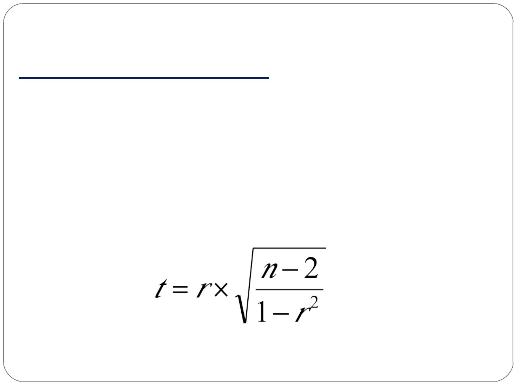
is small. The simplest formula for
computing the appropriate t value to test significance of a
correlation coefficient employs the t-distribution with df=n
-2

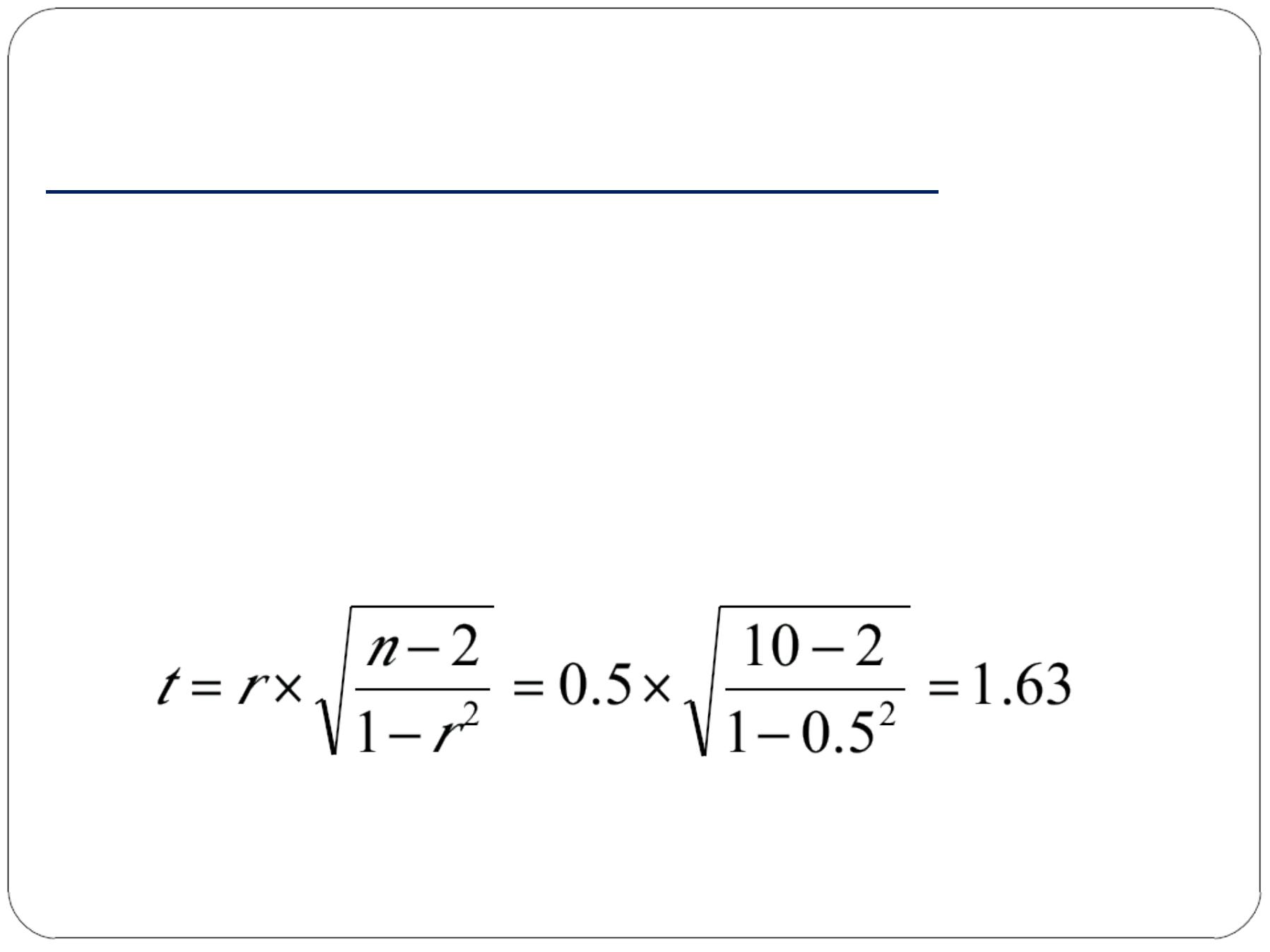
Testing significance of (r)-Example
Example: Suppose you observe that
r= 0.50
between literacy
rate and political stability in 10 nations. Is this relationship
"strong"? Is it significant statistically?
—
Since
r
r
is between 0.4 to 0.69, the linear correlation is
moderately strong “
c
c
l
l
i
i
n
n
i
i
c
c
a
a
l
l
l
l
y
y
s
s
i
i
g
g
n
n
i
i
f
f
i
i
c
c
a
a
n
n
t
t
”
!
For
d
d
f
f
=
=
n
n
-
-
2
2
=
=
1
1
0
0
-
-
2
2
=
=
8
8
and one-tailed test (unidirectional test, since
we want to see that >0 at =0.05), the critical value (decision
rule) of
t
t
1- =1-0.05=0 .95, df=8
= 1.86
.
—
We calculate the “
Test Statistic”
t
t
=
=
1
1
.
.
6
6
3
3
, which is
<
<
than the
c
c
r
r
i
i
t
t
i
i
c
c
a
a
l
l
t
t
of 1.86. So the null hypothesis of no relationship in the
population ( =0) cannot be rejected and we conclude that
there is no statistically significant linear correlation between
literacy and political stability.
Testing significance of (r)-comments
Note that a relationship can be strong and yet not
significant. Conversely, a relationship can be weak but
significant. The key factor is the size of the sample (n).
For large samples, it is easy to achieve significance, and
one must pay attention to the strength of the correlation
to determine if the relationship makes sense.

Example
-Systolic Blood
Pressure Readings (mmHg)
by two methods in 25
Patients with Essential
Hypertension
Patient No.
Method I
Method II
1
132
130
2
138
134
3
144
132
4
146
140
5
148
150
6
152
144
7
158
150
8
130
122
9
162
160
10
168
150
11
172
160
12
174
178
13
180
168
14
180
174
15
188
186
16
194
172
17
194
182
18
200
178
19
200
196
20
204
188
21
210
180
22
210
196
23
216
210
24
220
190
25
220
202
Method I
M
e
th
o
d
II
Systolic Blood pressure readings (mm Hg), 25 Patients with essential hypertension

Patient No.
Method I
Method II
X
2
Y
2
XY
1
132
130
17424
16900
17160
2
138
134
19044
17956
18492
3
144
132
20736
17424
19008
4
146
140
21316
19600
20440
5
148
150
21904
22500
22200
6
152
144
23104
20736
21888
7
158
150
24964
22500
23700
8
130
122
16900
14884
15860
9
162
160
26244
25600
25920
10
168
150
28224
22500
25200
11
172
160
29584
25600
27520
12
174
178
30276
31684
30972
13
180
168
32400
28224
30240
14
180
174
32400
30276
31320
15
188
186
35344
34596
34968
16
194
172
37636
29584
33368
17
194
182
37636
33124
35308
18
200
178
40000
31684
35600
19
200
196
40000
38416
39200
20
204
188
41616
35344
38352
21
210
180
44100
32400
37800
22
210
196
44100
38416
41160
23
216
210
46656
44100
45360
24
220
190
48400
36100
41800
25
220
202
48400
40804
44440
Total
4440
4172
808408
710952
757276
n ∑XY-( ∑X) ( ∑Y)
r =----- ---- ---- ---- ---- ---- ---- ---- ----- ---- -- (not for
memorization)
√[ n∑X
2
–(∑X)
2
] [ n ∑Y
2
–(∑Y)
2
]
(25)(757276) -(4440) (4172)
r =---------------------------------------------------------------
√[ (25)(808408) –(4440)
2
][ (25)(710952) –
(4172)
2
]
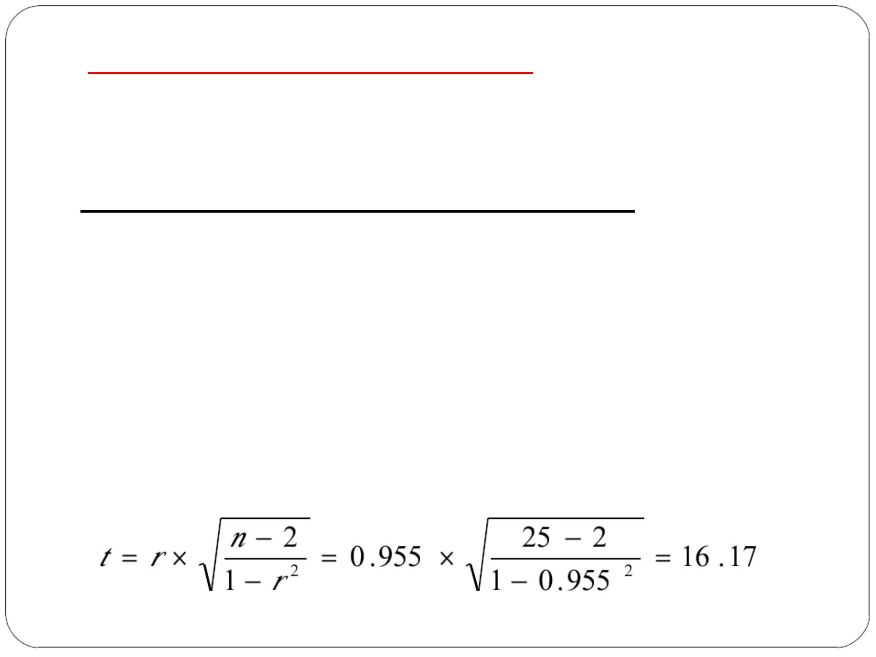
408220
=--------------= 0.955
427611.05
H
H
o
o
ρ
ρ
=
=
0
0
,
,
H
H
A
A
ρ
ρ
≠
≠
0
0

Critical value (decision rule)
t
1- =0.95, df=23
= 1.714
|Test statistic| > |Decision rule|
So we reject the H
o
in favor of H
A
, There is a statistically
significant very strong positive (direct) linear correlation
between the 2 methods of measuring blood pressure.

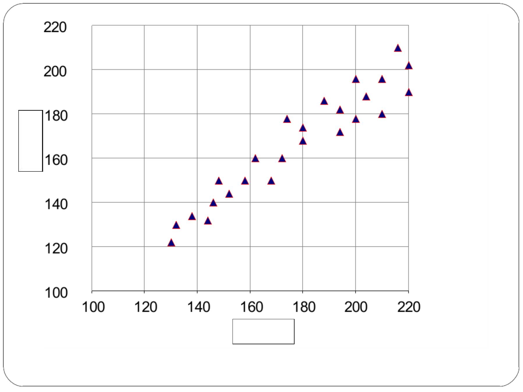
Scatter Diagram
—
The form of the relationship between two variables can be
presented visually in a Scatter Diagram which is a graphic
device used to visually summarize the relationship between
two variables
—
The X-axis is the horizontal axis and represents the
independent variable, while Y–
axis is the vertical axis and
represents the dependent variable. In correlation model one
need not know which is the dependent and independent
variable, while in regression model this distinction is crucial.
—
The closer the dots that represent pairs of observations for
study subjects to the regression line the stronger is the linear
correlation.
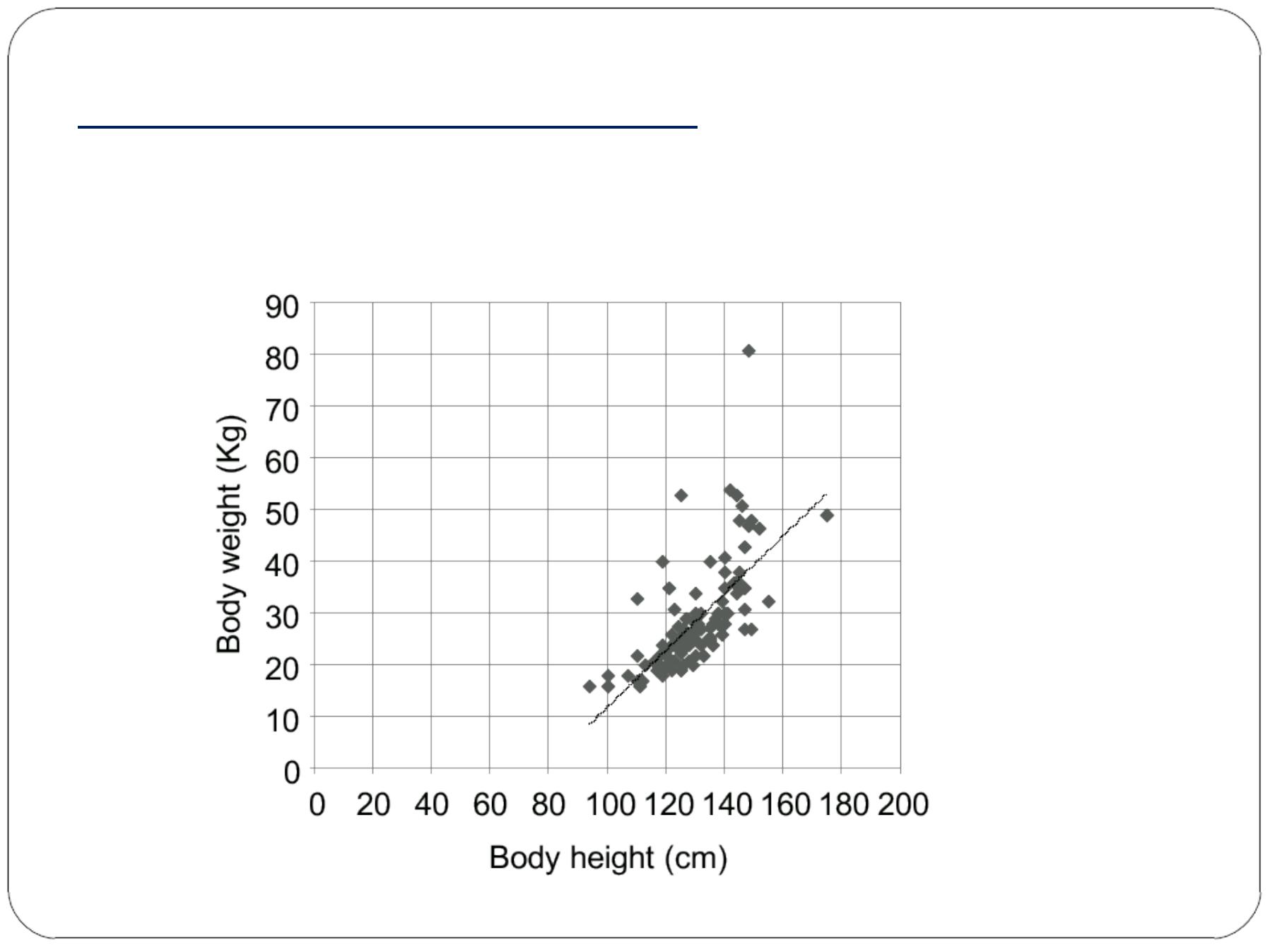
Scatter Diagram-example
Scatter diagram with fitted regression line (r=0.81)
There is a strong (r=0.81) positive linear correlation
between body weight and body height in children and
adolescents.
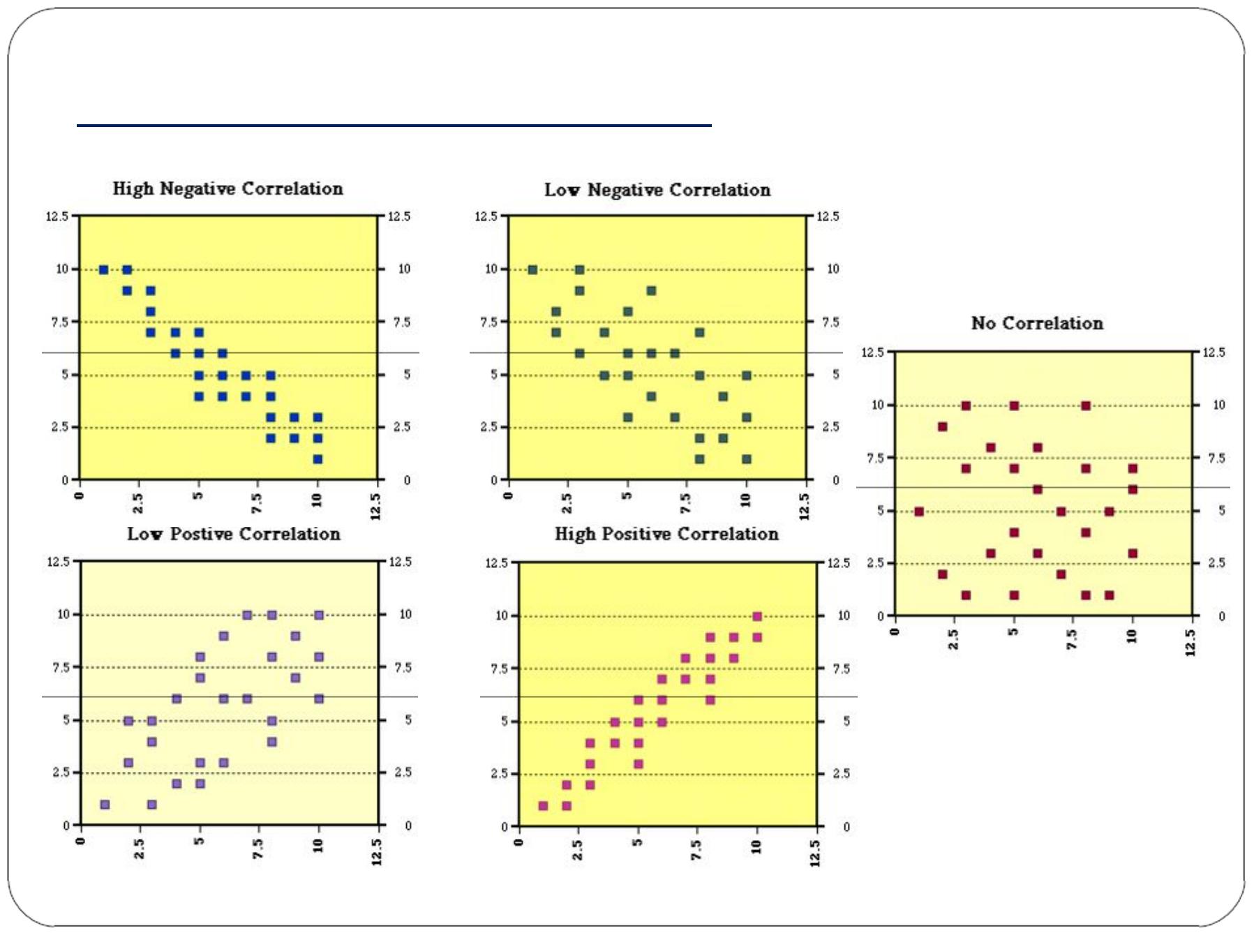
Scatter Diagram-examples

Simple Linear Regression
It is helpful in:
—
Ascertaining the probable form of the relationship
between variables.
—
Predict or estimate the value of one variable
corresponding to a given value of another variable.
—
Another way to quantify the strength of association
between 2 quantitative variables under the assumption
of normal distribution (
D
D
o
o
s
s
e
e
-
-
r
r
e
e
s
s
p
p
o
o
n
n
s
s
e
e
r
r
e
e
l
l
a
a
t
t
i
i
o
o
n
n
s
s
h
h
i
i
p
p
).
R
R
e
e
m
m
e
e
m
m
b
b
e
e
r
r
:
:
The independent variable (x) is pre-selected
and called non-random or mathematical variable. For each
value of x there is a set of normally distributed values of
Y.

Simple Linear Regression-2
The least square method is used to predict the regression line
that best represents the linear relationship between X and Yas
shown in the formula below:
Y
= a+ b
x
a= intercept (constant): the point where the line crosses the
vertical axis (i.e. amount of Ywhen X= 0)
b=slope (regression coefficient): amount by which Ychanges
for each unit change in X . If its value is negative, for each
unit increase in x the Yis expected to decrease by a mean
quantity of b. However if its value is positive, we expect that
Yincreases by a mean quantity of b for each unit increase in
x.
X=independent (explanatory) variable
Y=dependant (response) variable

Simple Linear Regression-3
1.
Use of regression model for prediction:
If we enter
a specific value of X in the regression equation one can
predict the value of Y.
2.
Use of regression model for assessing the effect
size
or strength of association between 2 quantitative
variables measured on interval/ ratio scale. The higher
the value of b (regression coefficient) the stronger is
the effect of x (independent, explanatory or exposure)
on the value of Y (dependent, response or outcome).
i.e. stronger dose-response linear relation.

Simple Linear Regression-3
3.
Power of prediction of the model:
The overall
prediction power of the model is measured by R
2
(
d
d
e
e
t
t
e
e
r
r
m
m
i
i
n
n
a
a
t
t
i
i
o
o
n
n
c
c
o
o
e
e
f
f
f
f
i
i
c
c
i
i
e
e
n
n
t
t
) which is equal to the
square value of r (linear correlation coefficient). It
measures the proportion of observed variation in the
response variable explained by the regression model.

Simple Linear Regression-4
—
The
least square method
is used to estimate the 2
points needed to draw the regression line. The
predicted value for Y which lies on the regression line,
based on the specific value of X should give the least
possible error from the actual values of Y associated
with that X value.
—
The calculated regression coefficient (beta or slope) is
also tested for statistical significance by t-test against
the null hypothesis of
beta=0
at the population level.
—
The overall regression equation is tested for statistical
significance
by
A
A
N
N
O
O
V
V
A
A
.
The
model should
be
statistically significant before we are able to generalize
the results to reference population.

Example:
To evaluate the performance of a new test on 11
patients an e xperiment was done with paired measurements of
scores obtained on the new te st and the standardize d test. The
results are shown below
Patient No.
Score on New Test (X)
Score on standardized Test (Y)
1
50
61
2
55
61
3
60
59
4
65
71
5
70
80
6
75
76
7
80
90
8
85
106
9
90
98
10
95
100
11
100
114

Patient
No.
Score on
New
Test (X)
Score on
standardized Test
(Y)
X
2
Y
2
XY
1
50
61
2500
3721
3050
2
55
61
3025
3721
3355
3
60
59
3600
3481
3540
4
65
71
4225
5041
4615
5
70
80
4900
6400
5600
6
75
76
5625
5776
5700
7
80
90
6400
8100
7200
8
85
106
7225
11236
9010
9
90
98
8100
9604
8820
10
95
100
9025
10000
9500
11
100
114
10000
12996
11400
825
916
64625
80076
71790

n∑XY –
[ (∑X) (∑Y)]
b =------------------------- (not for memorization)
n∑X
2
–(∑X)
2
[ (11)(71790)] –
[ (825) (916)]
b =------------------------------------------= 1.124
[(11)(64625)] –(825)
2
∑Y–b ∑X
916 –[ 1.1236 (825)]
a =------------------
= ----------------------------- = - 0.997
n
11
Y= a + bX
Y=- 0.997 + 1.124 X
For each one score increase in X the value of Yis expected to
increase by a mean of 1.124 score.
Scores on new test
S
c
o
re
s
o
n
s
ta
n
d
a
rd
iz
e
d
te
s
t