
Association between two
categorical variables
Dr. Ahmed Samir Al-Naaimi
MBChB, MSc epid, PhD
Assistant Professor / Department of Community Medicine
Baghdad College of Medicine

Learning objectives
1.
The student will analyze the relationship between
two categorical variables with two or more
categories.
2.
Apply the Chi-square test for hypothesis testing.
3.
Understand the concept of observed and expected
frequencies.
4.
Explore the link between Chi-square test and
multiplication rule used for joint probability under
the assumption of independence between 2
classification criteria.

Learning objectives
5.
Relate the magnitude of difference between
observed and expected frequency to resulting test
statistic
and
the
conclusion
of
statistical
significance.
6.
Evaluate the link between Z test and Chi-square test
in the special condition of 2 x 2 contingency table.
7.
List the conditions for a valid Chi-square test.

Introduction
The table shows the distribution of individuals according
to 3 categories of Socioeconomic Index Level (SEIL).
SEIL
N
%
Low
50
25
Average
110
55
High
40
20
Total
200
100

Introduction
In the same sample the location of residence was also
classified into 3 sectors: south, center and north.
N
%
South
44
22
Center
96
48
North
60
30
Total
200
100

Introduction
When we examine the relationship between two
categorical variables, tabulated one against other.
This is a two way table or cross-tabulation.
Location
SEIL
South
Center
North
Total
Low
33
7
10
50
Average
9
81
20
110
High
2
8
30
40
Total
44
96
60
200

Interpretation of a two by two table
There is an association between two categorical
variables, if the distribution of a variable varies
according to the value of the other.
The question we are interested in “Does the Socio-
economic Index level (SEIL) varies by place of
residence?
To answer this question we need to assess a cross-
tabulation and calculate relative frequencies
(percentages).

Interpretation of a two by two table
To answer the question of interest, what should we consider
the relative frequencies of column or row totals?
SEIL
South
n %
Center
n %
North
n %
Low
33 75
7 7.3
10 16.7
Average
9 20.5
81 84.4
20 33.3
High
2 4.5
8 8.3
30 50
Total
44 100.0
96 100.0
60 100.0
Place of residence

Interpretation of a two by two table
If the distribution of SEIL is the same in each place of
residence, the percentage of columns would be the
same for each place of residence. It appears that the
percentage of low SEIL differ between sites of
residency, but the data are subject to sampling errors, so
we need to assess whether these differences in the
proportions of the sample reflect differences in
populations.
To do this, we need a hypothesis test.
Expected frequencies
If the null hypothesis is true
, there is no association
between SEIL and area of residence, the percentages for
each level of SEIL in each area, should be the same as
the column of percentages in the total column. Or one
can state the hypothesis as
“the 2 methods of
classification for people: SEIL and place of residence
are independent”

SEIL
South
n %
Center
n %
North
n %
Total
n %
Low
33 75 7 7.3 10 16.7 50 25
Regular
9 20.5 81 84.4 20 33.3 110 55
High
2 4.5 8 8.3 30 50 40 20
Total
44 100.0 96 100.0 60 100.0 200 100.0
Place of residence
Interpretation of a two ways table
Also, we should expect than 25% of people in the South
have low SEIL. so the frequency (count) of people in
South sector of residence with low SEIL is 0.25 x 44 = 11.

Expected frequencies
If there are no differences in the distribution of SEIL
by places of residence, we should expect that the
relative frequency of people with low SEIL is the
same in each place of residence.
Note that the expected frequencies do not have to be
integers.
Using the totals of columns and rows, we can
calculate the expected frequency (count) in each cell.
E = (row total x column total) / grand total
Expected frequencies
Under the null hypothesis of independence for 2 events,
the joint probability is equal to the product of the
probability of each event.
P (Low SEIL) = 50/200
P (South) = 44/200
P (Low SEIL and South) =
50/200 x 44/200
The frequency expected in (Low SEIL and South) is
equal to the P (Low SEIL and South) multiplied by total
sample size of 200.
Expected frequency (E) = 50/200 x 44/200 x 200
E = (row total x column total) / grand total
Location
SEIL
South
Center
North
Total
Low
33
50
Average
110
High
40
Total
44
96
60
200

Chi-square test
Expected frequencies are those that we should expect
if the null hypothesis were true.
To test the null hypothesis, we must compare the
expected frequencies with observed frequencies, using
the following formula.
E
E
O
2
2

Chi-Square test
From the formula we can see that:
If there is a large or significant difference between the
observed and expected values, the calculated (test
statistic)
2
will be large, while if there is a small (or
statistically insignificant) difference between the
observed and expected values, the resulting
2
will be
small also.

Chi-Square test
If the calculated (test statistic)
2
is large, then the
sample data provides enough evidence to reject the
null hypothesis (H
o
) because the observed values are
not what we expect under the null hypothesis.
If the calculated (test statistic)
2
is small in
magnitude, then the sample data agrees with (accepts)
the null hypothesis (H
o
), which states that the
observed values are similar to or not significantly
different from those expected under the null
hypothesis of independence.
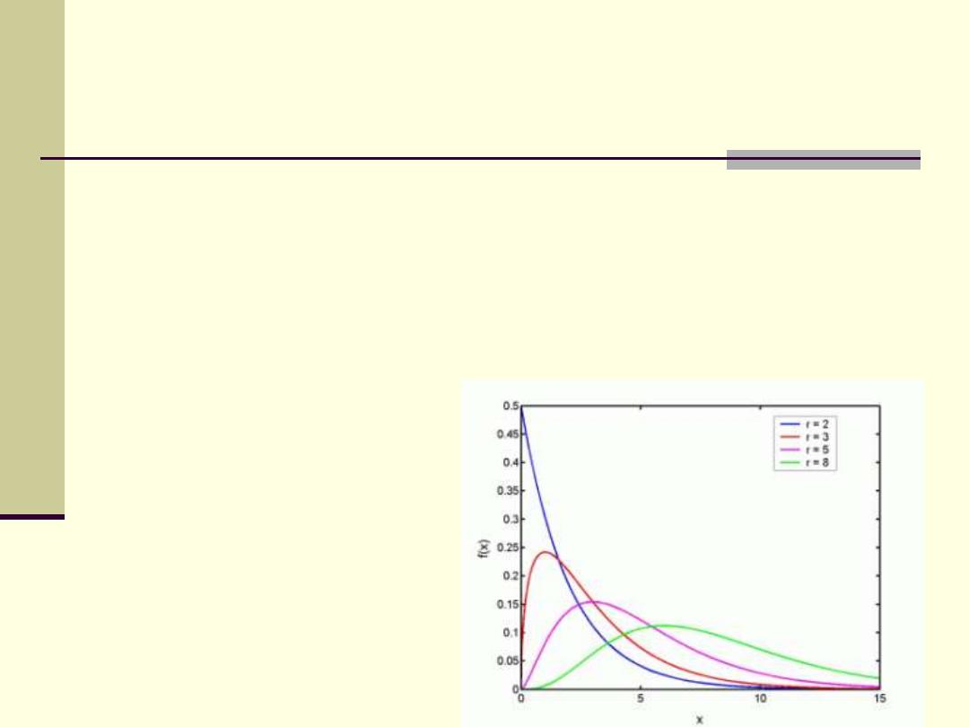
Chi-Square distribution
The values of test statistic in Chi-square distribution is
between zero and + ∞. No negative values are present
since they are squared values.
The Chi-square distribution has one tail only (positively
skewed distribution).
The higher the df the
more flattened is the
curve.
Hypothesis testing is
always one tailed

Chi-Square test
The X
2
distribution is obtained from the sum of the
squares of many standard Normal variables. The number
of independent variables commonly used in this sum is
the “degrees of freedom”, df = (r-1) x (c-1), where r is
the count of rows in the table and c is the count of
columns.
The tabulated X
2
for 2x2 table with df=1 and alpha error
= 0.05 is equal to (Z
1-alpha/2
)
2
= (1.96)
2
= 3.84.
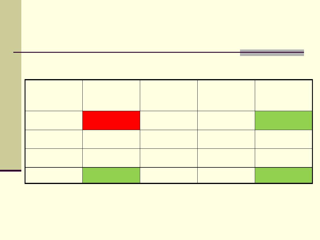
Chi-Square test
SEIL
South
O E
Center
O E
North
O E
Total
n
Low
33 11 7 24 10 15
50
Regular
9 24.2 81 52.8 20 33
110
High
2 8.8 8 19.2 30 12
40
Total
44 44
96 96 60 60 200
Place of residence
Expected frequency = row total x column total /grand total.
Example: the expected frequency in the first cell of the table (the left
upper) = (50 x 44) / 200 = 11, while the observed frequency is 33.

Chi-Square test
SEIL
Place of
residence Observed
Expected
O - E
(O-E)
2
(O-E)
2
/E
Low
South
33
11
22
484
44
Low
Center
9
24
- 15
225
9.38
Low
North
2
15
- 13
169
11.27
Regular South
7
24.2
-17.2
295.8
12.2
Regular Center
81
52.8
28.2
795.2
15.1
Regular North
8
33
- 25
625
18.9
High
South
10
8.8
1.2
1.44
0.2
High
Center
20
19.2
0.8
0.64
0.03
High
North
30
12
18
324
27
Total
138.1

Steps for hypothesis testing
1. State the statistical hypothesis
H
o
: There is no association between SEIL and
residence location
H
A
: There is an association
2. Fill in the observed frequencies for contingency table.
3. Calculate expected frequencies.
4. Calculate the test statistic (Chi-square)
5. Calculate the degrees of freedom (df) = (r-1) x (c-1)
= (3-1) x (3-1) = 2 x 2 = 4
6. Get the tabulated
2
(decision rule) for the specified df.

Steps for hypothesis testing
6. The tabulated X
2
(decision rule) for df=4 is 9.5
7. Compare the test statistic (calculated X
2
) and decision
rule. Since 138.1 is > 9.5, then reject the H
o
in favor of
H
A
.
8. Conclusion: there is a statistically significant
association between SEIL and residence location.

Chi-Square test in 2 x 2 tables
When both variables are binary (dichotomous), the
cross-tabulation table becomes a 2 x 2.
The
2
test can be applied in the same way as for a
larger number of categories table.
This special condition for
2
is very common in medical
literature. It will give the same result as that of Z test
used for the difference between 2 proportions studied
earlier in the biostatistics module. Remember that the
decision rule for
2
at df=1 is 3.841 which is the square
value of Z at alpha 0.05 = 1.96.

Example (2 x 2 table)
There was a study of the bacteriological efficacy of
clarithromycin Vs penicillin, in acute pharyngo-tonsillitis
in children by Streptococcus Beta Haemolytic Group A.
The results are shown below
Drug
Cure
Not cure
Total
Clarithromycin
91
9
100
Penicillin
82
18
100
Total
173
27
200

Example (2 x 2) table
Statistical hypothesis
H
o
: There is no association between type of treatment and cure.
While in case of Z test we would say “There is no difference in
bacteriological efficacy (response rate) between the two
treatments, against Streptococcus Beta Hemolytic Group A.
H
A
: There is an association between type of treatment and patient’s
response to treatment.
Drug
Cure
O E
Not cure
O E
Total
Clarithromycin 91 86.5 9 13.5
100
Penicillin
82 86.5 18 13.5
100
Total
173
27
200
Drug
Effect
Observed Expected O - E
(O-E)
2
(O-E)
2
/E
Clarithromycin Cure
91
86.5
4.5
20.25
0.234
Clarithromycin Not cure
9
13.5
- 4.5
20.25
1.5
Penicillin
Cure
82
86.5
- 4.5
20.25
0.234
Penicillin
Not cure
18
13.5
4.5
20.25
1.5
Total
3.47
df = (r-1) x (c-1) = (2-1) x (2-1) = 1 x 1 = 1
Calculate expected frequencies
Calculate the test statistic (
2
) for each cell in the table
and its sum = 3.47
Get the decision rule
2
at df=1 which is 3.841
Example (2 x 2) table

Compare the test statistic (3.47) and decision rule (3.841),
since the test statistic is larger, we accept the H
o
.
Conclusion: There is no statistically significant
association between the type of treatment and
the patients response to treatment
Try to solve this example by Z test and
compare the results obtained by both
methods.
Example (2 x 2) table
A quick formula for 2 x 2 tables
2
can be calculated without the need for expected
frequencies in the special case of 2 x 2 table. Use the
observed frequencies in a table and marginal totals. If
we labeled the cells and marginal totals as follow:
Exposure
Result
Yes
Result
No
Total
Yes
a
b
a + b
No
c
d
c + d
Total
a + c
b + d
N
2
=[(ad
– bc)
2
x N ]/[(a+b) (c+d) (a+c) (b+d)]

Validity of Chi-Square tests
Chi square tests are based on the assumption that the
test statistic follows approximately the
2
distribution.
This is reasonable for large samples but for the small
one we should use the following guidelines:
a) For 2 x 2 tables
If the total sample size is> 40, then
2
can be used.
If n is between 20 and 40, and the smallest expected
value is > 5,
2
can be used. Otherwise, use the
Fisher exact significance test.
b) For r x c tables:
The
2
test is valid if not more
than 20% of expected values is less than 5 and none
is less than 1.