
HYPOTHESIS TESTING
Asst Prof Dr. Ahmed Sameer Alnuaimi

Learning objectives
1.
Define research hypothesis.
2.
Define statistical hypotheses.
3.
State the purpose of hypothesis testing.
4.
Value the difference between parametric and non-
parametric statistical hypotheses.
5.
Define “Test Statistics”.
6.
Learn the formula for calculating “Test Statistic” in case of
single proportion, difference between 2 proportions, single
mean (under the condition of known and unknown
population variance), difference between 2 means (under
the condition of known and unknown population variance,
with assumption of equal and unequal population
variances)

Learning objectives
7.
Define type-I and type-II errors in hypothesis testing.
8.
Define P value.
9.
Define rejection region and acceptance region.
10.
Master the 8 steps of hypothesis testing procedure.
11.
Master the interpretation of hypothesis testing procedure.
Research Hypothesis
1.
It is the assumption that motivate the research. It
is usually the result of long observation by the
researcher. It is stated in a direct type of
language. For example: “Is there a difference in
school achievement between males and females”.
2.
This type of hypothesis lead directly to the second
type of hypothesis, called Statistical Hypothesis.
Hypothesis Testing
Purpose
The purpose of hypothesis testing is to help the researcher
or administrator in reaching a decision concerning a
population by examining a sample from that population.
Definition of Statistical Hypothesis
It is a statement about one or more population. Usually
concerned with the parameter of the population about
which the statement is made (parametric hypothesis is
used with tests based on normally distributed data).
An exception is noticed with non-parametric (distribution
free) tests (like Chi-square test and Mann-Whitney test),
in which no parameters are mentioned in the hypothesis
statement
Statistical Hypothesis
It is stated in a way that can be evaluated by
appropriate statistical techniques. It is composed of
two types:
1.
Null hypothesis( Ho):
It is the particular
hypothesis under test. It is the hypothesis of “no
difference or no association”.
2.
Alternative hypothesis (HA):
which disagrees
with the null hypothesis (and usually agrees with
the research hypothesis).
Test Statistic
It is a mathematical expression, which provides a
basis for testing a statistical hypothesis .
The result of this test will determine whether we
will accept the Null hypothesis and as a results
reject the
H
A
(i.e. the researcher will be
disappointed, because his theory does not hold
and can not be generalized from the sample to
the population). Or we reject the null hypothesis
and so the
H
A
will be accepted (i.e. the
researcher will happily generalize the findings of
his sample to the reference population).

Errors
There are two possible errors with hypothesis testing
(false conclusions being made), since they are based
on the concept of probability:
Type 1 error (alpha error):
Rejection of the null hypothesis when it is true (i.e.
reporting an important difference, when in fact at the
level of population there is non. The difference
observed in the sample was in fact a chance finding.
It is presented by alpha, which is the level of
significance, often the 5% and to a lesser extent the
0.1% (
α=0.05, and 0.001) levels are chosen.

Alpha error
It is the level of chance tolerated by the researcher as
an alternative explanation for the results of the
sample.
It is of small magnitude (5% or 1/1000), but it needs to
be remembered and taken into account when the
stakes are high, like for example in case of dangerous
disease or complications. (Thalidomide disaster is an
example).

Beta Error
Type I1 error (Beta error):
Accepting the null hypothesis when it is false. i.e.
There is a real effect or difference, but the researcher
is unable to accept the alternative hypothesis. It
denotes failure to detect a real effect or difference.
The power of study to detect an effect is measured by
“one minus Beta error”.
This error is not evaluated by the type of statistical
methods tough in biostatistics module. It needs more
advanced statistical tools. Usually studied in relation
to sample size estimation.
A larger sample size will result in lower type-II error
and higher study power.
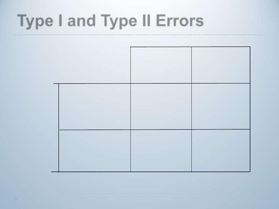
Type I and Type II Errors
True State of Nature
We decide to
reject the
null hypothesis
We fail to
reject the
null hypothesis
The null
hypothesis is
true
The null
hypothesis is
false
Type I error
(rejecting a true
null hypothesis)
Type II error
(rejecting a false
null hypothesis)
Correct
decision
Correct
decision
De
cis
io
n
P-value
It is the smallest value of
α
(alpha) for which the
Ho
can be rejected.
It gives a more precise statement about probability of
rejection of
Ho
when it is true than the alpha level,
so instead of saying the test statistic is significant or
not , we will mention the exact probability of rejecting
the
Ho
when it is true.
It measures the role in chance in finding an effect or
difference in the sample studied.
Steps in conducting hypothesis
testing
Hypothesis testing can be presented as 8 steps process:
1. Data :
The nature of the data whether it consists of counts, or
measurement will determine the test statistic to be
used (z test, t-test, Chi-square test, ANOVA).
2. State the 2 Statistical Hypotheses :
Null Hypothesis (
H
o
)
and the alternative hypothesis(
H
A
).
If
we accept the
H
o
we will say that the data to be tested
does not provide sufficient evidence, based on the
current sample to cause rejection.
If
H
o
is rejected we say that the data are not compatible
with
H
o
and support the alternative hypothesis (
H
A
).
Steps in conducting hypothesis
testing
3
. Identify the “Test Statistic” to be used:
Use the data of
the sample to reach to a decision to reject or
to accept the null hypothesis. The general
formula for a test statistic is:
Statistic - Hypothesized
parameter
Test Statistic = --------------------------------------------
--
Standard Error (SE) of the
statistic
4. Identify the distribution of test statistic:
(refer to step 1)
5. Identify
“Decision Rule” from statistical tables:
It will tell
us to reject the null hypothesis if the test statistic falls in
the rejection area, and to accept it if it falls in the
acceptance region

Decision Rule
The critical values (tabulated value) that discriminate
between acceptance and rejection regions
depending on alpha level of significance.
If the value of the test statistic falls in the rejection
region area, it is considered statistically significant. If
it falls in the acceptance area it is considered not
statistically significant
Whenever we reject a null hypothesis , there is
always a possibility of type 1 error (rejection of
H
o
when it is true). This is why we should decrease this
error to the least possible.

The value of the test statistic that separate the
rejection region from the acceptance region
Acceptance region:
A set of values of the test
statistic leading to acceptance of
the null hypothesis (values of the
test statistic not included in the
critical region)
Rejection region:
A set of values of the test statistic
leading to rejection of the null
hypothesis
Critical value
6. Computing Test Statistic:
7. Statistical decision:
It consists of rejecting or
accepting (not rejecting) the
H
o
. It is rejected if the
computed value of the test statistic falls in the
rejection area
(its absolute value ≥ absolute value
of decision rule),
and it is not rejected if computed
value of the test statistic falls in the acceptance
region
(its absolute value < absolute value of
decision rule).
8. Conclusion:
If
H
o
is rejected , we conclude that
H
A
is true, while If
H
o
is not rejected we conclude that
H
A
may be true.
Steps-continued

Two sided test :
If the rejection area is divided
into the two tails the test is called
two-sided test. (this is the usual
condition)
One sided test:
If the rejection region is only in
one tail it is called one-sided test.
The decision will depend on the nature of the
research question being asked by the researcher.
Note:
If we can reject the Ho on a two sided test
(statistically significant finding) it will also be
significant on a one sided test. The reverse is not
true.
1. Single population mean , known population
variance
_
X - µ
Z=-------------
σ /√ n
2. Single population mean with unknown population
variance
_
X - µ
t =-------------
S /√ n
Computing test statistic
3. Difference between two populations mean with
known variances
_ _
(X
1
–X
2
)
– (µ
1
-µ
2
)
Z=-------------------------------
√ σ
2
1
/n
1
+
σ
2
2
/n
2
4. Difference between two populations mean with
unknown and unequal variances
_ _
(X
1
–X
2
)
– (µ
1
-µ
2
)
t =-------------------------------
√ s
2
1
/n
1
+ s
2
2
/n
2
Computing test statistic-continued
5. Difference between two populations mean with
unknown but assumed equal variances
_ _
(X
1
–X
2
)
– (µ
1
-µ
2
)
t =-------------------------------
S
p
√ 1 /n
1
+ 1
/n
2
6. Mean difference (paired t-test)
_
d -µ
d
t =-------------
S
d
/√ n
Computing test statistic-continued

7. Single population proportion
P
– P
Z = -------------
√P(1-P)/n
8. Difference between two population proportions
(P
1
-P
2
)
–(P
1
-P
2
)
Z=-----------------------------------------
√P
1
(1-P
1
)/n
1
+ P
2
(1-P
2
)/n
2

Example-1
A certain breed of rats shows a mean weight gain of
65 gm, during the first 3 months of life. 16 of these rats
were fed a new diet from birth until age of 3 months.
The mean was 60.75 gm. If the population variance is
10 gm , is there a reason to believe at the 5% level of
significance that the new diet causes a change in the
average amount of weight gained

H
o
: µ =65
H
A
: µ
≠ 65
Z
1-
α/2=1-(0.05/2)=0.975
α=0.05 Z=1.96 (Decision rule
or critical
value)
_
x -µ 60.75-65
Z=---------- = ----------- = -5.38
σ /√n √10/ √16
Sine the calculated value falls in the rejection region
(its
absolute value ≥ absolute value of decision rule or 5.38 ≥1.96)
,
we reject the H
o
, and accept the H
A.
The new diet causes
a statistically significant change in the average amount of
weight gained.
Solution

In the previous example , if the population variance
is unknown, and the sample S (standard deviation
is 3.84
t
1-
α/2
= 2.13
df =n-1
_
X -µ 60.75-65
t =-------------=------------= - 4.13
s
/√n 3.84/ √16
Sine the calculated values falls in the rejection
region (its absolute value ≥ absolute value of
decision rule or 4.13
≥2.13), we reject the
H
o
, and
accept the
H
A
Example-2

In a study two types of dental cements were used to hold
a crown on tooth cast. The amount of force in foot
pounds required to pull each cemented crown from the
cast was reported :
_
X n
σ
-----------------------------------------------------------
Cement 1: 45 50 4.1
Cement 2: 42 50 3.4
Test the hypothesis that µ
1
= µ
2
at
α=0.05.
2. If
σ
1
and
σ
2
are unknown but assumed to be equal test
the same hypothesis if : S
1
=6.2 S
2
= 5.2.
3. If
σ
1
and
σ
2
are unknown and unequal test the same
hypothesis
Example-3

In a dental clinic it is hypothesized that 90% of all 4-
years old children give no evidence of dental caries. In
a study of 100 children 82 gave no such evidence ,
would you accept the quoted value of the 90% ? Use
α=0.05
Example-4

Two communities were sampled to learn about their
attitudes towards “organ donation after death” prior to
campaigns being launched. The results showing
favorable attitude towards the concept of after death
organ donation were :
n
1
= 110 n
2
= 75
˜ ˜
P
1
=0.52 P
2
=0.55
Does the two communities have equal proportions of
favorable attitude.
Example-4