First stage – College of Medicine – University of Mosul\ Nineveh
Computer-Lecture 9 / 2015-2016
maha al ani
1
9. Filtering Cells
Filtering or temporarily hiding data in a spreadsheet very easy. This allows you to
focus on specific spreadsheet entries
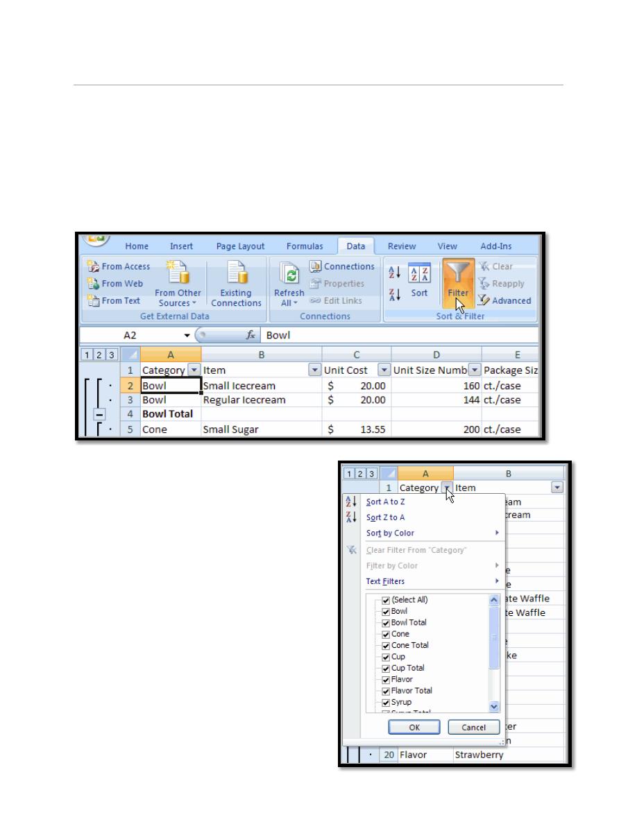
9.1. To Filter Data:
Click the Filter command on the Data tab. Drop-down arrows will appear besides
each column heading.
Click the drop-down arrow next to the
heading you would like to filter.
First stage – College of Medicine – University of Mosul\ Nineveh
Computer-Lecture 9 / 2015-2016
maha al ani
2
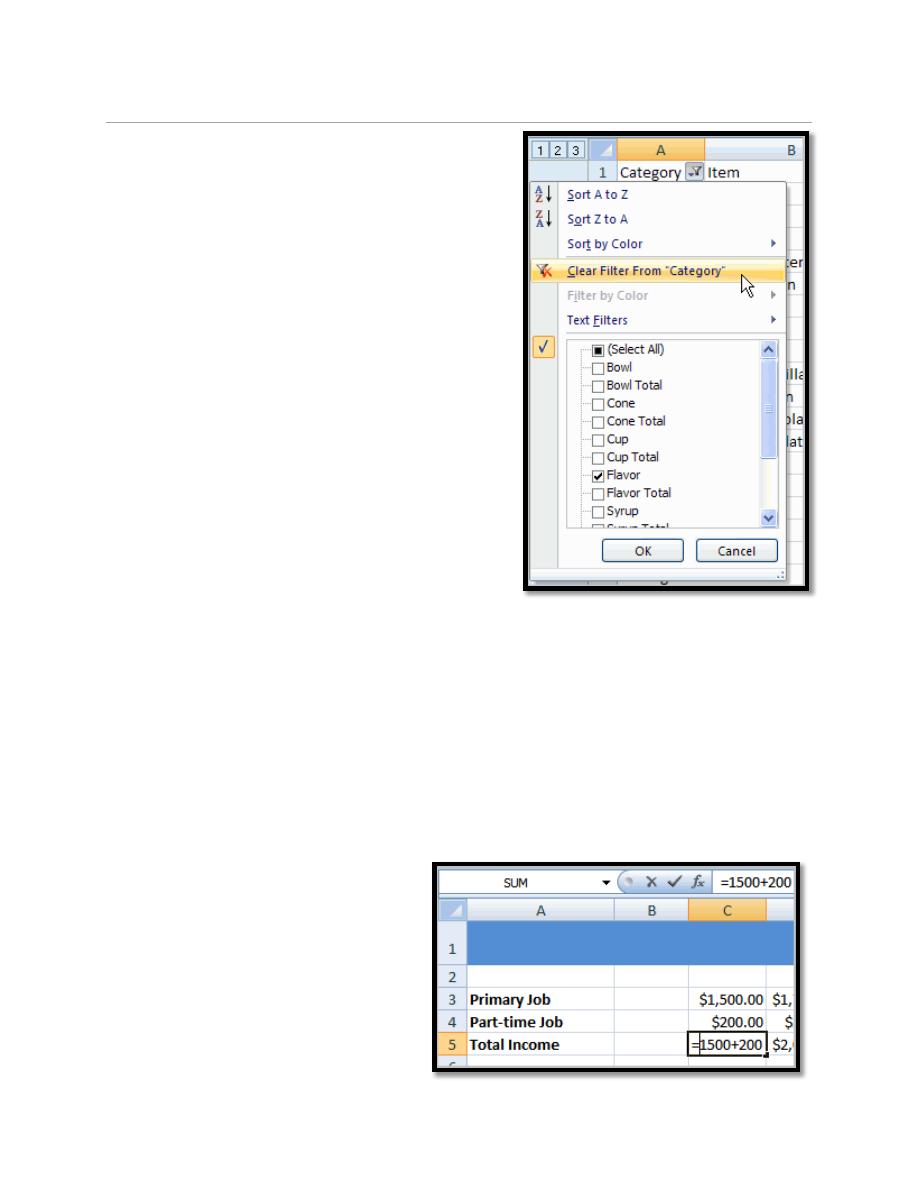
9.2. To Clear One Filter:
a. Select one of the drop-down arrows next to a
filtered column.
b. Choose Clear Filter From...
c. To remove all filters, click the Filter
command.
10. Simple Formulas
10.1. To Create a Simple Formula that Adds Two Numbers:
a. Click the cell where the formula will be defined (C5, for example).
b. Type the equal sign (=) to let Excel know a formula is being defined.
c. Type the first number to be added (e.g., 1500).
d. Type the addition sign (+) to let Excel know that an add operation is to be
performed.
e. Type the second number to be added (e.g., 200).
f. Press Enter or click the Enter button on the Formula bar to complete the
formula.
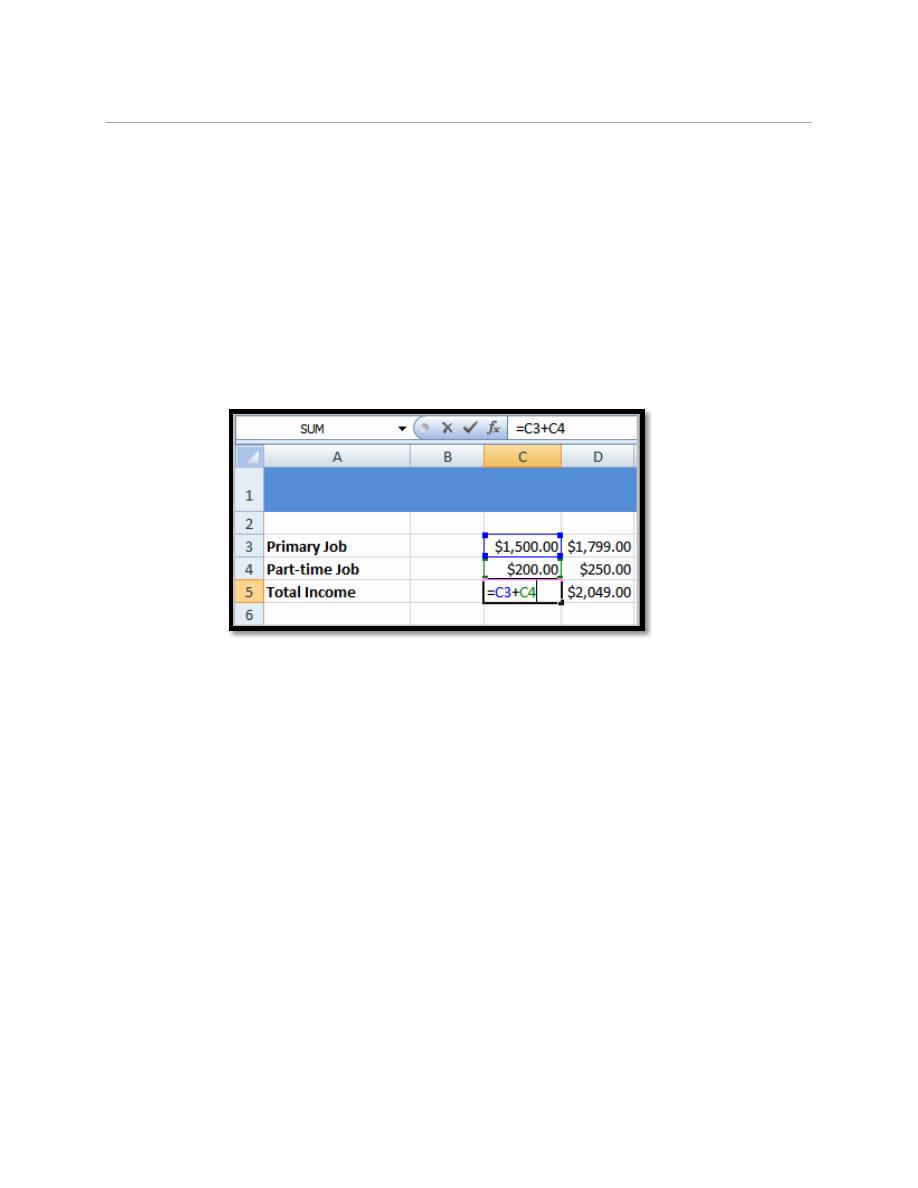
10.2. To Create a Simple Formula
that Adds the Contents of Two
Cells:
First stage – College of Medicine – University of Mosul\ Nineveh
Computer-Lecture 9 / 2015-2016
maha al ani
3
a. Click the cell where the answer will appear (C5, for example).
b. Type the equal sign (=) to let Excel know a formula is being defined.
c. Type the cell number that contains the first number to be added (C3, for
example).
d. Type the addition sign (+) to let Excel know that an add operation is to be
performed.
e. Type the cell address that contains the second number to be added (C4, for
example).
f. Press Enter or click the Enter button on the Formula bar to complete the
formula.
11. Basic Functions
The Parts of a Function:
Each function has a specific order, called syntax, which must be strictly followed
for the function to work correctly.
11.1. Syntax Order:
a. All functions begin with the = sign.
b. After the = sign define the function name (e.g., Sum).
c. Then there will be an argument. An argument is the cell range or cell references
that are enclosed by parentheses. If there is more than one argument, separate each
by a comma.
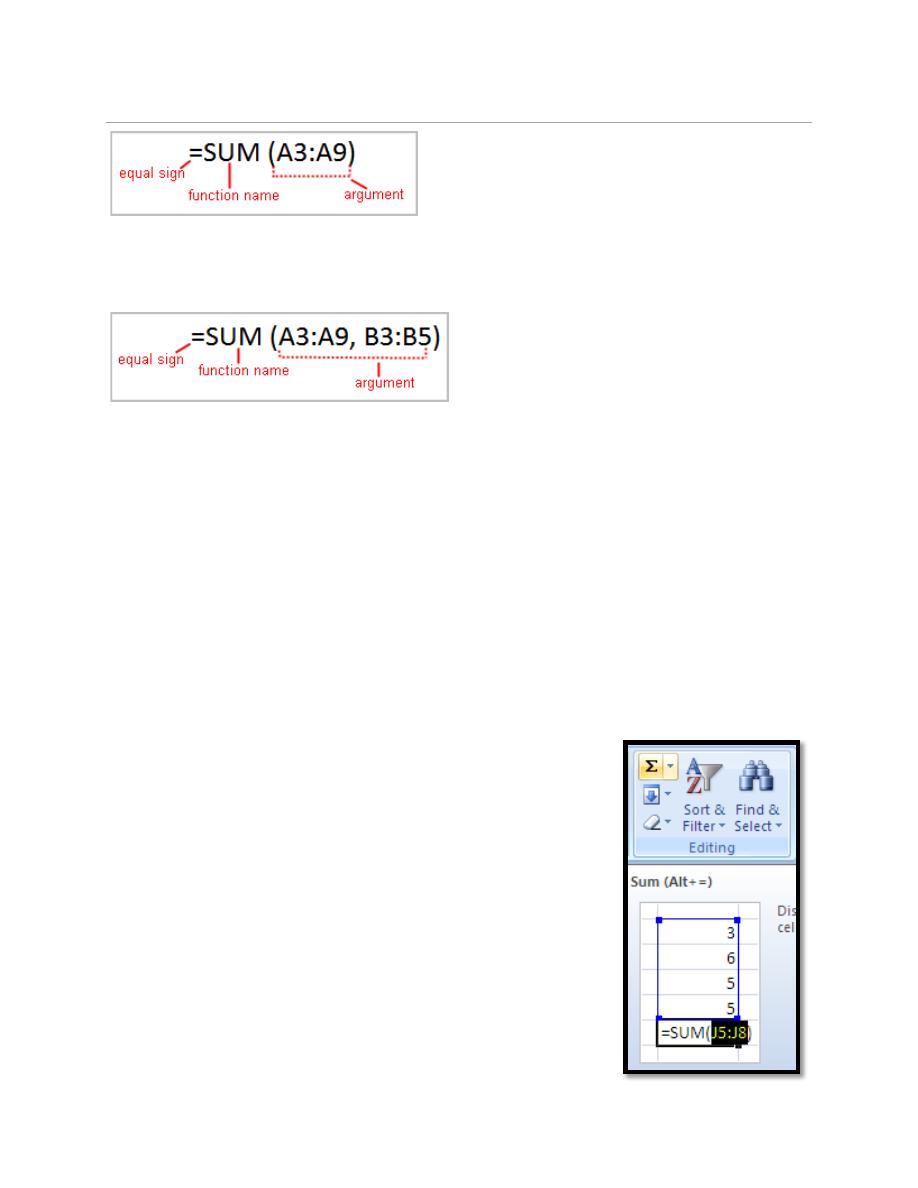
An example of a function with one argument that adds a range of cells, A3 through
A9:
First stage – College of Medicine – University of Mosul\ Nineveh
Computer-Lecture 9 / 2015-2016
maha al ani
4
An example of a function with more than one argument that calculates the sum of
two cell ranges:
11.2. Excel's Different Functions:
There are many different functions in Excel 2007. Some of the more common
functions include:
a. Statistical Functions:
(1) SUM - summation adds a range of cells together.
(2) AVERAGE - average calculates the average of a range of cells.
(3) COUNT - counts the number of chosen data in a range of cells.
(4) MAX - identifies the largest number in a range of cells.
(5) MIN - identifies the smallest number in a range of cells.
b. Date and Time functions.
Excel has mathematical functions for you to use.
o Total
Click on the Cell that displays a total.
In Home tab, click on the sum function icon, in the
Editing group.
Highlight the cells included in the total and hit Enter
key.
First stage – College of Medicine – University of Mosul\ Nineveh
Computer-Lecture 9 / 2015-2016
maha al ani
5
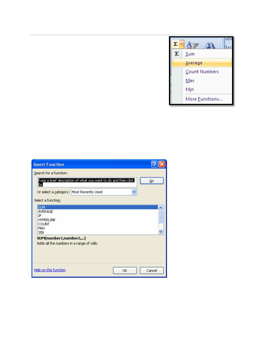
o Average
Click on the cell that displays an average.
In Home tab, click on the little down arrow in the
sum function icon and select Average.
Highlight the cells included in the average and hit
Enter key.
11.3. To Calculate the Sum of Two Arguments:
a. Select the cell where you want the function to appear. In this example, G44.
b. Click the Insert Function command on the Formulas tab. A dialog box appears.
c. SUM is selected by default.
d. Click OK and the Function Arguments dialog box appears so that you can
enter the range of cells for the function.

First stage – College of Medicine – University of Mosul\ Nineveh
Computer-Lecture 9 / 2015-2016
maha al ani
6
e. Insert the cursor in the Number 1 field.
f. In the spreadsheet, select the first range of cells. In this example, G21 through
G26. The argument appears in the Number 1 field.
g. To select the cells, left-click cell G21 and drag the cursor to G26, and then
release the mouse button.
h. Insert the cursor in the Number 2 field.
i. Click OK in the dialog box and the sum of the two ranges is calculated
Copy a Formula
You may copy the same formula onto a series of cells. By Drag the bottom right
corner of the cell to expand to the next cells.
.