THE SAMPLING DISTRIBUTION
DEFINITIONThe sampling distribution is a distribution of a sample statistic. While the concept of a distribution of a set of numbers is intuitive for most students, the concept of a distribution of a set of statistics is not. Therefore, distributions will be reviewed before the sampling distribution is discussed.
THE SAMPLE DISTRIBUTION
The sample distribution is the distribution resulting from the collection of actual data. A major characteristic of a sample is that it contains a finite (countable) number of scores, the number of scores represented by the letter N. For example, suppose that the following data were collected:
32
35
42
33
36
38
37
33
38
36
35
34
37
40
38
36
35
31
37
36
33
36
39
40
33
30
35
37
39
32
39
37
35
36
39
33
31
40
37
34
34
37
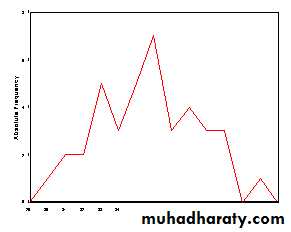
These numbers constitute a sample distribution. Using the procedures discussed in the chapter on frequency distributions, the following relative frequency polygon can be constructed to picture this data:
In addition to the frequency distribution, the sample distribution can be described with numbers, called statistics. Examples of statistics are the mean, median, mode, standard deviation, range, and correlation coefficient, among others.
THE SAMPLING DISTRIBUTION
Note the "-ING" on the end of SAMPLE. It looks and sounds similar to the SAMPLE DISTRIBUTION, but, in reality the concept is much closer to a population model.The sampling distribution is a distribution of a sample statistic. It is a model of a distribution of scores, like the population distribution, except that the scores are not raw scores, but statistics. It is a thought experiment; "what would the world be like if a person repeatedly took samples of size N from the population distribution and computed a particular statistic each time?" The resulting distribution of statistics is called the sampling distribution of that statistic.
For example, suppose that a sample of size sixteen (N=16) is taken from some population. The mean of the sixteen numbers is computed. Next a new sample of sixteen is taken, and the mean is again computed. If this process were repeated an infinite number of times, the distribution of the now infinite number of sample means would be called the sampling distribution of the mean.
Every statistic has a sampling distribution. For example, suppose that instead of the mean, medians were computed for each sample. The infinite number of medians would be called the sampling distribution of the median.
Just as the population models can be described with parameters, so can the sampling distribution. The expected value (analogous to the mean) of a sampling distribution will be represented here by the symbol . The symbol is often written with a subscript to indicate which sampling distribution is being discussed. For example, the expected value of the sampling distribution of the mean is represented by the symbol

, that of the median by

, etc. The value of
can be thought of as the mean of the distribution of means. In a similar manner the value of
is the mean of a distribution of medians. They are not really means, because it is not possible to find a mean when N= , but are the mathematical equivalent of a mean.
A sampling distribution may also be described with a parameter corresponding to a variance, symbolized by

. The square root of this parameter is given a special name, the standard error. Each sampling distribution has a standard error. In order to keep them straight, each has a name tagged on the end of the word "standard error" and a subscript on the

symbol. The standard deviation of the sampling distribution of the mean is called the standard error of the mean and is symbolized by

. Similarly, the standard deviation of the sampling distribution of the median is called the standard error of the median and is symbolized by

.
In each case the standard error of a statistics describes the degree to which the computed statistics will differ from one another when calculated from sample of similar size and selected from similar population models. The larger the standard error, the greater the difference between the computed statistics. Consistency is a valuable property to have in the estimation of a population parameter, as the statistic with the smallest standard error is preferred as the estimator of the corresponding population parameter, everything else being equal. Statisticians have proven that in most cases the standard error of the mean is smaller than the standard error of the median. Because of this property, the mean is the preferred estimator of

.
THE SAMPLING DISTRIBUTION OF THE MEAN
The sampling distribution of the mean is a distribution of sample means. This distribution may be described with the parameters
and
These parameters are closely related to the parameters of the population distribution, with the relationship being described by the CENTRAL LIMIT THEOREM. The CENTRAL LIMIT THEOREM essentially states that the mean of the sampling distribution of the mean (
) equals the mean of the population (
) and that the standard error of the mean (
) equals the standard deviation of the population (

) divided by the square root of N as the sample size gets infinitely larger (N->

). In addition, the sampling distribution of the mean will approach a normal distribution. These relationships may be summarized as follows:

The astute student probably noticed, however, that the sample size would have to be very large (
) in order for these relationships to hold true. In theory, this is fact; in practice, an infinite sample size is impossible. The Central Limit Theorem is very powerful. In most situations encountered by behavioral scientists, this theorem works reasonably well with an N greater than 10 or 20. Thus, it is possible to closely approximate what the distribution of sample means looks like, even with relatively small sample sizes.
SUMMARY
To summarize: 1.) the sampling distribution is a theoretical distribution of a sample statistic. 2.) There is a different sampling distribution for each sample statistic. 3.) Each sampling distribution is characterized by parameters, two of which are

and
. The latter is called the standard error. 4.) The sampling distribution of the mean is a special case of the sampling distribution. 5.) The Central Limit Theorem relates the parameters of the sampling distribution of the mean to the population model and is very important in statistical thinking.