Gravity Prospecting pdf - Prof. Dr. Abudeif A. Bakheit

١١

Principles of Geophysics (250G)

it P

)

(Gravity Prospecting)

Compiled by

Prof. Dr. Abudeif A. Bakheit

Email :

abakheit

abakheit57

57@yahoo.com

@yahoo.com

Gravity Prospecting

•Gravitational methods are based on the measurement at
the surface of small variations in gravitational field

the surface of small variations in gravitational field.

•These variations are caused by lateral changes in the
distribution of mass in the earth's crust.

•Gravity method of prospecting is considered as a direct
method for the search of metallic minerals and in

method for the search of metallic minerals and in
studying the structure of a given region.

•It may be used as indirect method for the search of oil
and gas. In this case, structure favorable for the oil and

gas accumulations are detected.

Principals of the Gravitational Field

The low of universal gravitation:

•According to Newton this law states that all

•According to Newton, this law states that all
bodies are attracted to each other with a force
th t i

l t

th i

that is proportional to their masses and
inversely proportional to the square of the
distance between them.

•The law may be written as follows:

F = -f m

m / r

(1)

F = -f . m

. m

/ r

………(1)

•Where “m

” are the interacting point masses.

g p

“r” is the distance between them.
“f” is the universal gravitational constant.

•The constant “f” equals to the force of attraction

of two unit masses (m

= m

=1 gr.) separated by one

centimeter apart.

I th CGS

it (

In the CGS system of units (centimeter-gram-
second), “f” is equal to 6.67x10

-8.

•The dimensions of

“f”

can be obtained , when

the force is expressed in dynes

( cm.gr/sec

)

mass in grams

(gr )

and distance in centimeters

mass in grams

(gr.)

and distance in centimeters

(cm)

Then:

f = F . r

= cm. gr. cm

/ sec

. gr. gr

f = cm

. gr

-1

. sec

-2

The Attraction acceleration

•The attraction force of the earth acting on a

The attraction force of the earth acting on a

unit mass laying on its surface can be obtained
from formula (1)

from formula (1).

•Considering that m

= 1 gr., m

= M ( the

Considering that m

1 gr., m

M ( the

mass of the earth) and “r” = R ( the radius of
the earth) Then the equation (1) leads to :

the earth). Then the equation (1) leads to :

= - f . M / R

2 ………………..

(2)

f . M / R

(2)

is known as the attraction acceleration

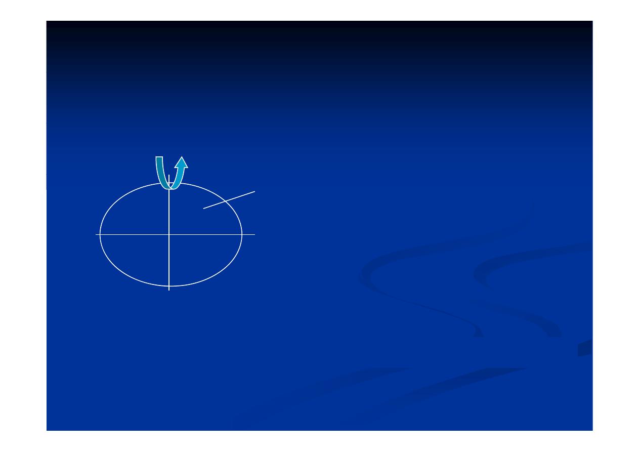
The centrifugal acceleration

•The centrifugal force acts on the mass of the
earth as a consequence of its rotation around

earth as a consequence of its rotation around
its axis (Fig. 1).

•This force is proportional to the radius of
rotation “l” and the square of the angular

rotation l and the square of the angular
velocity “ω”

•It can be written as:

P = l . ω

. m

When

m = 1 gr.

We obtain the centrifugal acceleration.

P = l . ω

•The component of “P” along “F ” will have the form:

•The component of “P” along “F

” will have the form:

P = l . ω

. cos φ …… (3)

( )

Where “φ” is the latitude of the area at which gravity
is measured

is measured

Pole P

= Zero ( cos 90 = 0)

= l . ω

. cos φ

Equator P

=l .

( cos 0=1)

Fig.(1):Variation of centrifugal and attraction forces.

٠١

The Gravitational acceleration

e G a tat o a acce e at o

•The Gravitational acceleration “ g “ is the sum
of attraction acceleration F

and centrifugal

of attraction acceleration F

and centrifugal

acceleration P

g = F

+ P

g = -f . M /R

+ l . ω

. cos φ…..….…(4)

١١

•In the “CGS” units system , the acceleration

developed by a mass of one gram through the

i t k

action of a force of one dyne is taken as the
unit of gravitational acceleration and is called

unit of gravitational acceleration and is called
“gal” ( in the honors of Galileo , who first
measured the force of gravity)

gal = dyne/gr = gr . cm/sec

. gr = cm/sec

٢١

it “

l”

•In gravity prospecting smaller units “mgal”

which is equal to 0.001 gal is always used.

•The gravitational acceleration on the earth's

The gravitational acceleration on the earth s

surface varies between about 978 gals at the
equator and 983 gals at the poles.

٣١

f t

d i

it ti

•The

factors

reducing

the

gravitational

acceleration at equator are:

•Centrifugal force varies from zero at the poles

to about 3.4 gals at the

equator. This

variation is the main cause of the normal

variation is the main cause of the normal
variation of the gravitational acceleration from
the equator to the poles

the equator to the poles.

•The flattening in the polar regions of the earth

•The flattening in the polar regions of the earth
also contribute to this variation.

٤١

Gravitational potential and equipotential surfaces

•Gravitational potential is a continuous function, the

derivatives of this function along the directions X, Y, and
Z are the projections of gravity in these directions

Z are the projections of gravity in these directions.

•The gravitational potential “W” is the sum of the

potentials of attraction “V” and centrifugal force “U”.

V = f . m / r

U = ½ . ω

. l

W = f m / r + ½ ω

(5)

So,

W = f . m / r + ½ . ω

. l

………..….(5)

٥١

Potential field properties

•

It can be easily shown that the function “W” satisfies
the following:

the following:

1. Its derivatives along certain directions are the

it ti

components of gravitational acceleration along these
directions.

2. The change of potential (dW) when a mass is moved

from point to another (ds) is equal to the work

( )

expended in the movement.

i t l

t d

t id

3. For a point located outside attracting masses , the sum

of the second vertical derivatives of the attraction

t ti l l

di t

٦١

potential along the axes of orthogonal coordinates is
zero.

1- Its derivatives along certain directions are the

it ti

components of gravitational acceleration along these
directions.

δW/δx = F1.cos (F1,x) + P1.cos (P1,x) = F1x+P1x

δW/δy = F1.cos (F1,y) + P1.cos (P1,y) = F1y+P1y

δW/δz = F1.cos (F1,z) + P1.Zero = F1z

Where F1x, F1y, F1z, P1x and P1y are projections of
the strength of the attraction and centrifugal forces
respectively

٧١

respectively.

2- The change of potential (dW) when a mass is moved
from point to another (ds) is equal to the work expended

from point to another (ds) is equal to the work expended
in the moment.

dW = F dS

dW = F

. dS

Where

“F

” is the field strength and

“dS” is the elementary movement of mass

If th

i t i

d i

di l

t th

•If the point is moved in a direction perpendicular to the
direction of the force “F” dW = 0. Such a surface is called
equipotential surface because of the constancy of
potential on it.

potential on it.

•In the case of displacement of a point mass along the line

٨١

of action of the force “F” , then

dW = F . ds

3- For a point located outside attracting masses , the sum
of the second

derivatives of the attraction potential

along the axes of orthogonal coordinates is zero

along the axes of orthogonal coordinates is zero
(Laplace`s theorem)

v/δx

+ δ

v/δy

+ δ

v/δz

= zero

•When the point being attracted lies inside the attracting
masses, the Laplace equation leads to the equation

Poisson`s equation

/δ

4 f

v/δx

+ δ

v/δy

+ δ

v/δz

= - 4 π f σ

Where “σ” is the mass density

٩١

Where σ is the mass density

•If we are concerned with the gravitational potential,

W = f m / r + ½ l

. ω

•The Laplace`s equation will be :

W/δx

+ δ

W/δy

+ δ

W/δz

= 2ω

And Poisson`s equation will be:

And Poisson s equation will be:

W/δx

+δ

W/δy

+δ

W/δz

=-4 π f σ +2ω

٠٢

Normal Gravitational Field

a G a tat o a

e d

•The values of gravity depend on the latitudes.

When the earth is considered as an ideal

When the earth is considered as an ideal
ellipsoid , then the gravitational field is known
as the normal field .

١٢

•Clairaut`s theorem gave firstly the essential
correlation between the figure of the earth

correlation between the figure of the earth
and the distribution of gravity on it, given in
the form:

g = g

( 1 + β sin

φ – β` sin

2 φ )

β = 5/2 q- α , β` = 1/8 α

+1/4 α β

٢٢

Where:

is the equatorial gravity

is the latitude of the locality.

α = a-b/a

is the flattening of the earth, a and b

are semimajor and semi minor axes of the earth.

q = ω

l / g

is the ratio of centrifugal force to

ω l / g

is the ratio of centrifugal force to

gravity at the equator.

٣٢

•If the earth is taken as triaxial ellipsoid a term

it d i

dd d t th l t

depending on longitudes is added to the last equation

g = g

[1+ β sin

φ – β`sin

2φ + β``cos

φ cos

(λ- λ

)]

•The Clairaut theorem is employed to determine the

flattening of the earth from known values of gravity and
to calculate theoretical gravity values for points at known

to calculate theoretical gravity values for points at known
latitudes.

٤٢

•The formula with numerical coefficients describing the

gravitational field, is called the standard gravity
formula

formula.

•Only two formulae have found practical application,

Helmert`s and Cassins formulae.

٥٢

Th H l

` f

l f

bi i l lli

id i

•The Helmert`s formula for biaxial ellipsoid is;

g = 978.03 (1+0.005302 sin

φ – 0.000007 sin

2φ )

g 978.03 (1 0.005302 sin φ 0.000007 sin 2φ )

•The Helmert`s formula for triaxial ellipsoid is:

978 052 [ 1+0 005285 i

0 0000007 i

2 +

g =978.052 [ 1+0.005285 sin

φ– 0.0000007 sin

2φ +

0.000018 cos

φ cos2(λ- 17°)]

0 0000 8 cos φ cos (

7 )]

•The Cassins formula for biaxial ellipsoid is:

978 049 (1+0 0052884 i

0 0000059 i

2 )

٦٢

g =978.049 (1+0.0052884 sin

φ– 0.0000059 sin

2 φ)

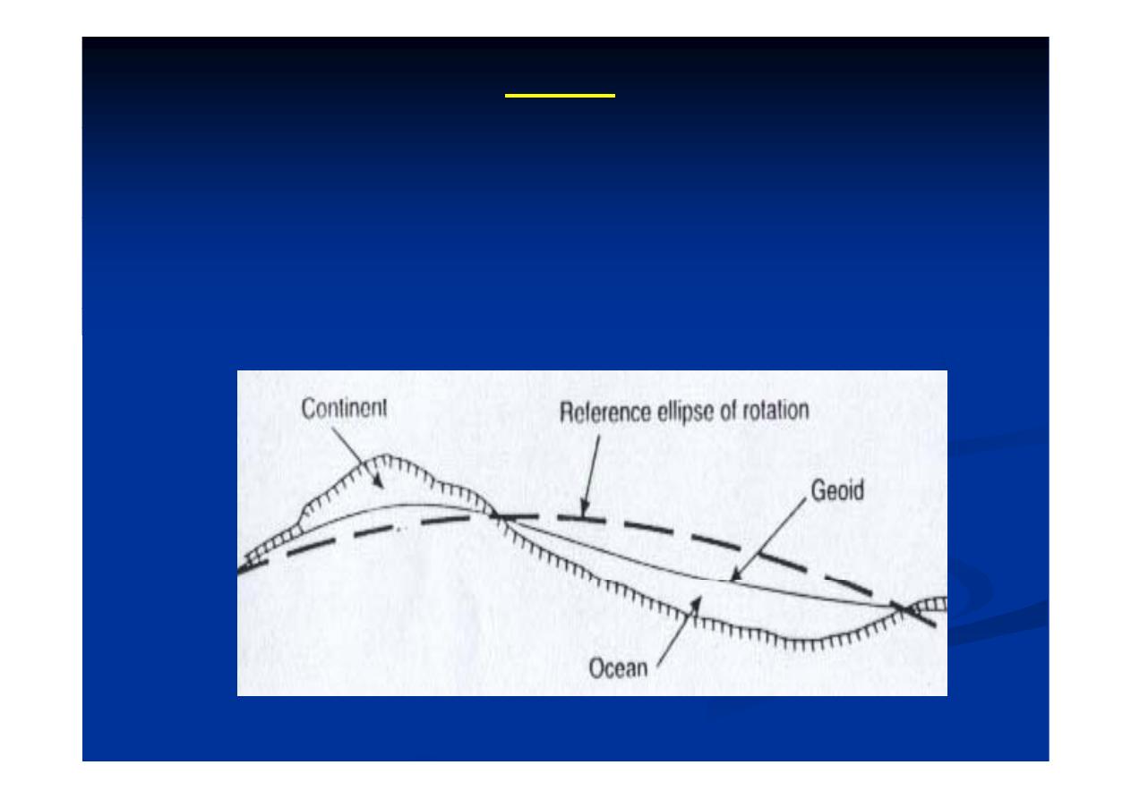
Geoid

•It is an equipotential surface that coincide with the level
of oceans and seas.

•The direction of the force of gravity at any point on the
Geoid is normal to this surface

Geoid is normal to this surface.

٧٢

Fig.(3):The Geoid

•The geoid appears as a convenient surface for

l i

i Fi (3)

relating all measured values of gravity Fig.(3).

I f t it i diffi lt t

•In fact it is difficult to compare the values of
gravity measured at different elevations; but

;

when they are reduced to the geoid surface,
they appear to be at one level which enable us
to compare them

to compare them

٨٢

Measurements of gravity acceleration

•There are three methods for determining gravity:

-The pendulum method.

-The measurement of velocity of a freely falling body.

- The weighing method (by means of a spring balance).

٩٢

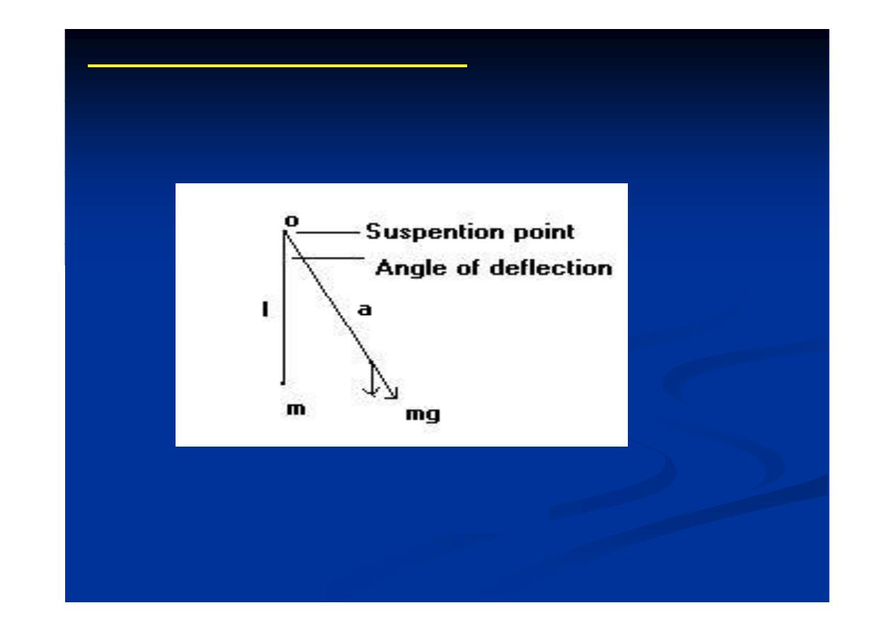
1-The Pendulum method:

d l

th d i th fi t

th d

•The pendulum method is the first used method
for the measurement of gravity (Fig.4).

Fig.(4): The pendulum

٠٣

The methods of gravity determination by using

The methods of gravity determination by using
the pendulum can be classified into:

•The absolute method, in which determinations

of gravity at any point from measured
oscillation periods and pendulum length is
done

(irrespective

the

place

measurement).

•The used equation is (T =π √ l / g

)

١٣

•The relative method, in which the increment

i i i

of gravity from the initial point to the
observation point is determined from the

obse vat o

po t s dete

t e

increment of the oscillation period of the
pendulum

•The used equation is (Δg/g

= 2ΔT/T

)

٢٣

2- Determination of gravity by measuring the

velocity of freely falling bodies:

•This method enables gravity “g” to be determined by
the formula:

the formula:

S = g . T

/ 2

Where

“S” is the path traversed by the freely falling body

“T” i h i

b h f lli

b d

“T” is the time taken by the falling body

٣٣

3- Gravity determination by weighing:

•This method is based on compensating the force F1= mg
by a mass raised in the field of force by the elastic

by a mass raised in the field of force by the elastic
strength of a wire string or pressure of an elastic gas.

•Consider a mass “m” is suspended from an elastic
spring having an initial length “l ” and loaded length

spring having an initial length l

and loaded length

“l”. Then , according to Hooke`s law,

mg = τ ( l l )

mg = τ ( l – l

)

Where “ τ “ is the stretching of the spring

٤٣

Where τ is the stretching of the spring.

•From the last relation we find that the increment of

•From the last relation we find that the increment of
length is proportional to the change of gravity, then:

m Δg = τ Δ l

Δg = τ / m Δ l

Δg = K Δ l

Where “K” is the spring constant

•This method is always relative, i.e. all instruments
for measuring gravity by weighing (gravimeters)
enable the variations of gravity to be measured with

enable the variations of gravity to be measured with
respect to some initial value.

٥٣

Reduction of Gravity Data

•The gravity values cannot be compared in the form in
which they are obtained.

•The corrections of obtained gravity data enable it to be
reduced to a certain standard surface (sea level) for

reduced to a certain standard surface (sea level) for
comparison.

-The observed values of gravity depend on:

•The location of the station on the earth's surface,
i.e. its coordinates and elevation.
•The density distribution within the earth.

•The topography of the surrounding localities

٦٣

•The topography of the surrounding localities

•To obtain the part of the observed gravity

values relating to the density variations that
interest us we divide its values into;

interest us, we divide its values into;

- A part that varies regularly reflecting the

figure of the ideal earth,

- And into anomalies that reflect the internal
structure of the upper part of the earth.

٧٣

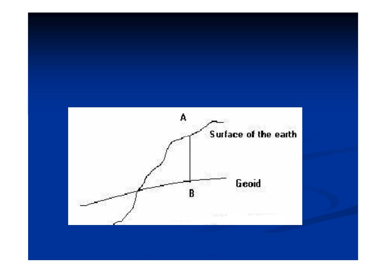
•The actual value of gravity is observed on the surface
of the earth at point (A), the standard value is given for
point (B) on the surface of the Geoid (Fig. 5).

point (B) on the surface of the Geoid (Fig. 5).

٨٣

Fig.(5):Diagram of surfaces in gravity reductions

•In order to obtain the gravity it is necessary
to reduce the observed value to the surface of
the geoid.

•The

gravity anomaly is obtained by

subtracting the standard value for the ideal
earth from the actual gravity value observed

at the station

Δg = g

– g

٩٣

1- Drift correction:

•All gravity instruments have certain amount

f d ift

i ti

t th t th

of drift or time variation due to that the spring
and the associated mountings are not perfectly
stable.

•These may cause changes in meter reading
which are larger than those due to the small
gravity differences being measured.

The field

ork m st be cond cted in a

•The field work must be conducted in a way
that this drift can be determined and

٠٤

corresponding corrections made.

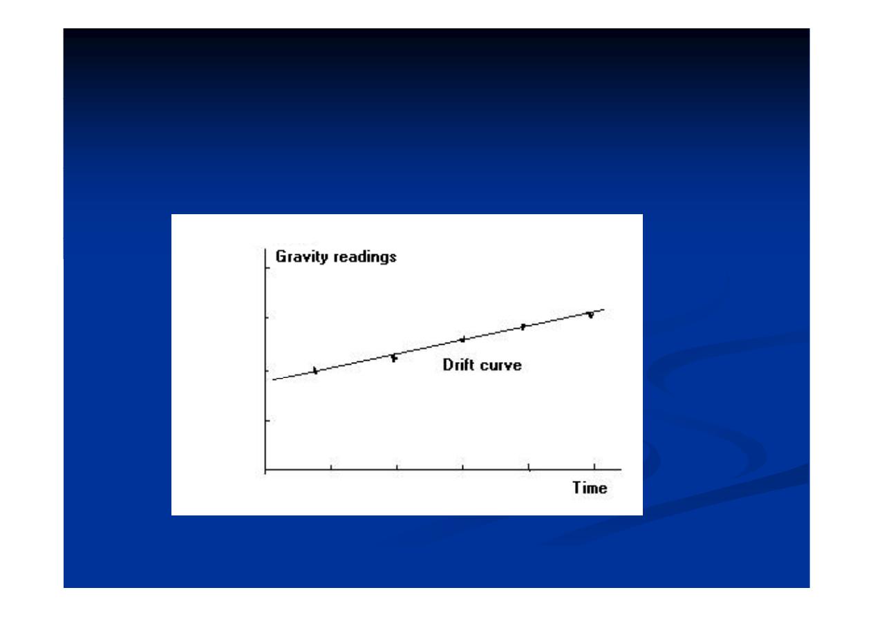
•Drift

curves

are

obtained

repeated

occupation of a single field station at intervals
during the day (see Fig. 6).

during the day (see Fig. 6).

١٤

Fig.( 6 ):Gravimeter drift curve

2 Earth Tidal Correction:

2- Earth Tidal Correction:

•The changes in gravity caused by movement of

the sun and moon have amplitudes as large as
0 3 mgal They depend on latitude and time

0.3 mgal. They depend on latitude and time.

•The changes in gravity can be calculated

theoretically for any time and place.

•It is not practice to obtain the correction
directly , this is because the variation is smooth

y ,

and relatively slow., So it is easily taken out in
the instrument drift correction

٢٤

the instrument drift correction.

3 El

3- Elevation Correction:

•Correction to gravity values which must

Correction to gravity values which must

be made due to the differences in elevations
t k

f t

ff t

take care of two effects:

A- The free air effect

B- The Bouguer effect

٣٤

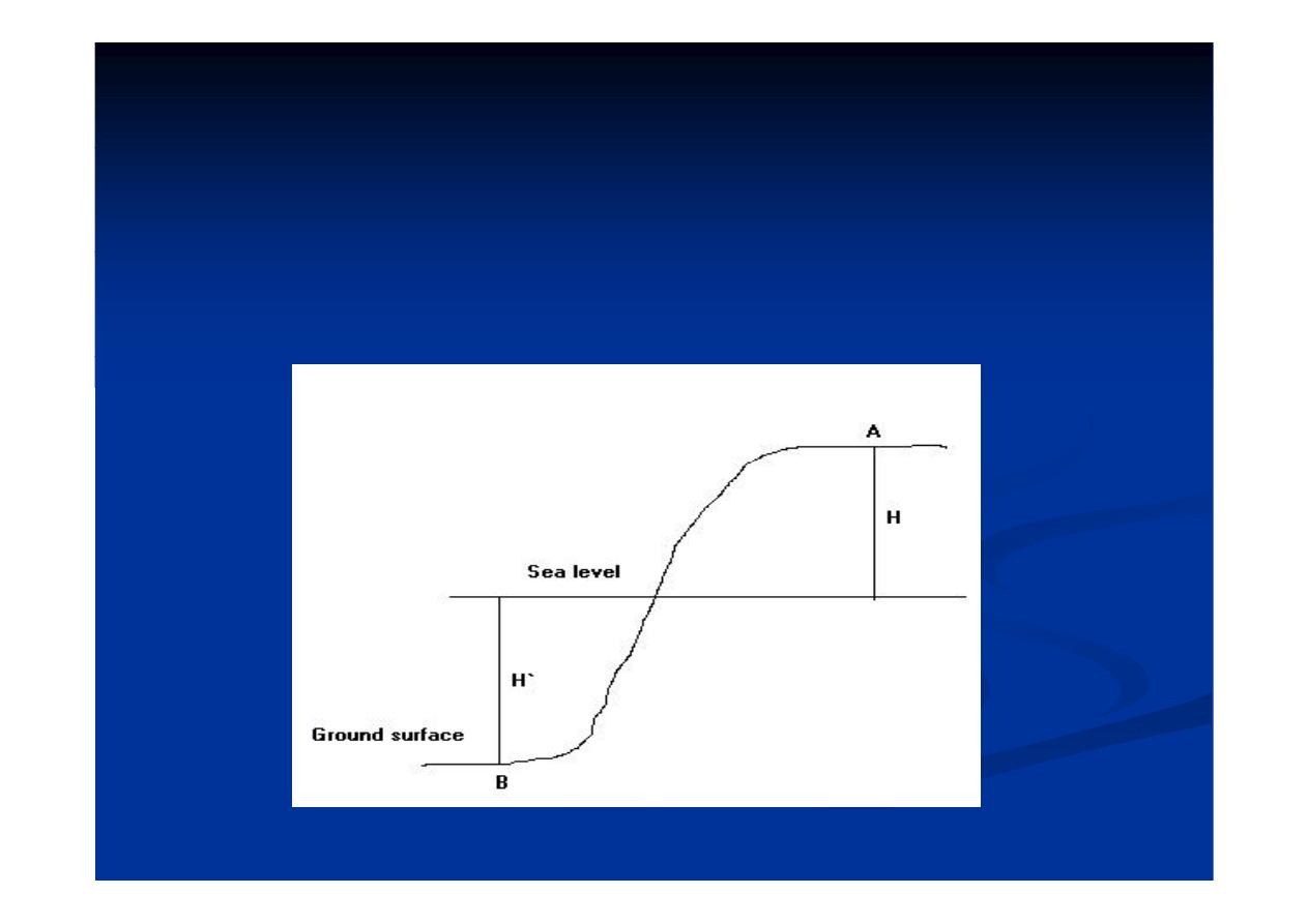
A- Free air correction:

ti l d

ith i

•The vertical decrease of gravity with increase of
elevation is taken care of by the free-air correction. The

f f

“d f”

l l t d

value of free-air correction “dgf” can be calculated
(Fig. 7) :

= - 2 g / R H ……….(42)

٤٤

Fig. (7 ):Free-air effect

•If we take;

-The mean radius of the earth “R”=6.367 x
10

cm, gravity at sea level and at latitude 45

10 cm, gravity at sea level and at latitude 45
g = 980.629 gals, and the elevation H = 1 cm ,

= - 2 x 980.629/6.367x10

0 3086 10

-0.3086x10

-5

gal/cm =

- 0.3086 mgal / m = - 0.09406 mgal / ft

٥٤

•The corrections can be made to any arbitrary
reference or datum level, or it may be made to
sea level.

l i l hi h

•Since a station at a relatively higher elevation
has a lower gravity (because it is farther from
the center of the earth), the correction must be
added to it.

added to it.

• While the corrections must be subtracted
from stations at lower elevations than the
reference level (Fig. 7).

٦٤

reference level (Fig. 7).

B- Bouguer Correction:

•The Bouguer correction take care to the attraction of
the material between a reference elevation and that of

the material between a reference elevation and that of
the individual station.

•Considering the material as an infinite horizontal
slab, the gravity attraction for a point on the surface

slab, the gravity attraction for a point on the surface
of a slab of thickness “h” and density “σ “(Fig. 8) is:

= 2 π f σ h

Which for f = 6.6732 x 10

-8

gives:

Which for f 6.6732 x 10

gives:

= 0.04193 x σ mgal/ m

٧٤

= 0.01278 x σ

mgal/ ft

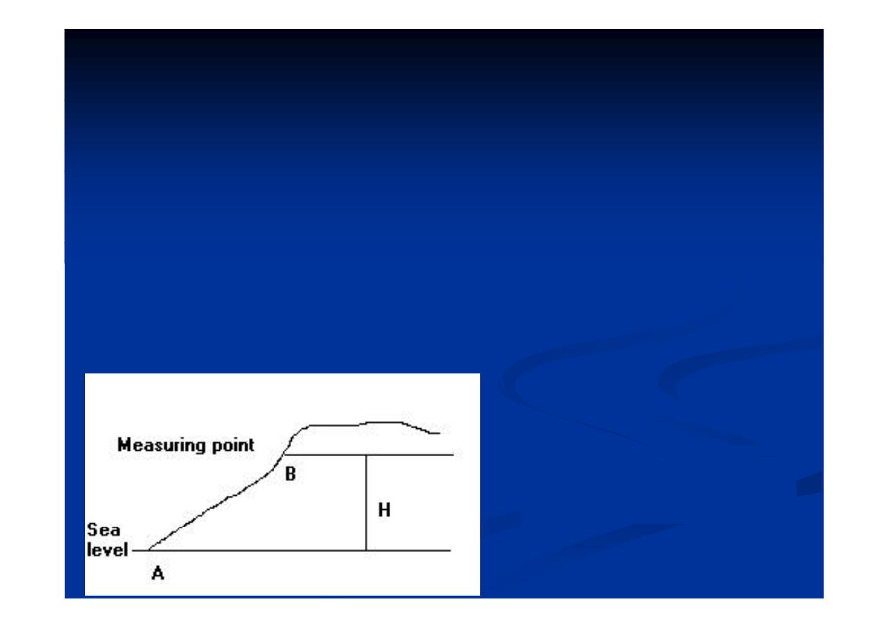
•In a station “B” higher than the reference elevation “A”

its gravity value is increased because of the attraction

, its gravity value is increased because of the attraction
of the slab of material between it and the reference level
and the correction is subtracted (Fig 8)

and the correction is subtracted (Fig. 8).

•If the station is lower than the reference elevation , its
gravity value is decreased because of the lake of
attraction of the absent material between it and the
reference level and the correction is added.

Fig.(8):The Bouguer

gravity effect

٨٤

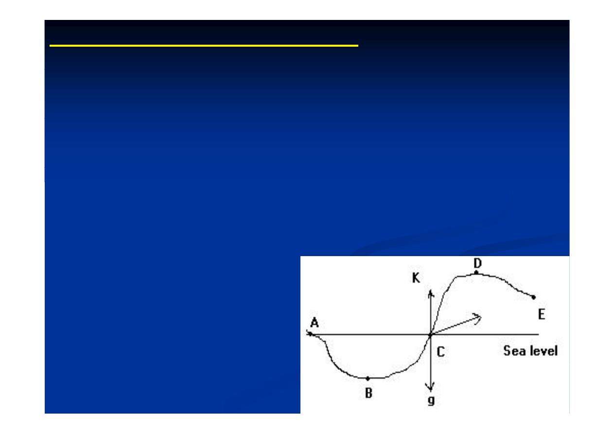
4-Topographic (terrain) correction:

•Topographic correction always reduce the observed
gravity value irrespective of whether there is a rise or a
d

t ti

depression near the gravity station.

•

The presence of extra mass “CDE” lying higher than the

y g

observation point will give rise to an additional force
directed towards the mass. The vertical component “CK”

of this force will reduce the value of “g” (Fig. 9).

Fig.(9): Gravity effect

of relief

٩٤

of relief

•The lake of mass in the region “ABC” will also bring
down the value of “g” with respect to the value that
would be obtained if the entire region below the point
of observation were filled

•In practice topographic corrections are calculated

•In practice topographic corrections are calculated
from zone charts, nomograms and terrain correction
tables that enable us to fined the correction from

tables, that enable us to fined the correction from
topographic maps for any point at which gravity is
measured

measured.

٠٥

Interpretation of Gravity Data

•The interpretation of gravity data involves qualitative

tit ti

i t

t ti

and quantitative interpretation.

1-Qualitative Interpretation of Gravity Data:

•The result of gravity surveys (after the corrections) is
the Bouguer gravity anomaly map.

the Bouguer gravity anomaly map.

•The objective of gravity interpretation is to translate

gravity data to geological terms, to give the features of the
subsurface structures

subsurface structures.

•From the various characteristics of the map, the

١٥

amplitude, shape and the sharpness of the anomalies.

•The location and form of the structure which

•The location and form of the structure which
produce the gravity disturbance can be deduced.

•The

magnitude of a gravity anomaly is

important because the size of an anomaly is

important because the size of an anomaly is
proportional to the size of the structure and the
d

density contrast.

•The direction of elongation of iso anomaly

•The direction of elongation of iso anomaly
contours of gravity suggests the direction of the
l

length

the

structure

causing

them.

Concentrated masses produce approximately

٢٥

circular anomaly patterns.

2-Quantitative Interpretation of Gravity Data

I i

h i

i ld

It is the interpretation of gravity data to yield
the numerical characteristics of the body being
studied (depth and dimensions).

•The quantitative interpretation of gravity data
involves:

A - Anomaly separation and filtration.

B- Calculation of gravity effects of different

causative bodies

٣٥

causative bodies.

REFERENCES

-Nettleton, L.L., (1976):

Gravity and Magnetic in oil

prospecting. McGraw Hill Book Co., New York: 464P

Sazhina N and Grushinsky N (1971):

Gravity

-Sazhina, N. and Grushinsky, N. (1971):

Gravity

Prospecting. Mir Publishers, Moscow, 491 P.

-Dobrin and Savit (1986):

Introduction to geophysical

prospecting 4th Ed. ,Mc Graw Hill book company,
New York, 867p.

Telford W M Gildart L P Sheriff R E and Keys

-Telford, W. M., Gildart, L. P., Sheriff, R. E., and Keys,

D. A. (1990):

Applied Geophysics , Cambridge

University Press 770 P

٤٥

University Press, 770 P.

٥٥