COULOMB’S LAW AND ELECTRIC FIELD
INTENSITY
2.1 The Experimental Law Of Coulomb
• Coulomb stated that the magnitude of the force
between two very small objects separated in free
space by a distance, which is large compared to
their size, is proportional to the charge on each
and inversely proportional to the square of the
distance between them.
• If point charges Q1 and Q2 are separated by
distance R, then the magnitude of the force
between them is:
1
where the new constant Є
0
is called the permittivity
of free space (
(
سماحية الفضاء الحرand has magnitude
()قيمة, measured in farads per meter (F/m),
The constant of proportionality k is written as
2
• Coulomb’s law is now
• In order to write the vector form of the force,
we need the additional fact that the force acts
along the line joining the two charges. If the
force F
2
on charge Q2 is required, then
3
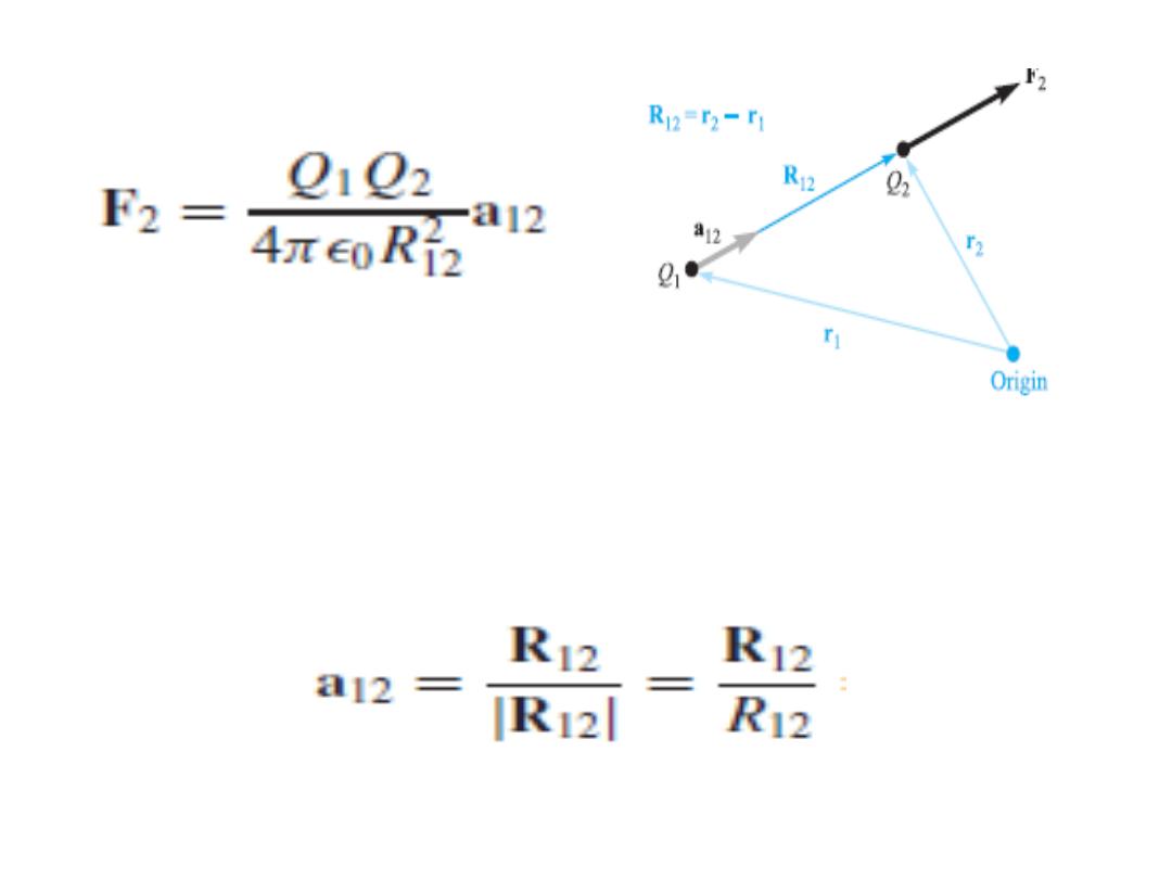
where a
12
is a unit vector ( )وحدة متجهin the
direction of R
12
, (
تبدأ ب
1
وتنتهي ب
2
) or:
4
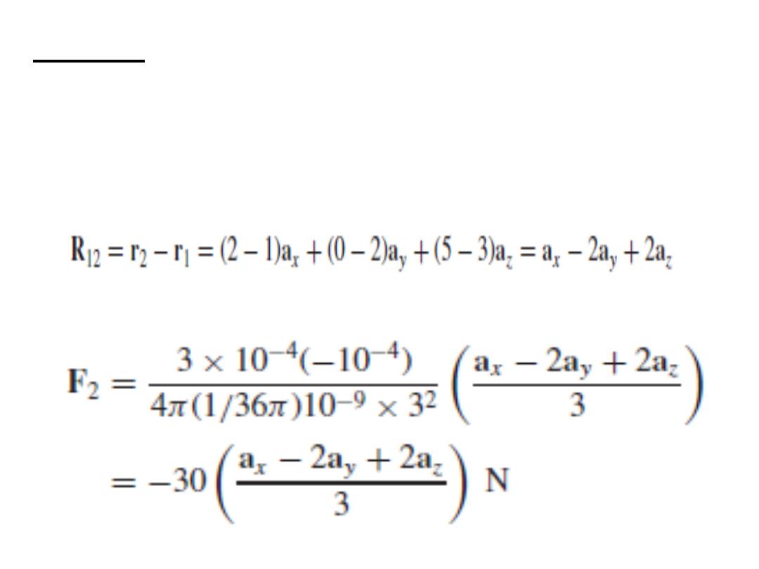
Example: A charge of Q1 = 3 × 10⁻⁴ C at M(1, 2, 3) and a
charge of Q2 = −10−4 C at N(2, 0, 5) in a vacuum. Find the
force on Q2 by Q1.
Solution: We have
5
The magnitude of the force is 30 N, and the direction is
specified by the unit vector, which has been left in
parentheses ( )قوسينto display the magnitude of the
force.
The force on Q2 may also be considered as three
component (تابكرم) forces,
F
2
= −10a
x
+ 20a
y
− 20a
z
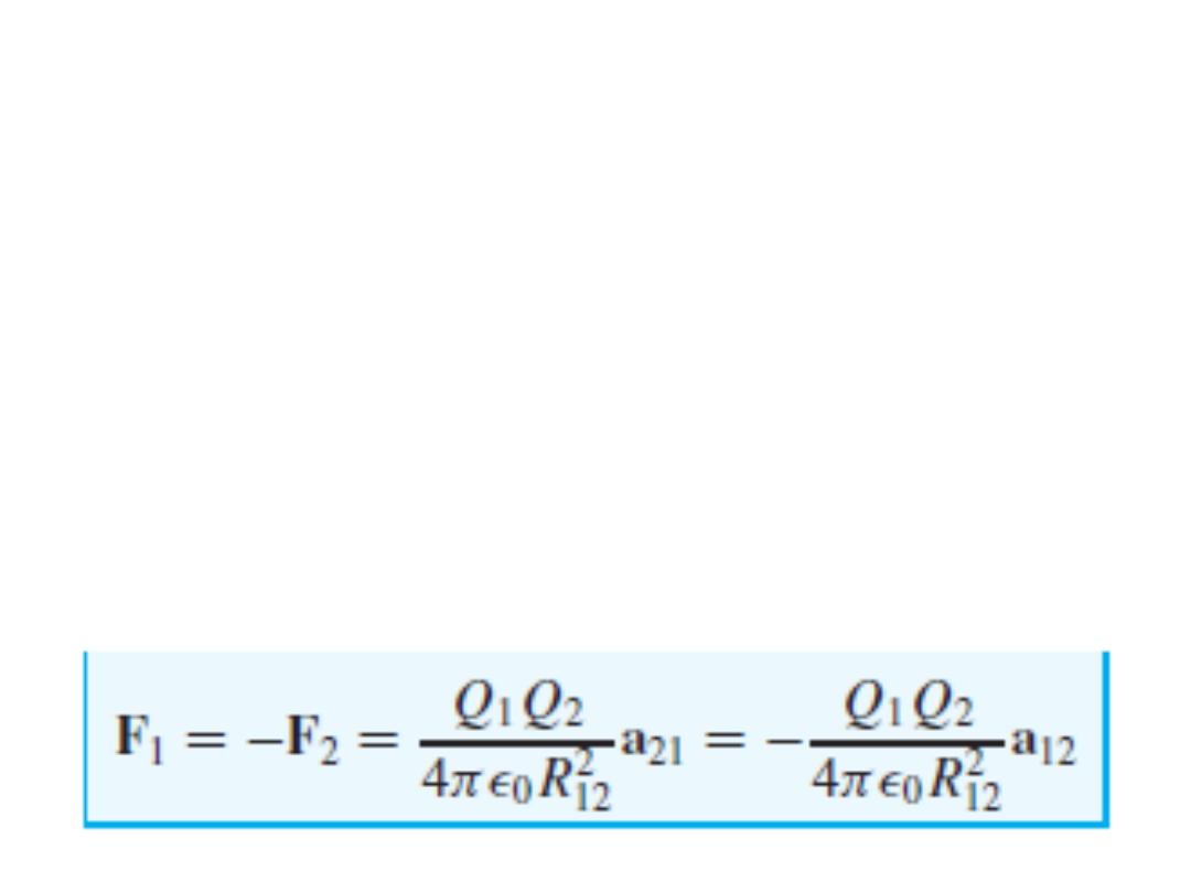
• We might equally well have written:
6
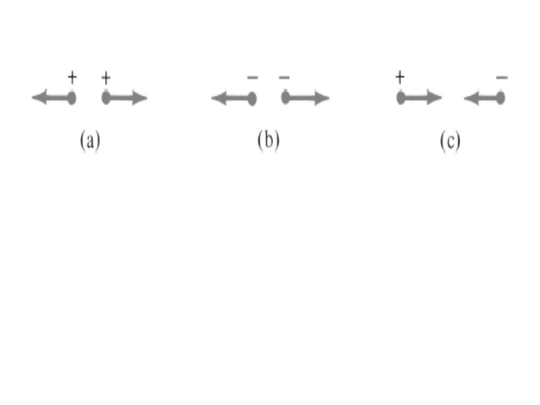
( )تجاذب( )تنافر( )تنافر
Repulsion Repulsion Attraction
7
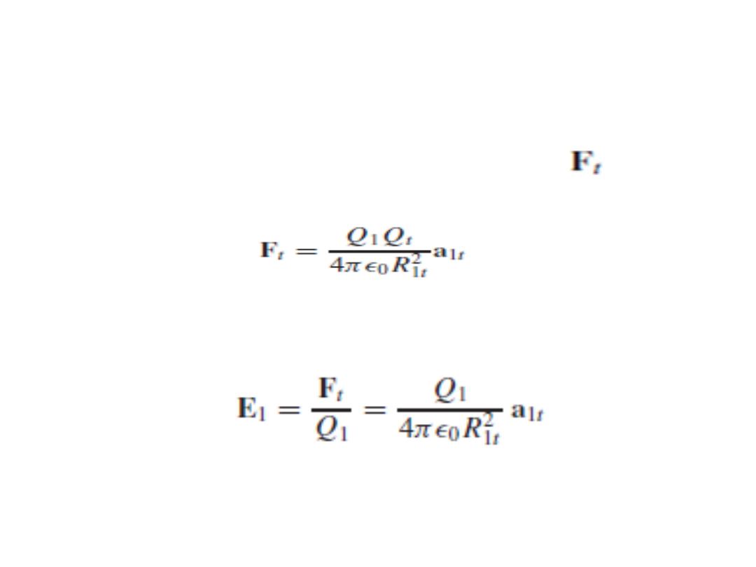
2.2 Electric Field Intensity
• If the second charge is called a positive test
charge
(شحنة أختبارية
) Q
t
, the force on it is given
by Coulomb’s law as:
• Writing this force as a force per unit charge gives
the electric field intensity, E
1
arising from Q
1
:
• The units of E is volts per meter (V/m).
8
• If we arbitrarily locate Q1 at the center of a
spherical coordinate system. The unit vector
a
R
then becomes the radial unit vector ar , and
R is r . Hence
• In this case, the electric field has a single
radial component.
9
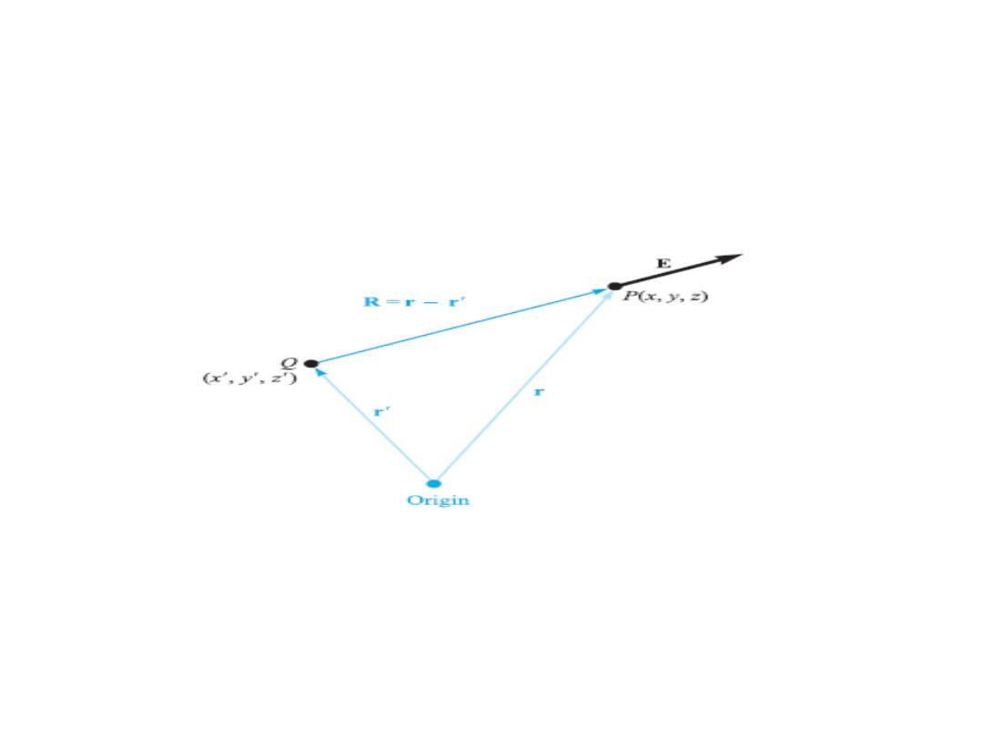
• For a charge Q located at the source point
r = xa
x
+ ya
y
+ za
z
,
as shown in the figure,
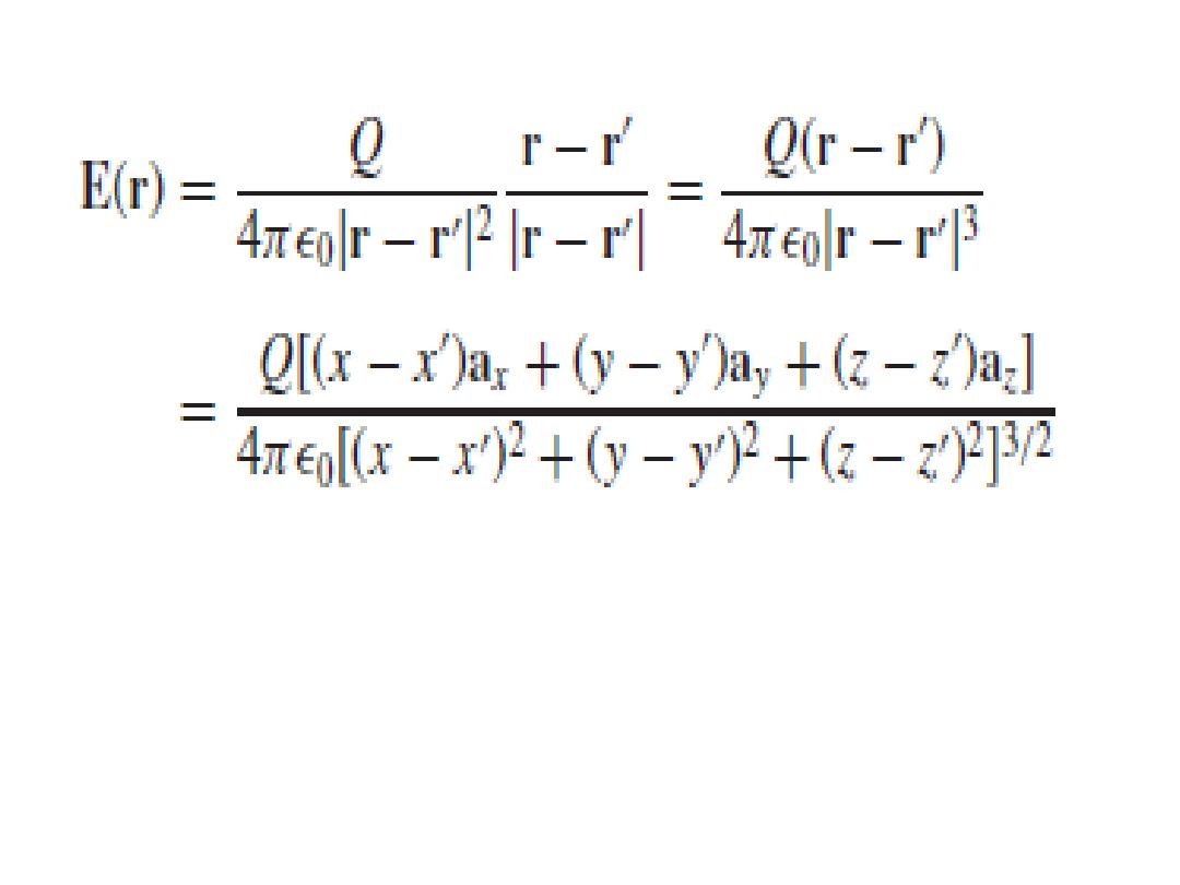
• we find the field at a general field point
r = xa
x
+ ya
y
+za
z
by expressing R as r-rʹ and then
10
11
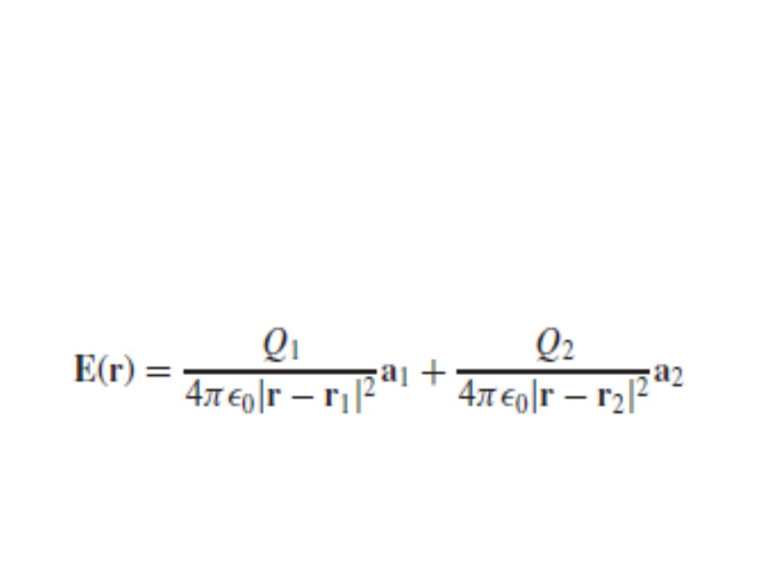
2.3 Electric Field of n point charges
• Because the coulomb forces are linear, the
electric field intensity arising from two
point charges, Q
1
at r
1
and Q
2
at r
2
, is the
sum of the forces on Q
t
caused by Q
1
and
Q
2
acting alone ()بمفردها, or:
• The vectors r, r
1
, r
2
, r − r
1
, r − r
2
, a
1
, and a
2
are shown in the figure.
12
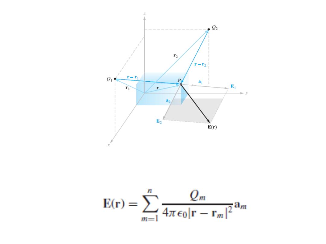
• If we add more charges at other positions, the
field due to n point charges is:
13
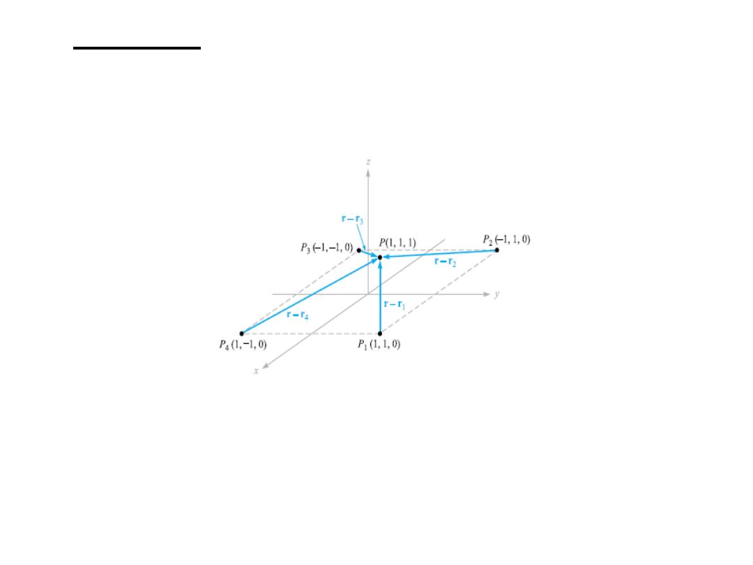
• Example: Find E at P(1, 1, 1) caused by four
identical ( )متشابه3nC (nanocoulomb) charges
located at P
1
(1, 1, 0), P
2
(−1, 1, 0), P
3
(−1,−1, 0),
and P
4
(1,−1, 0), as shown in the figure.
Solution: We find that r = a
x
+ a
y
+ a
z
,
r
1
= a
x
+ a
y
, and thus
r − r
1
= a
z
.
14
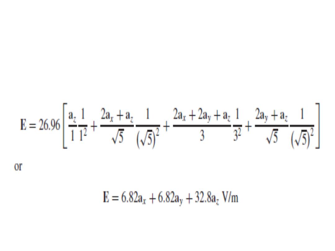
The magnitudes are: |r − r
1
| = 1, |r − r
2
| = √5, |r − r
3
|
= 3, and |r − r
4
| = √5 and
Q/4πϵ
0
= 3 × 10⁻⁹/(4π × 8.854 × 10−12) = 26.96 V.m,
we may now obtain:
15
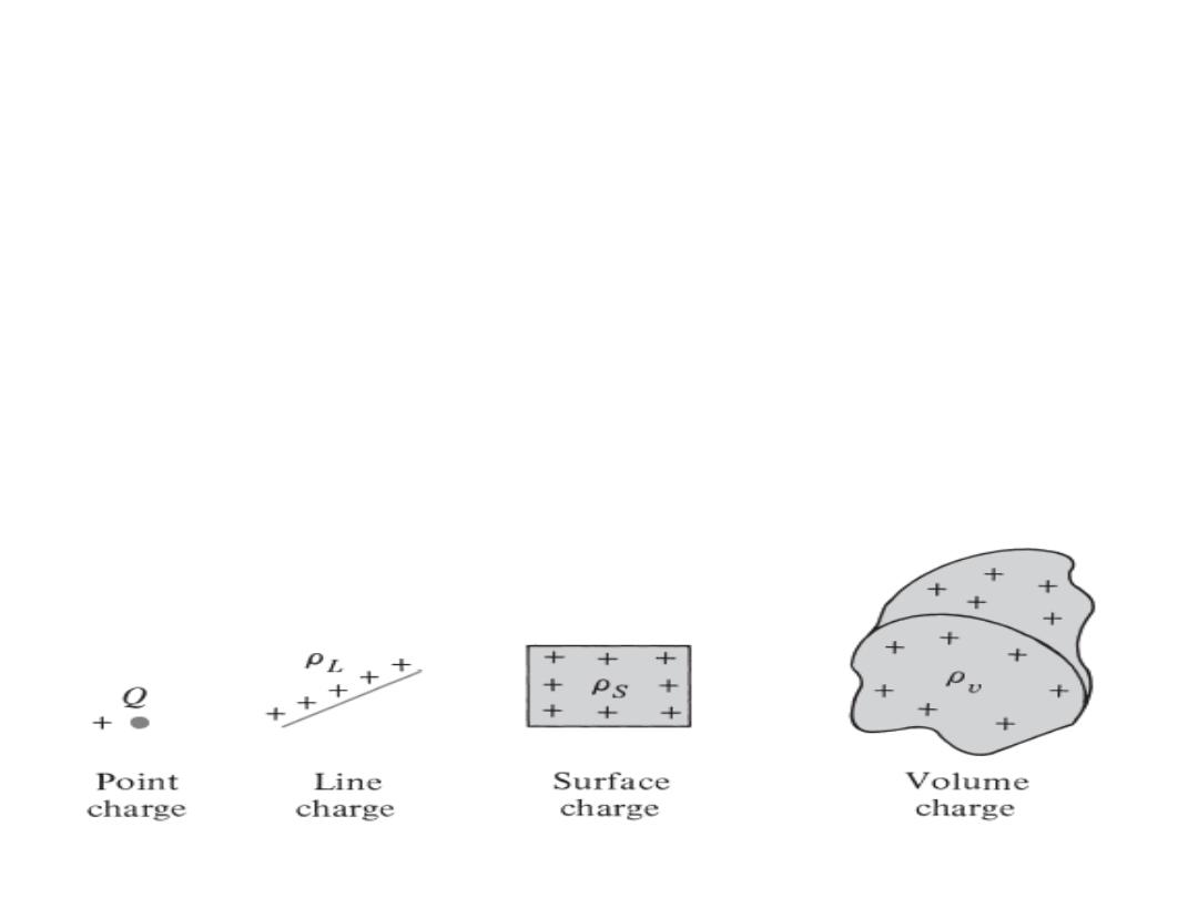
2.4 Electric Fields Due To Continuous Charge
Distributions
• It is customary to denote the line charge
density, surface charge density, and volume
charge density by ρ
L
in (C/m), ρ
s
in (C/m2),
and ρ
v
in (C/m3), respectively ( .)بالتعاقب
16
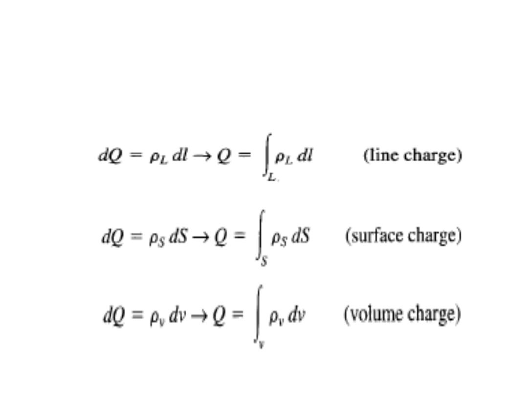
• The charge element dQ and the total charge Q
due to these charge distributions are obtained
as:
17

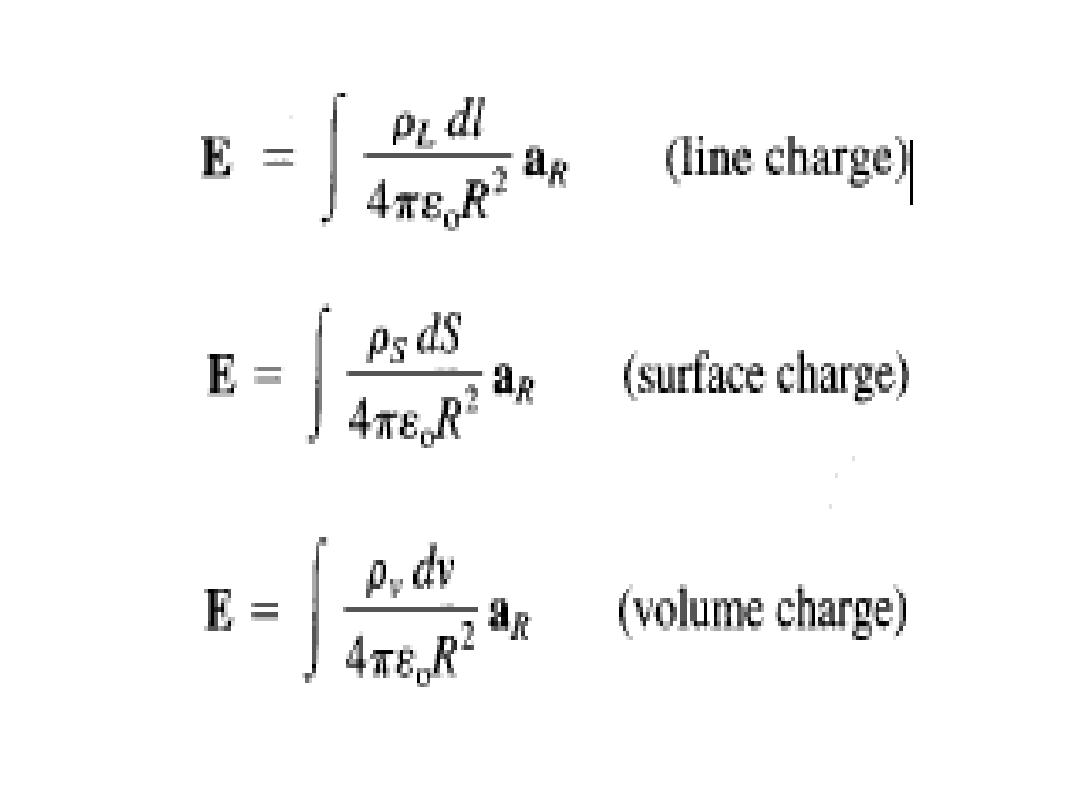
• The electric field intensity due to each of the
charge distributions ρL, ρs, and ρv may be
regarded as the summation of the field
contributed by the numerous point charges
making up the charge distribution. Thus by
replacing Q with charge element dQ = ρ
l
dl,
ρ
s
dS, or ρ
v
dv and integrating, we get:
18
19
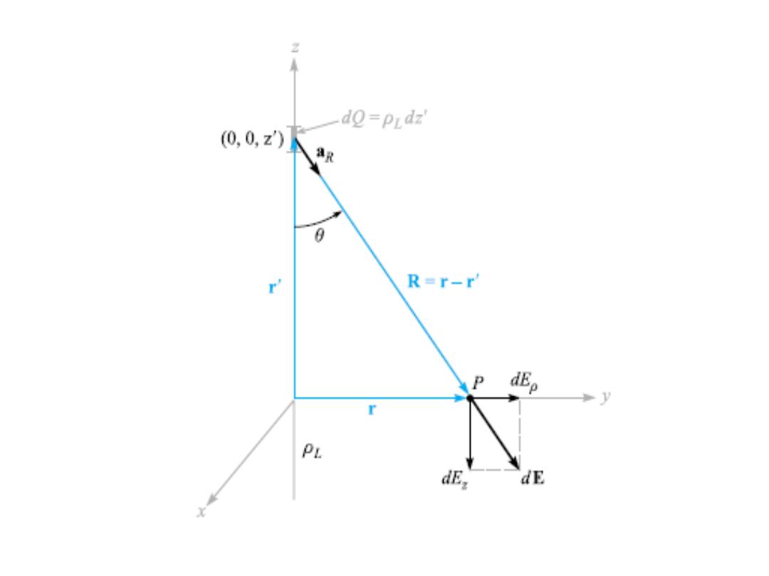
2.4.1
Field Of a Line Charge
• In this case, the charge is distributed along a
line with a line charge of density ρL C/m.
• Example: Assume a straight-line charge
extending along the z axis in a cylindrical
coordinate system from −∞ to ∞, as shown in
the figure. Find the electric field intensity E at
any and every point resulting from a uniform
line charge density ρ
L
.
20
21

• Each incremental length of line charge acts as
a point charge and produces an incremental
contribution to the electric field intensity
which is directed away from the bit of charge
(assuming a positive line charge).
• We choose a point P(0, y, 0) on the y axis at
which to determine the field.
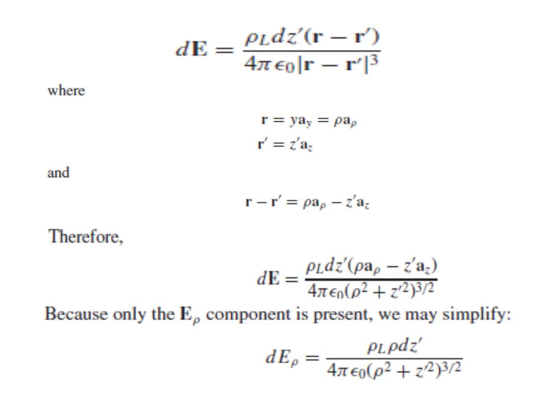
• To find the incremental field at P due to the
incremental charge dQ = ρ
l
dz, we have
22
23
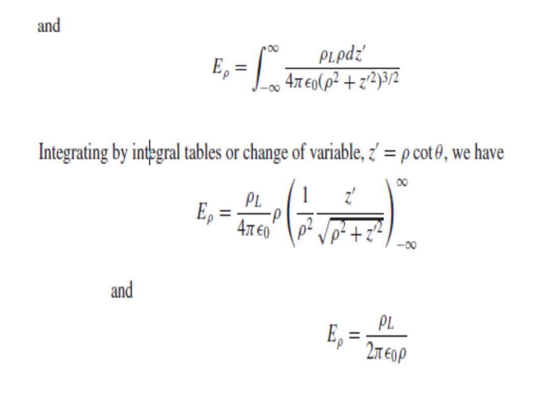
24
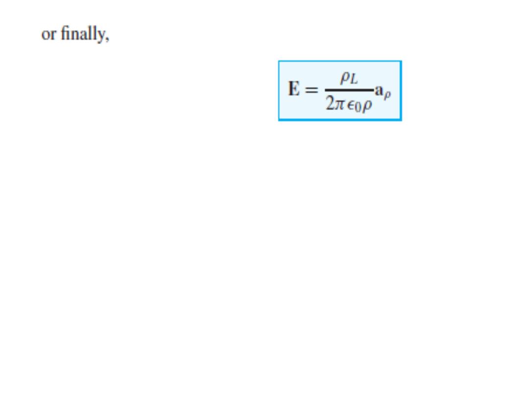
• We note that the field falls off inversely with the
distance to the charged line, as compared with
the point charge, where the field decreased with
the square of the distance.
• Moving ten times as far from a point charge
leads to a field only 1 percent the previous
strength, but moving ten times as far from a line
charge only reduces the field to 10 percent of its
former value.
25
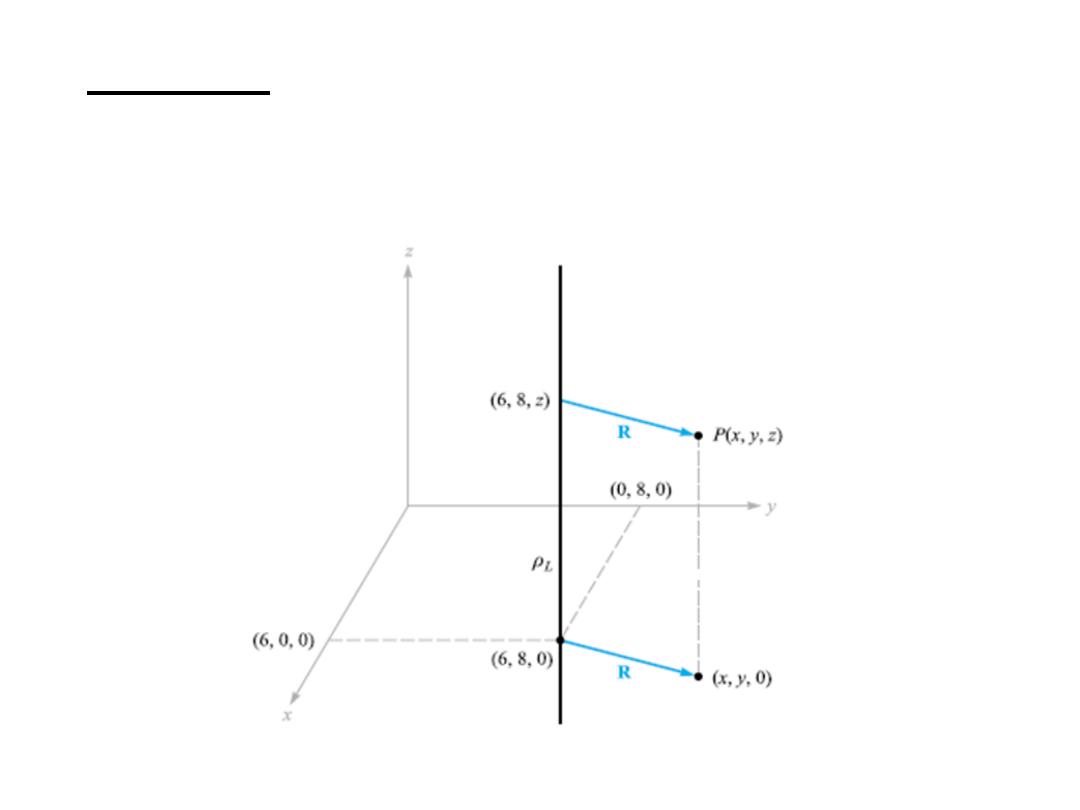
• Example: let us consider an infinite line charge
parallel to the z axis at x = 6, y = 8, shown in the
figure. Find E at the general field point P(x, y, z).
26
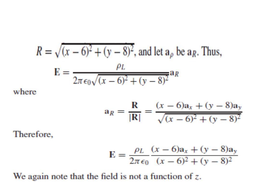
• We replace ρ by the radial distance between
the line charge and point P,
27

• Drill Problem: Infinite uniform line charges of
5 nC/m lie along the (positive and negative) x
and y axes in free space. Find E at: (a) P
A
(0, 0,
4); (b) P
B
(0, 3, 4).
• Ans. 45az V/m; 10.8ay + 36.9az V/m
28

2.5 Field Of A Sheet Of Charge
• Another basic charge configuration is the
infinite sheet of charge having a uniform
density of ρ
S
C/m2. Such a charge distribution
may often be used to approximate that found
on the conductors of a strip transmission line
or a parallel-plate capacitor.
• Static charge resides on conductor surfaces
and not in their interiors; for this reason, ρ
S
is
commonly known as surface charge density.
29
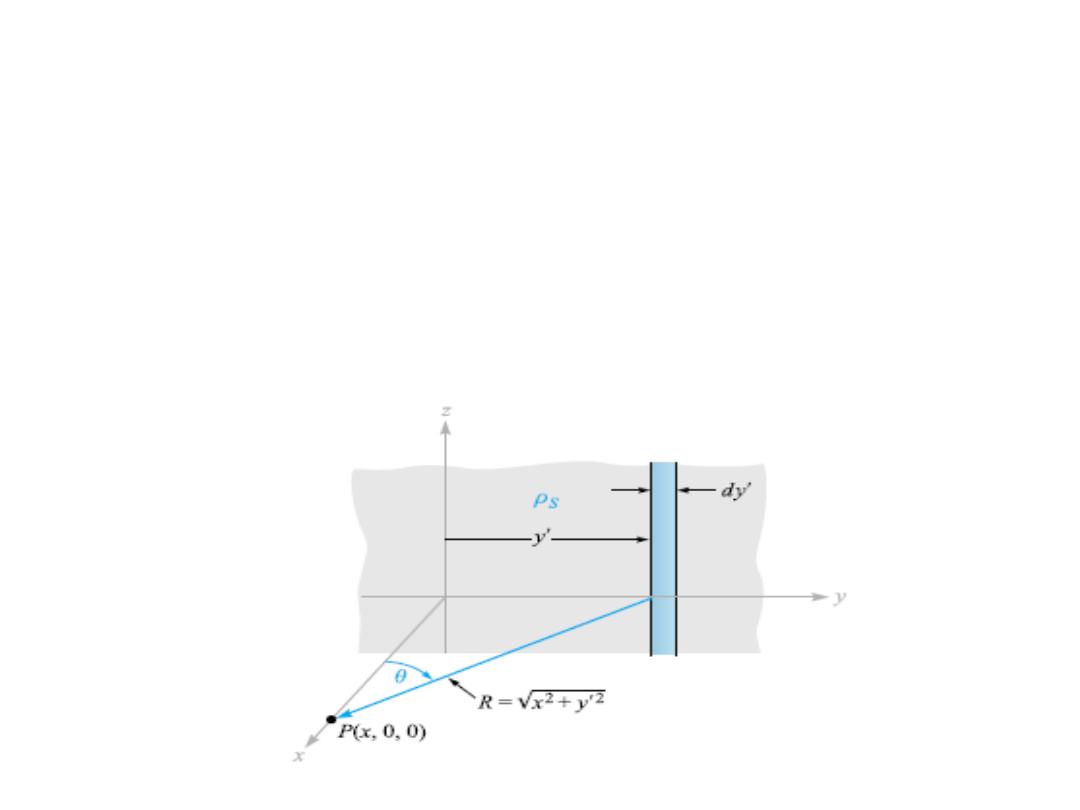
• Let us place a sheet of charge in the yz plane
and again consider symmetry as shown in the
figure.
• Let us use the field of the infinite line charge
by dividing the infinite sheet into differential-
width strips. One such strip is shown in the
figure.
30
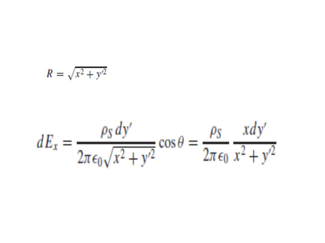
• The line charge density, or charge per unit
length, is ρ
l
= ρ
S
dy, and the distance from this
line charge to our general point P on the x axis
is . The contribution to Ex at P
from this differential-width strip is then
• Adding the effects of all the strips,
31
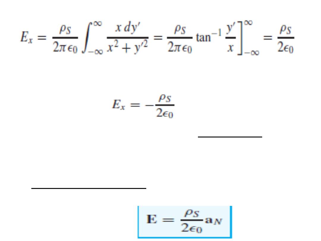
• If the point P were chosen on the negative x
axis, then
For the field is always directed away from the
positive charge. This difficulty in sign is usually
overcome by specifying a unit vector a
N
, which
is normal to the sheet and directed outward, or
away from it. Then
32
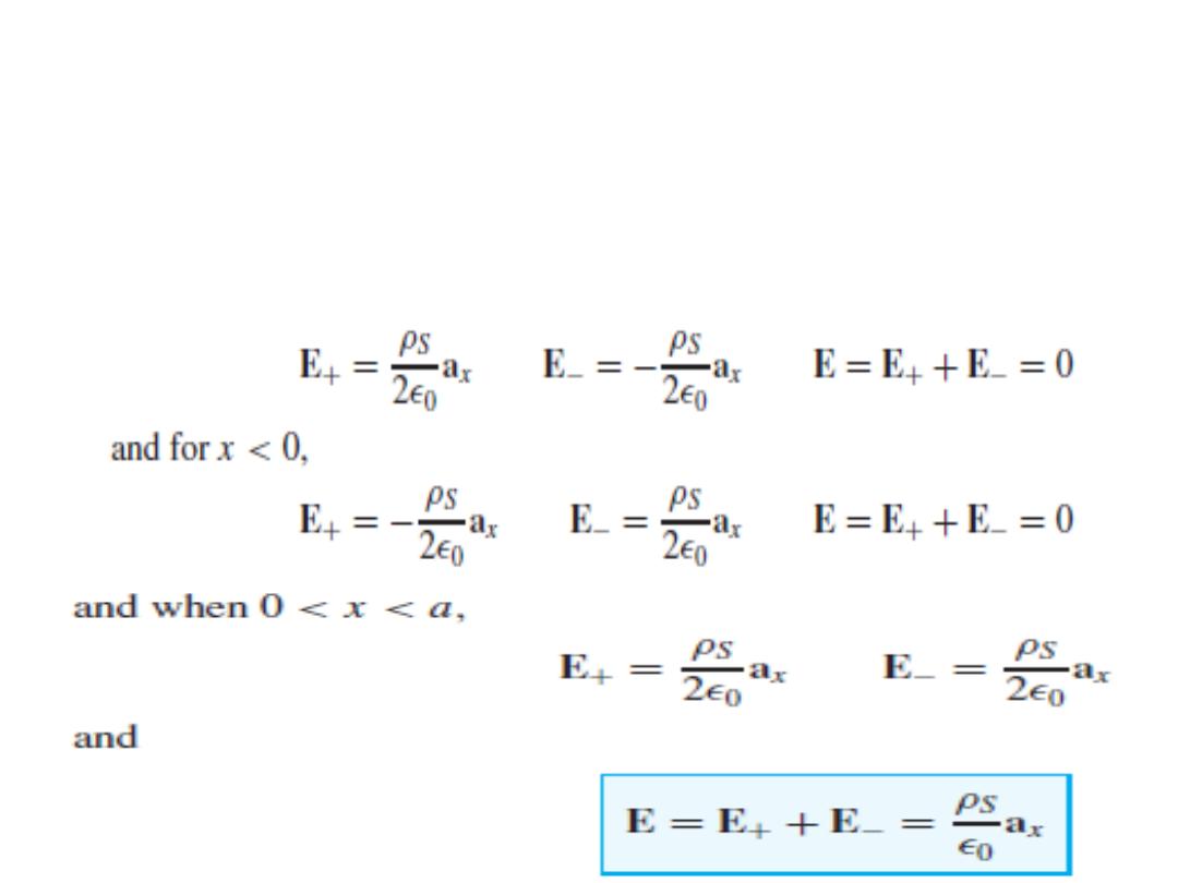
• If a second infinite sheet of charge, having a
negative charge density −ρS, is located in the
plane x = a, we may find the total field by
adding the contribution of each sheet. In the
region x > a,
33
• Drill Problem:
Three infinite uniform sheets of charge are located
in free space as follows: 3 nC/m2 at z = −4, 6 nC/m2
at z = 1, and −8 nC/m2 at z = 4. Find E at the point:
(a) PA(2, 5,−5); (b) PB(4, 2,−3); (c) PC(−1,−5, 2); (d)
PD(−2, 4, 5).
• Ans. −56.5az ; 283az ; 961az; 56.5az all V/m
34
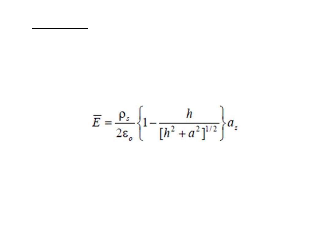
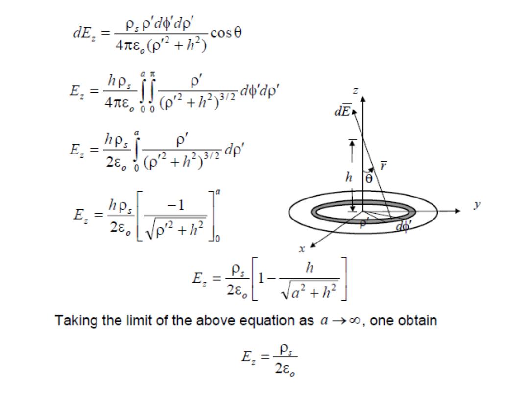
• Example: A circular disk of radius a is
uniformly charged with ρ
s
C /m2. If the disk
lies on the z = 0 plane with its axis along the z
axis,
(a) show that at the point ( 0,0, h )
(b) find the E-field due to an infinite sheet
of charge ρs C /m2 .
35
36
2.6 Field From A Volume Charge Distribution
• If we now visualize a region of space filled with
a tremendous number of charges separated by
minute distances, we see that we can replace
this distribution of very small particles with a
smooth continuous distribution described by a
volume charge density, just as we describe
water as having a density of 1 g/cm3.
• We denote volume charge density by ρν, having
the units of coulombs per cubic meter (C/m3).
37
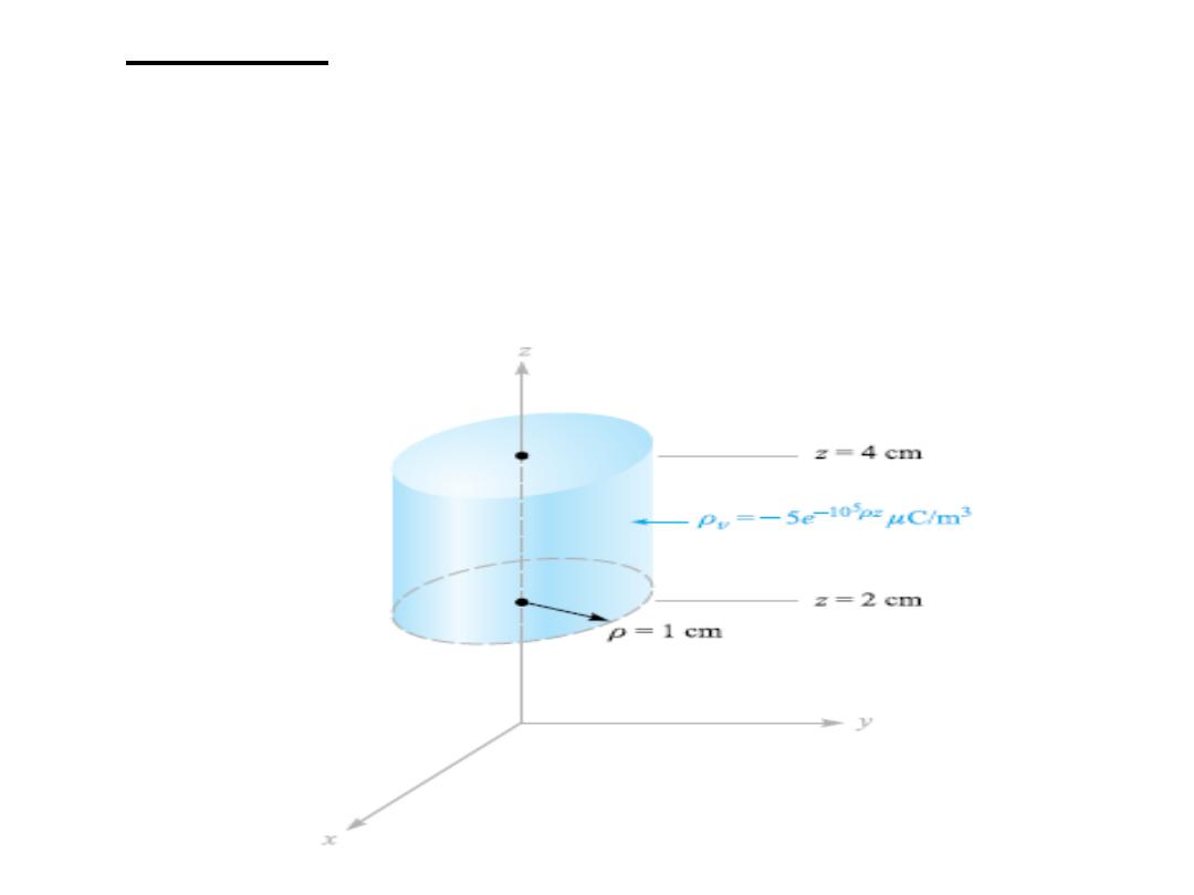
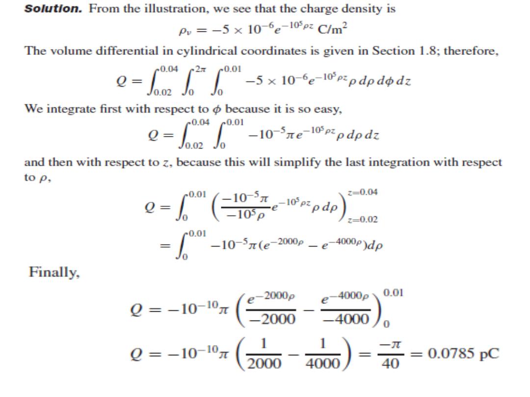
• Example: As an example of the evaluation of a
volume integral, we find the total charge
contained in a 2-cm length of the electron
beam shown in the figure.
38
39