Signals and Systems pdf - م.د منال كاظم عودة

Subjec: Signals and Systems
Lecture 2

Lecture: Dr.Manal Kadhim

Electromechanical Eng.Department
Electromechanical Systems Branch
Fourth Year.

Example one

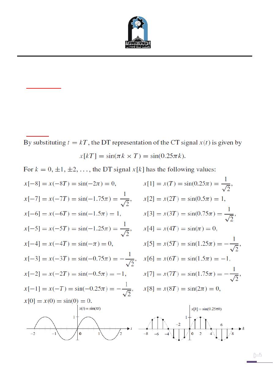
Consider the CT signal x(t ) = sin(πt ) plotted in Fig. 1 (a) as a function of time.

Discretize the signal using a sampling interval of T = 0.25 s, and sketch the

waveform of the resulting DT sequence for the range −8 ≤ k ≤ 8.

Solution

Fig. 1. (a) CT sinusoidal signal (b) DT sinusoidal signal x [k]

Subjec: Signals and Systems
Lecture 2

Lecture: Dr.Manal Kadhim

Electromechanical Eng.Department
Electromechanical Systems Branch
Fourth Year.

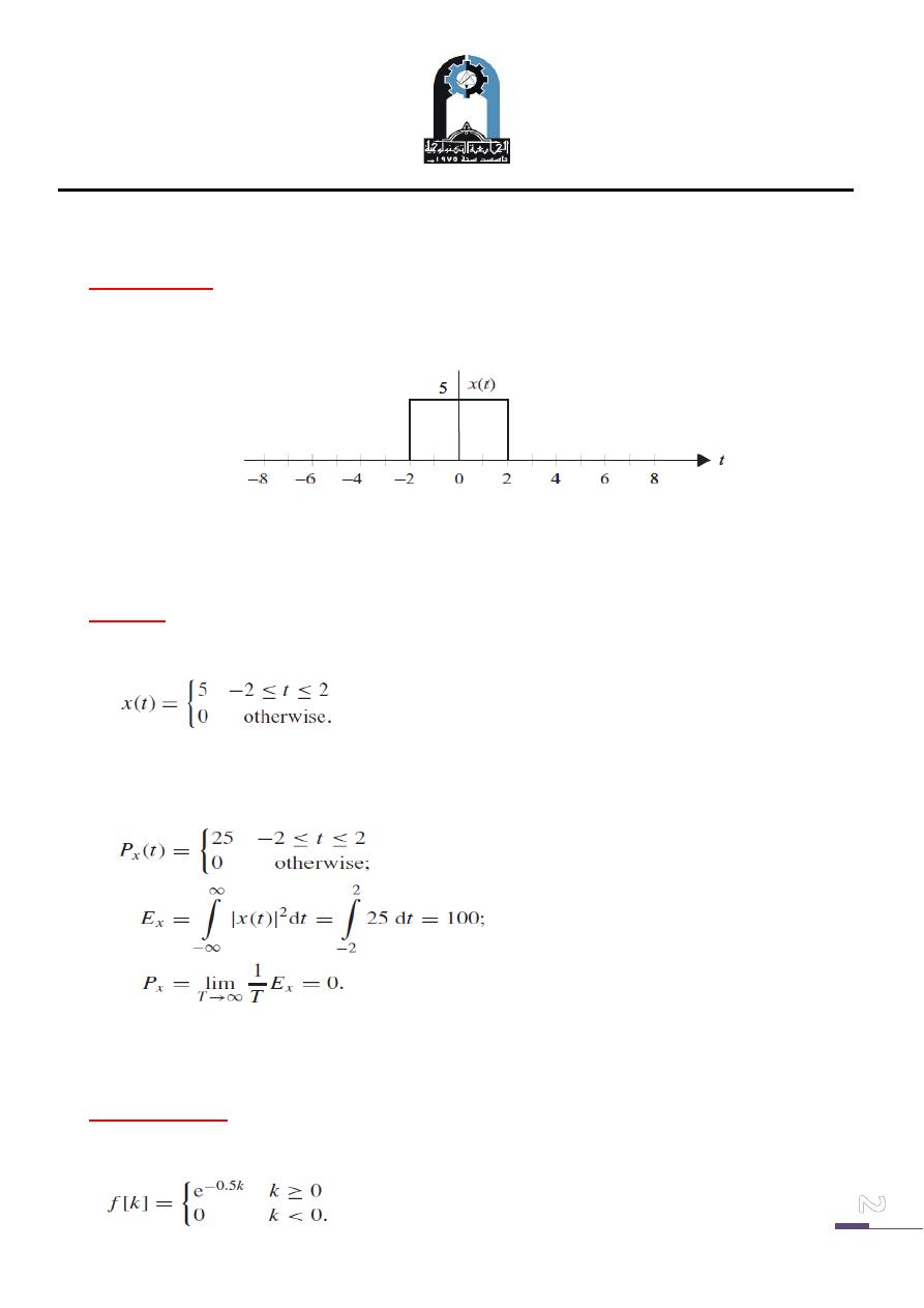
Example Two

Consider the CT signals shown in Figure (2). Calculate the instantaneous power,

average power, and energy of signal. Classify this signals as power or energy signals.

Figure (2)

Solution

The signal x(t ) can be expressed as follows:

The instantaneous power, average power, and energy of the signal are calculated as

follows:

Because x(t ) has finite energy (0 < Ex = 100 < ∞) it is an energy signal.

Example Three

Consider the following DT sequence:

Subjec: Signals and Systems
Lecture 2

Lecture: Dr.Manal Kadhim

Electromechanical Eng.Department
Electromechanical Systems Branch
Fourth Year.

Determine if the signal is a power or an energy signal.

Solution

The total energy of the DT sequence is calculated as follows:

Because Ef is finite, the DT sequence f [k] is an energy signal.

In computing E f , we make use of the geometric progression (GP) series to calculate

the summation.

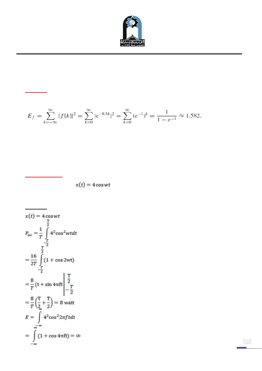
Example Four

Classify the signal

as a power signal or energy signal and find its

power or energy.

Solution

Subjec: Signals and Systems
Lecture 2

Lecture: Dr.Manal Kadhim

Electromechanical Eng.Department
Electromechanical Systems Branch
Fourth Year.

The signal is power signal.

Example Five

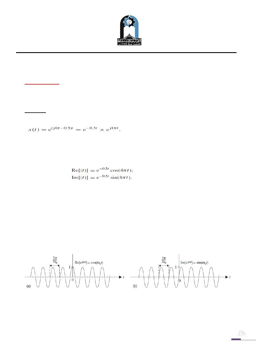
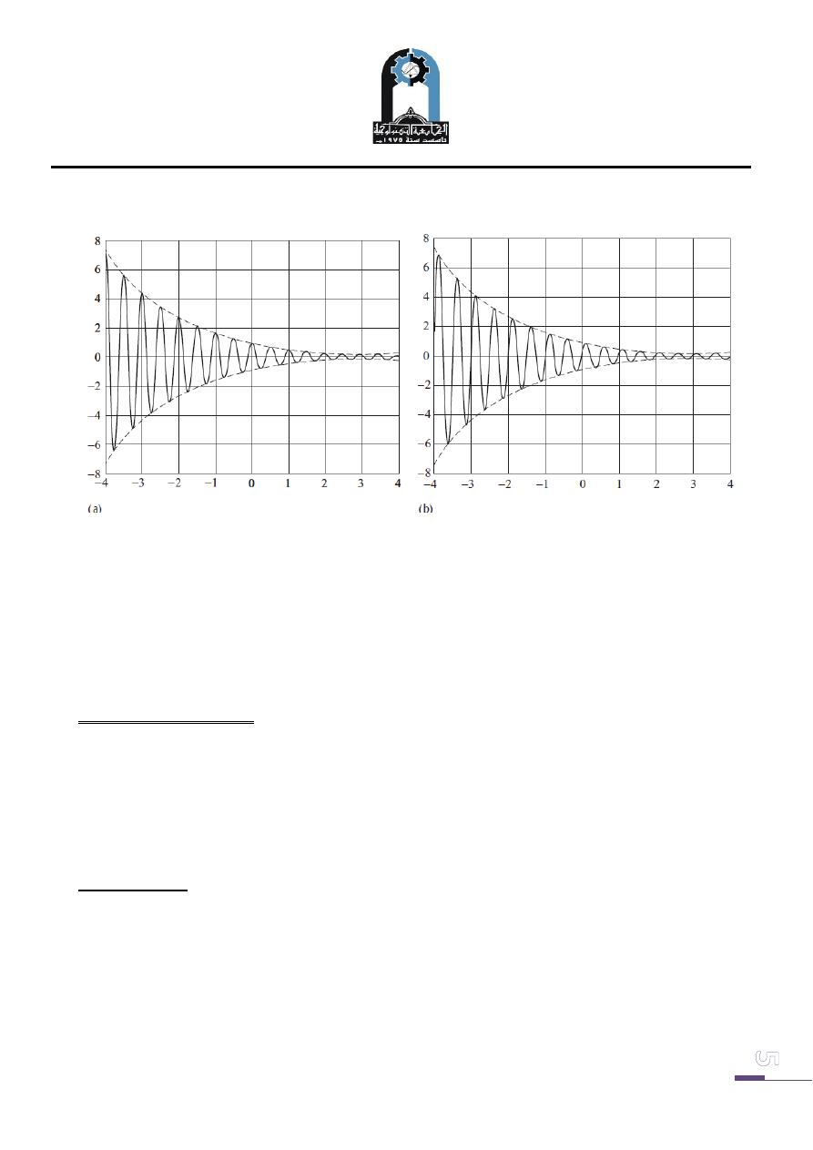
Plot the real and imaginary components of the exponential function x(t ) = exp[(j4π − 0.5)t ] for

−4 ≤ t ≤ 4.

Solution

The CT exponential function is expressed as follows:

The real and imaginary components of x(t ) are expressed as follows:

To plot the real component, we multiply the waveform of a cosine function with

ω0 = 4π, as shown in Fig. 3 (a), by a decaying exponential exp(−0.5t ).

The resulting plot is shown in Fig. 4 (a). Similarly, the imaginary component is

plotted by multiplying the waveform of a sine function with ω0 = 4π, as shown in

Fig. 3 (b), by a decaying exponential exp(−0.5t ). The resulting plot is shown in Fig.

4 (b).

Fig.(3):CT complex-valued exponential function x(t ) = exp( jω0t ).

(a) Real component; (b) imaginary component.

Subjec: Signals and Systems
Lecture 2

Lecture: Dr.Manal Kadhim

Electromechanical Eng.Department
Electromechanical Systems Branch
Fourth Year.

Fig. (4): Exponential function x (t ) = exp[( j4π − 0.5)t ].

(a) Real component; (b) imaginary component.

Signal operations

An important concept in signal and system analysis is the transformation of a signal.

In this section, we consider three elementary transformations that are performed on a

signal in the time domain. The transformations that we consider are time shifting,

time scaling, and time inversion.

Time shifting

The time-shifting operation delays or advances forward the input signal in time.

Consider a CT signal φ(t ) obtained by shifting another signal x(t) by T time units.

The time-shifted signal φ(t ) is expressed as follows:

φ(t) = x(t + T).

In other words, a signal time-shifted by T is obtained by substituting t in x(t) by

Subjec: Signals and Systems
Lecture 2

Lecture: Dr.Manal Kadhim

Electromechanical Eng.Department
Electromechanical Systems Branch
Fourth Year.

(t + T ). If T < 0, then the signal x(t ) is delayed in the time domain. Graphically this

is equivalent to shifting the origin of the signal x(t ) towards the right-hand side by

duration T along the t-axis. If T > 0, then the signal x(t ) is advanced forward in time.

The plot of the time-advanced signal is obtained by shifting x(t ) towards the left-

hand side by duration T along the t-axis.

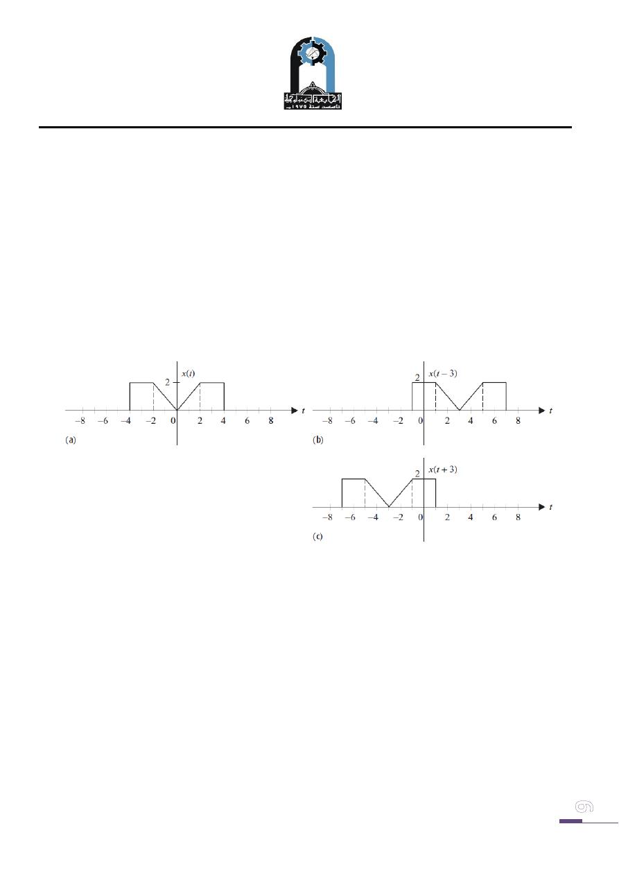
Figure 5(a) shows a CT signal x(t) and the corresponding two time-shifted signals

x(t − 3) and x(t + 3).

Fig. (5): Time shifting of a CTsignal. (a) Original CT signal x(t ).

(b) Time-delayed versionx(t − 3) and (c) Time-advanced versionx(t + 3)

The theory of the CT time-shifting operation can also be extended to DT sequences.

When a DT signal x[k] is shifted by m time units, the delayed signal φ[k] is expressed

as follows:

φ[k] = x[k + m].

If m < 0, the signal is said to be delayed in time. To obtain the time-delayed signal

φ[k], the origin of the signal x[k] is shifted towards the right-hand side along the k-

axis by m time units. On the other hand, if m > 0, the signal is advanced forward in

Subjec: Signals and Systems
Lecture 2

Lecture: Dr.Manal Kadhim

Electromechanical Eng.Department
Electromechanical Systems Branch
Fourth Year.

time. The time-advanced signal φ[k] is obtained by shifting x[k] towards the left-hand

side along the k-axis by m time units.

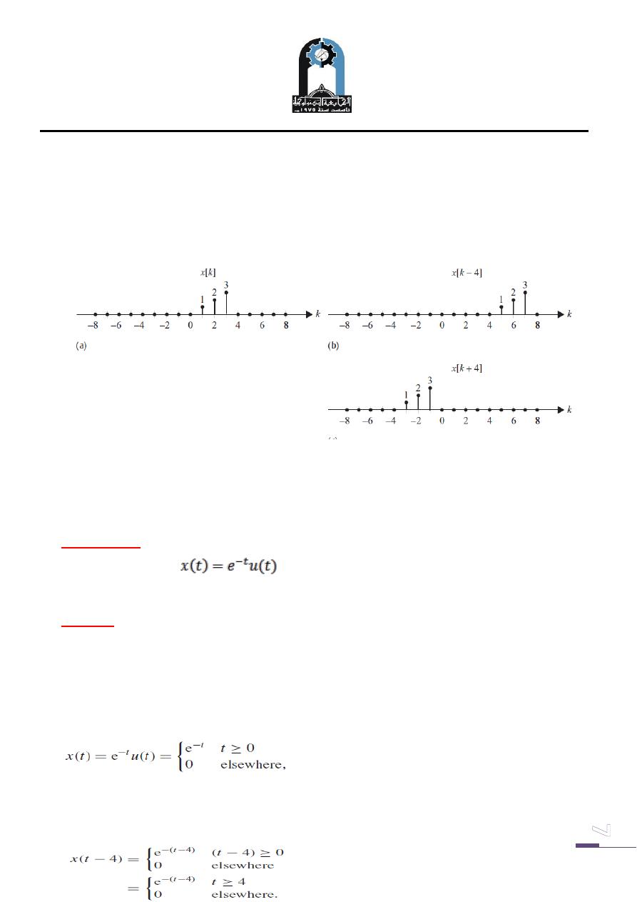
Figure (6) shows a DT signal x[k] and the corresponding two time-shifted signals

x[k − 4] and x[k + 4].

Fig. (6): Time shifting of a DT signal. (a) Original DT signal x[k].

(b) Time-delayed version x[k − 4](c) Time-advanced version x[k + 4]

Example Six

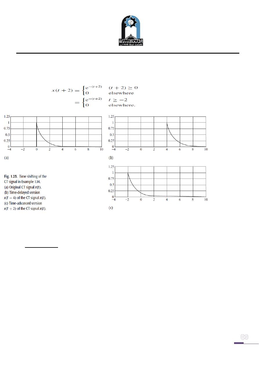
Consider the signal

. Determine and plot the time-shifted versions

x(t − 4) and x(t + 2).

Solution

The signal x(t ) can be expressed as follows:

and is shown in Fig. 7(a). To determine the expression for x(t − 4), we substitute t by

(t − 4). The resulting expression is given by the function x(t − 4) is plotted in Fig.

Subjec: Signals and Systems
Lecture 2

Lecture: Dr.Manal Kadhim

Electromechanical Eng.Department
Electromechanical Systems Branch
Fourth Year.

7(b). Similarly, we can calculate the expression for x(t + 2) by substituting t by(t + 2)

in. The resulting expression is given by

Fig. (7):

Time

shifting

of the CT

signal (a)

Original

signal x(t

). (b)

Time-

delayed

version

x(t − 4) of the CT signal x(t ).(c) Time-advanced version x(t + 2) of the CT signal x(t ).

Time scaling

The time-scaling operation compresses or expands the input signal in the time

domain. A CT signal x(t) scaled by a factor c in the time domain is denoted by x(ct).

If c > 1, the signal is compressed by a factor of c. On the other hand, if 0 < c < 1 the

signal is expanded.

Subjec: Signals and Systems
Lecture 2

Lecture: Dr.Manal Kadhim

Electromechanical Eng.Department
Electromechanical Systems Branch
Fourth Year.

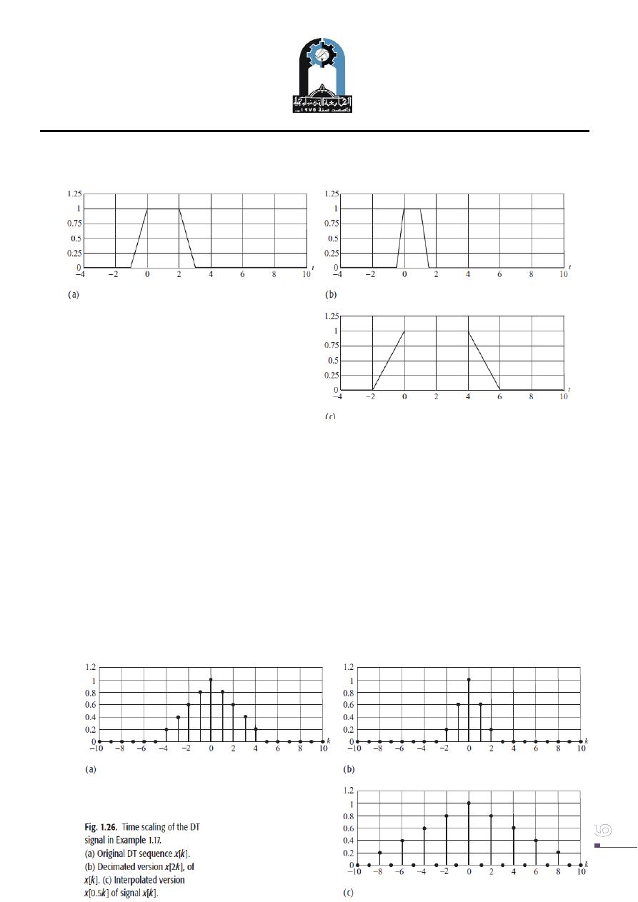
Fig.(8) : Example of Time scaling of the CT signal

(a) Original CT signal x(t ).(b) Time-compressed version x(2t) of x(t ).

(c) Time-expanded version x(0.5t ) of signal x(t ).

The time scaling of the DT sequence in the following.

Decimation: If a sequence x[k] is compressed by a factor c, some data samples of

x[k] are lost. For example, if we decimate x[k] by 2, the decimated function y[k]

=x[2k] retains only the alternate samples given by x[0], x[2], x[4].

Subjec: Signals and Systems
Lecture 2

Lecture: Dr.Manal Kadhim

Electromechanical Eng.Department
Electromechanical Systems Branch
Fourth Year.

Time inversion

The time inversion (also known as time reversal or reflection) operation reflects the

input signal about the vertical axis (t = 0). When a CT signal x(t) is time reversed, the

inverted signal is denoted by x(−t). Likewise, when a DT signal x[k] is time-reversed,

the inverted signal is denoted by x[−k].

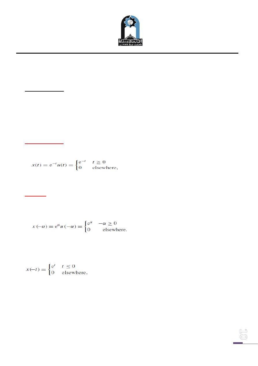
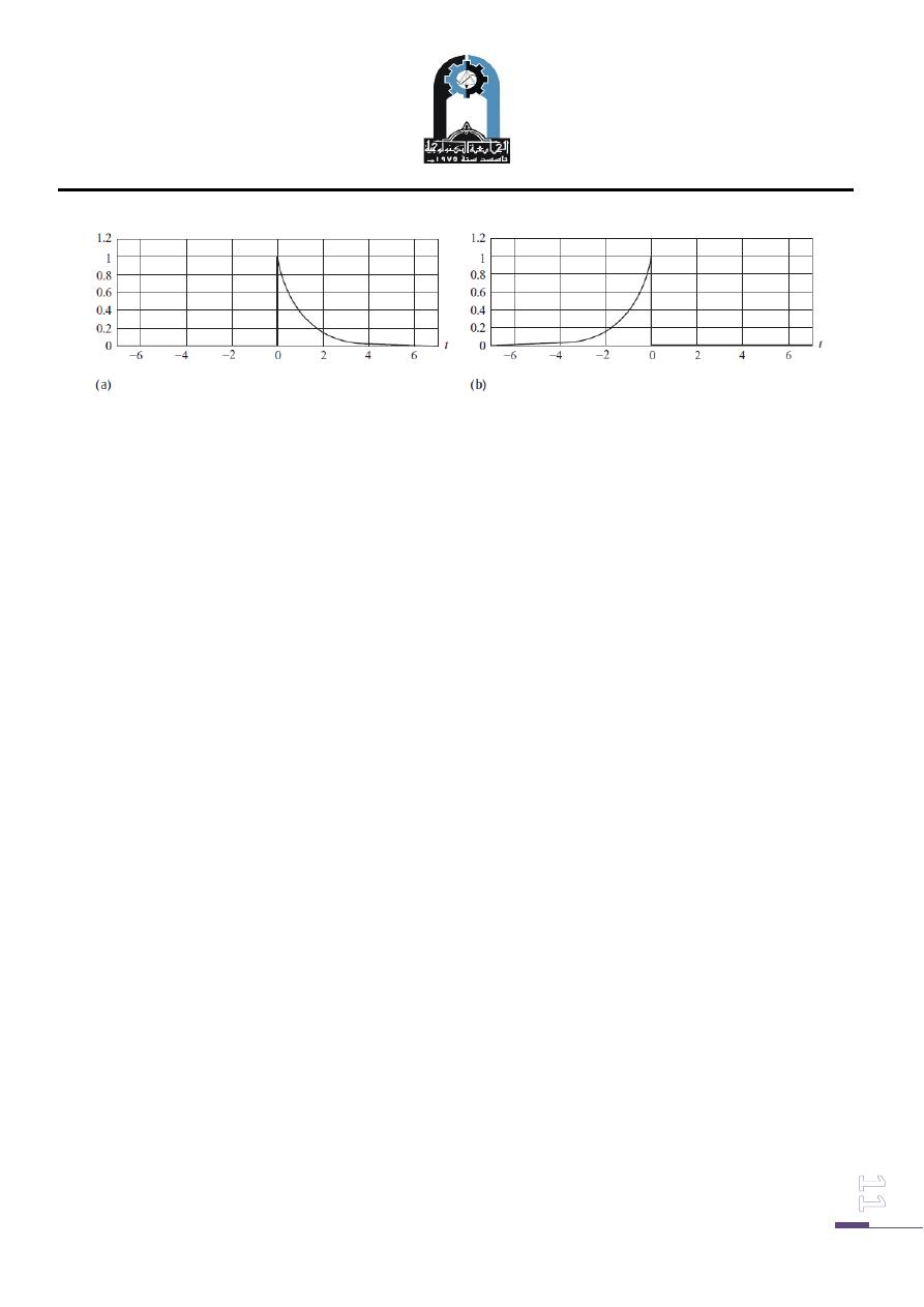
Example Seven

Sketch the time-inverted version of the causal decaying exponential signal

which is plotted in Fig. 10(a).

Solution

To derive the expression for the time-inverted signal x(−t ), substitute t = −α. The

resulting expression is given by

Simplifying the above expression and expressing it in terms of the independent

variable t yields

)

Subjec: Signals and Systems
Lecture 2

Lecture: Dr.Manal Kadhim

Electromechanical Eng.Department
Electromechanical Systems Branch
Fourth Year.

Fig. (10): Time inversion of the CT signal (a) Original CT signal x(t ).

(b) Time-inverted version x(−t ).

Subjec: Signals and Systems
Lecture 2

Lecture: Dr.Manal Kadhim

Electromechanical Eng.Department
Electromechanical Systems Branch
Fourth Year.

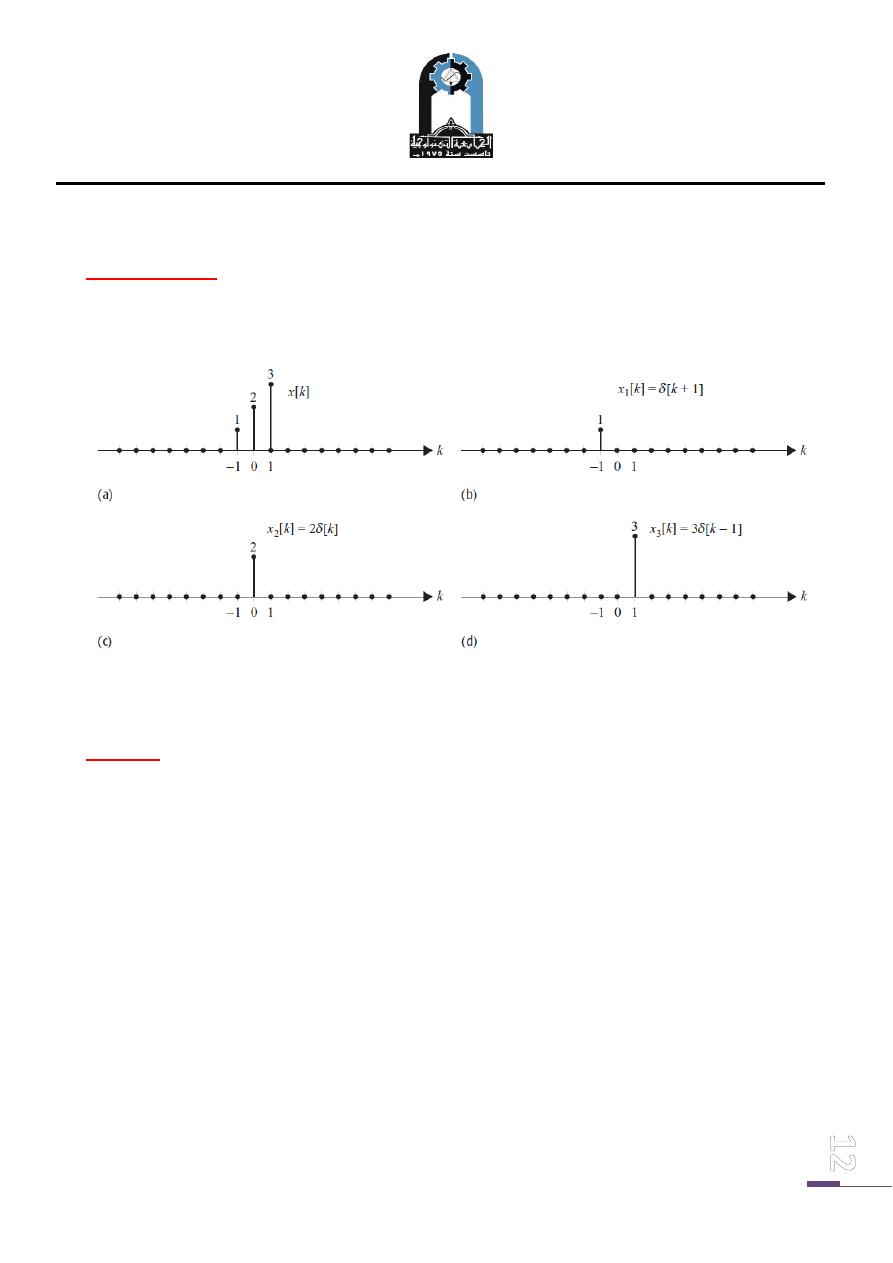
Example Eight

Represent the DT sequence shown in Fig. 11(a) as a function of time-shifted DT unit

impulse functions.

fig.(11): The DT function in (a) is the sum of the shifted

DT impulse functions shown in (b), (c), and (d).

Solution

The DT signal x[k] can be represented as the summation of three functions, x1[k],

x2[k], and x3[k], as follows:

x[k] = x1[k] + x2[k] + x3[k],

where x1[k], x2[k], and x3[k] are time-shifted impulse functions,

x1[k] = δ[k + 1], x2[k] = 2δ[k], and x3[k] = 3δ[k − 1],

and are plotted in Figs. 1. (b), (c), and (d), respectively. The DT sequence x[k] can

therefore be represented as follows:

x[k] = δ[k + 1] + 2δ[k] + 3δ[k − 1].