
Subjec: Signals and Systems
Lecture 1
Lecture: Dr.Manal Kadhim
Electromechanical Eng.Department
Electromechanical Systems Branch
Fourth Year.
I
I
n
n
t
t
r
r
o
o
d
d
u
u
c
c
t
t
i
i
o
o
n
n
t
t
o
o
S
S
i
i
g
g
n
n
a
a
l
l
s
s
a
a
n
n
d
d
S
S
y
y
s
s
t
t
e
e
m
m
s
s
What are Signals?
Signals are detectable quantities used to convey information about time-varying
physical phenomena. Common examples of signals are human speech, temperature
and pressure. Electrical signals, normally expressed in the form of voltage or current
waveforms, are some of the easiest signals to generate and process.
Mathematically, signals are modeled as functions of one or more independent
variables. Examples of independent variables used to represent signals are time,
frequency.
What are systems?
A system is an interconnection of components that transforms an input signal
into an output signal. It is establishes a relationship between a set of inputs and the
corresponding set of outputs.
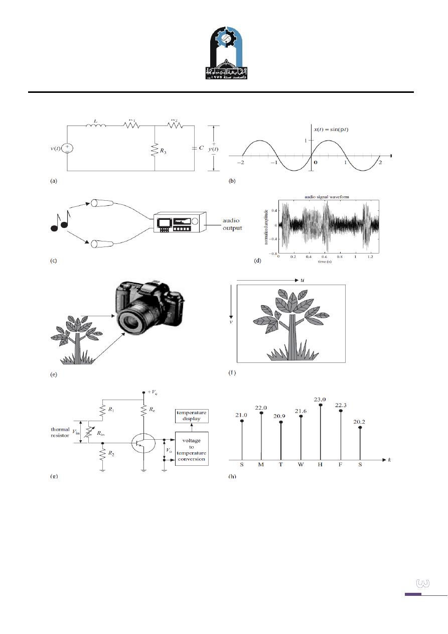
Figure (1) illustrates some common signals and systems encountered in different
fields of engineering.
Figure (1a) is a simple electrical circuit consisting of three passive components. A
voltage v(t) is applied at the input of the RLC circuit, which produces an output
voltage y(t) across the capacitor. A possible waveform for y(t) is the sinusoidal signal
shown in Fig. (1b). Figure (1. c) shows an audio recording system where the input
signal is an audio or a speech waveform. The function of the audio recording system
is to convert the audio signal into an electrical waveform, which is recorded on a
magnetic tape or a compact disc. A possible resulting waveform for the recorded
electrical signal is shown in Fig. (1 d). Figure (1. e) shows a charge coupled device
(CCD) based digital camera where the input signal is the light emitted from a scene.

Subjec: Signals and Systems
Lecture 1
Lecture: Dr.Manal Kadhim
Electromechanical Eng.Department
Electromechanical Systems Branch
Fourth Year.
The incident light charges a CCD panel located inside the camera, thereby storing the
external scene in terms of the spatial variations of the charges on the CCD panel.
Figure (1g) illustrates a thermometer that measures the ambient
temperature of its environment. Electronic thermometers typically use a thermal
resistor, known as a thermistor, whose resistance varies with temperature. The
fluctuations in the resistance are used to measure the temperature. Figure (1h).
Subjec: Signals and Systems
Lecture 1
Lecture: Dr.Manal Kadhim
Electromechanical Eng.Department
Electromechanical Systems Branch
Fourth Year.
Fig. (1) Examples of signals and systems. (a) An electrical circuit; (c) an audio recording
system; (e) adigital camera; and (g) a digital thermometer. Plots (b), (d), (f ), and (h) are
output signals generated,respectively, by the systems shown in (a), (c), (e), and (g).
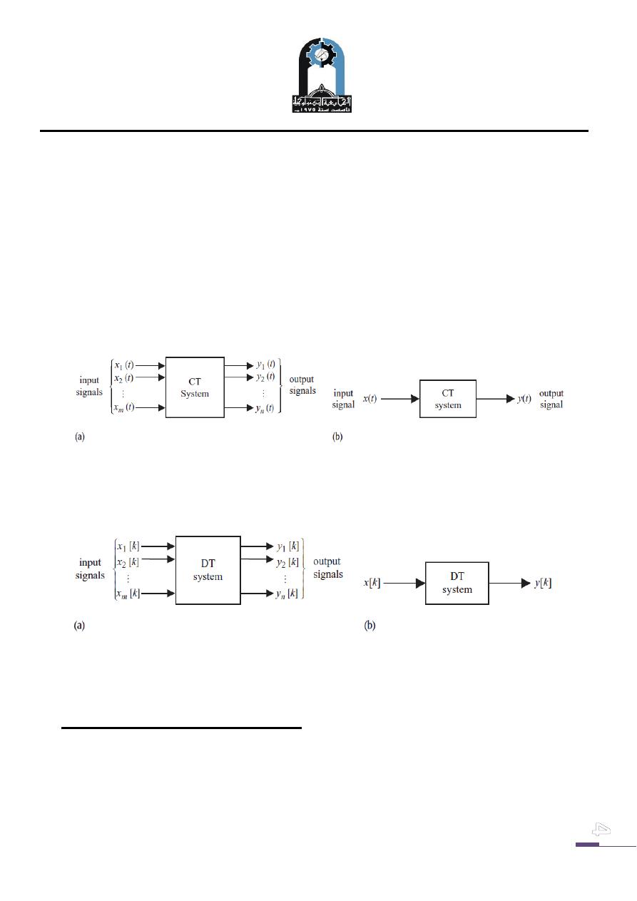
Most physical processes are modeled by multiple-input and multiple-output (MIMO)
systems of the form illustrated in Fig. (2a) where the xi (t)’s represent the continuous
Subjec: Signals and Systems
Lecture 1
Lecture: Dr.Manal Kadhim
Electromechanical Eng.Department
Electromechanical Systems Branch
Fourth Year.
time inputs while the yj (t)’s represent the continuous time outputs, or single-input,
single-output illustrated in Fig. (2.b) . Such systems, which operate on continuous
time input signals transforming them to continuous time output signals are referred to
as continuous time systems.
In comparison to continuous time systems, discrete time systems transform discrete
time input signals, often referred to as sequences, into discrete time output signals.
two discrete time systems are shown in Fig. (3.a) and Fig. (3b).
Fig. (2):
Continuous Time systems. (a) Multiple-input, multiple-output (MIMO)
(b) Single-input, single-output CT system.
Fig. (3): Discrete Time systems. (a) Multiple-input,multiple-output (MIMO) DT system
. (b) Single-input,single-output DT system.
.
Why study Signals and Systems?
Signals and systems are fundamental to all of engineering.
The aims of signals and system course are :
To represent and manipulate signals.
To represent and characterize systems.
Subjec: Signals and Systems
Lecture 1
Lecture: Dr.Manal Kadhim
Electromechanical Eng.Department
Electromechanical Systems Branch
Fourth Year.
To understand the effect of standard signals on liner system.
Classification of Signals
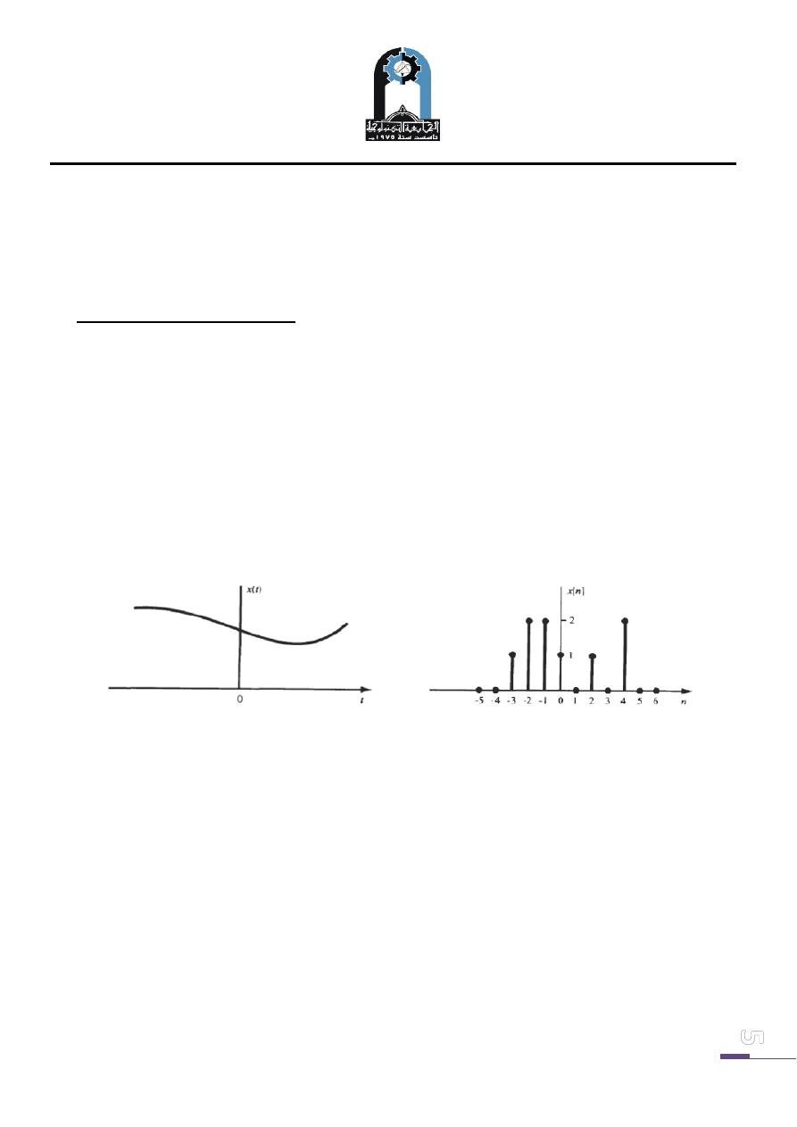
A. Continuous-Time and Discrete-Time Signals:
A signal x(t) is a continuous-time signal if t is a continuous variable. If t is a discrete
variable that is, x(t) is defined at discrete times, then x(t) is a discrete-time signal.
Since a discrete-time signal is defined at discrete times, a discrete-time signal is often
identified as a sequence of numbers, denoted by {x
n
} or x[n], where n=integer.
Illustrations of a continuous-time signal x(t) and of a discrete-time signal x[n] are
shown in Figure below.
Continuous-time signal discrete-time signal
A discrete-time signal x[n] may be obtained by sampling a continuous-time signal
x(t). Many physical systems operate in continuous time, Digital computations are
done in discrete time
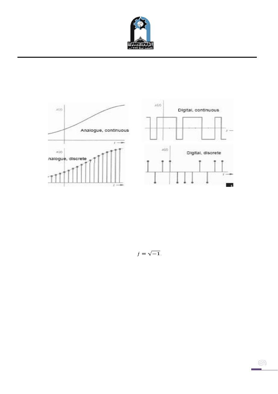
B. Analog and Digital Signals:
If a continuous-time signal x(t) can take on any value in the continuous interval (a,
b), where a may be -
∞ and b may be +∞, then the continuous-time signal x(t) is
called an analog signal. If a discrete-time signal x[n] can take on only a finite
Subjec: Signals and Systems
Lecture 1
Lecture: Dr.Manal Kadhim
Electromechanical Eng.Department
Electromechanical Systems Branch
Fourth Year.
number of distinct values, then we call this signal a digital signal. Figure below show
examples big analogue and digital signals.
C. Real and Complex Signals:
A signal x(t) is a real signal if its value is a real number, and a signal x(t) is a
complex signal if its value is a complex number. A general complex signal x(t) a
function of the form
x (t) = x
1
(t) + jx
2
(t)
where x
1
(t) and x
2
(t) are real signals and
.
D. Deterministic and Random Signals:
Deterministic signals are those signals whose values are specified for any given time.
Thus, a deterministic signal can be modeled by a known function of time t.(
modeled
by clear mathematical express
ions , such as χ ( t) =A coswt).
Subjec: Signals and Systems
Lecture 1
Lecture: Dr.Manal Kadhim
Electromechanical Eng.Department
Electromechanical Systems Branch
Fourth Year.
Random
s
ignals are those signals that take random values at any given time (it is not
possible to write clear mathematical expressions), and must be characterized
statistically.
Deterministic signal Random signal
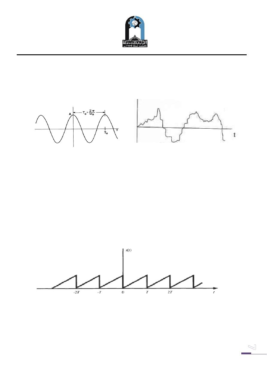
E. Periodic and Nonperiodic Signals:
A continuous-time signal x (t) is said to be periodic with period T if
x(t +T) = x (t) for all t
An example of such a signal is given in Fig. below. From Fig. it follows that
x(t +mT) = x (t) for all t and any integer m.
The fundamental period T
0
, of x (t) is the smallest positive value of T.
Examples of continuous-time periodic signals
Any continuous-time signal which is not periodic is called a nonperiodic (or a
periodic) signal.
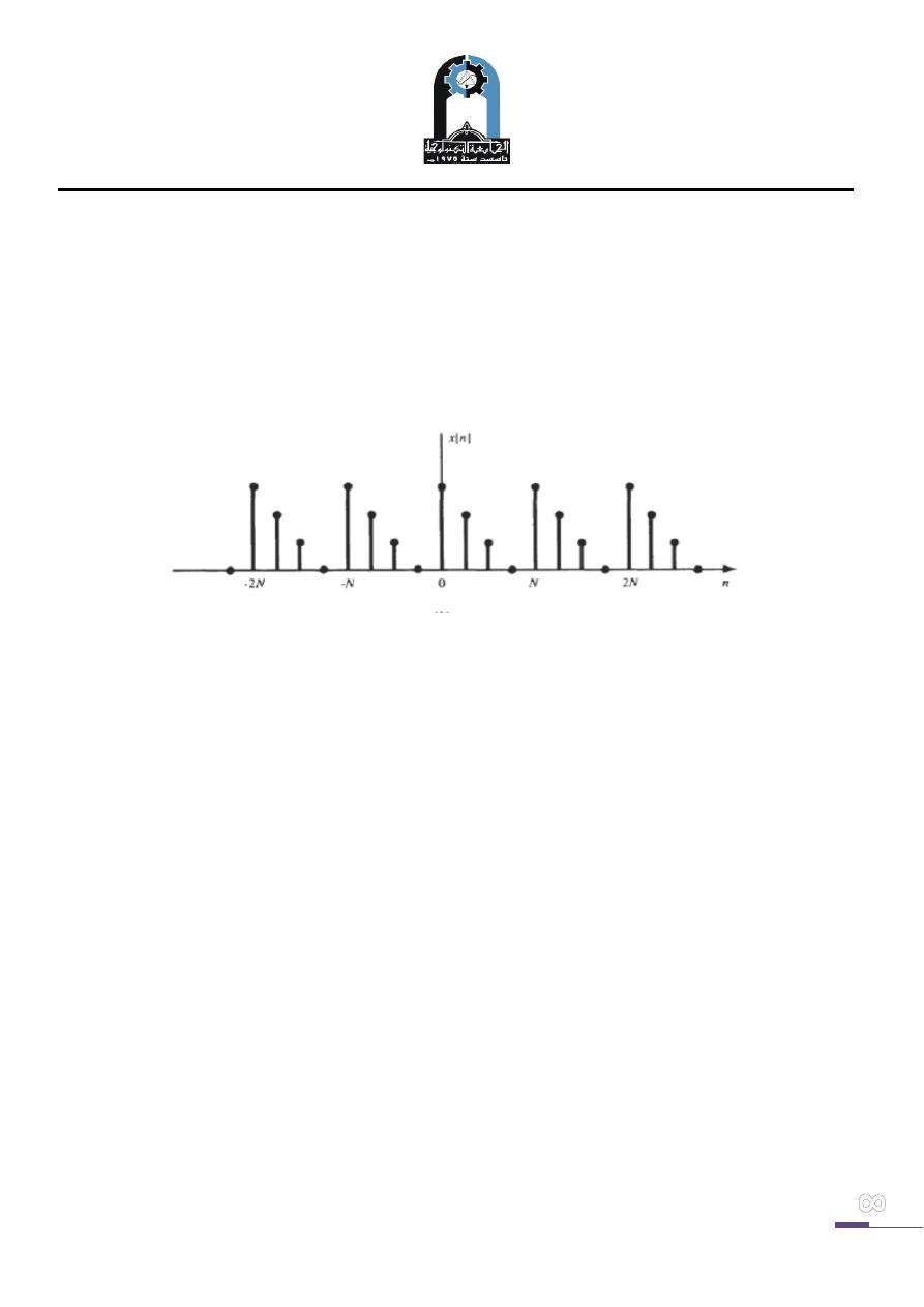
A sequence (discrete-time signal) x[n] is periodic with period N if there is a positive
integer N for which
x ( t )
x ( t )
Subjec: Signals and Systems
Lecture 1
Lecture: Dr.Manal Kadhim
Electromechanical Eng.Department
Electromechanical Systems Branch
Fourth Year.
x[n +N] =x[n] for all n
An example of such a sequence is given in Fig. bellow. From Fig. it follows that
x[n+mN] =x[n] for all n and any integer m.
The fundamental period N
0
of x[n] is the smallest positive integer N.
Examples of discrete-time periodic signals
Any sequence which is not periodic is called a nonperiodic (or a periodic) sequence.
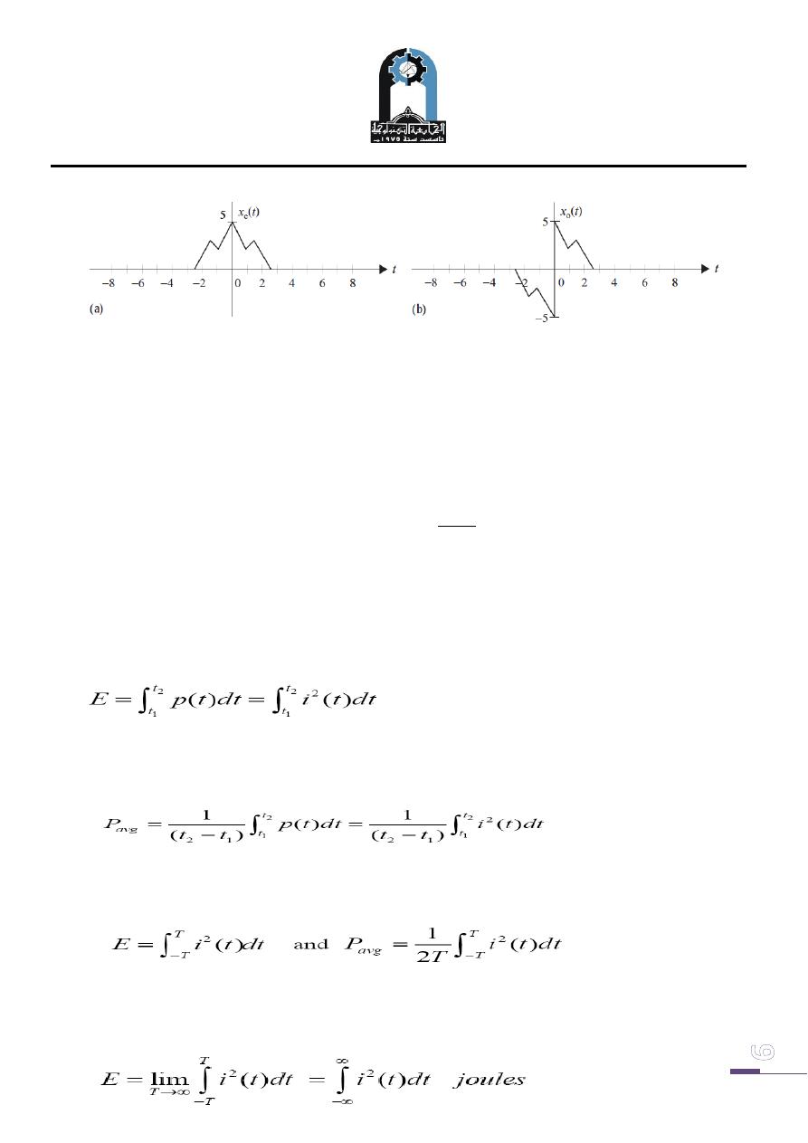
F. Even and Odd Signals:
A signal x ( t ) or x[n] is referred to as an even signal if
x(-t) = x(t)
x[-n] = x[n]
A signal x (t) or x[n] is referred to as an odd signal if
x(-t) = - x(t)
x[-n] = - x[n]
Examples of even and odd signals are shown in Fig.
Subjec: Signals and Systems
Lecture 1
Lecture: Dr.Manal Kadhim
Electromechanical Eng.Department
Electromechanical Systems Branch
Fourth Year.
(a) even signals (b) odd signals
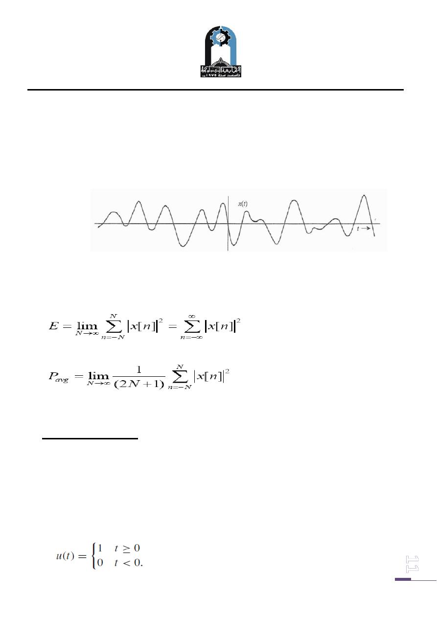
G. Energy and Power Signals:
Consider e(t) to be the voltage across a resistor R producing a current i(t). The
instantaneous power p(t) per ohm is defined as:
R
t
i
R
t
v
t
i
t
v
t
p
)
(
)
(
)
(
)
(
)
(
Since power is the rate of energy, the total energy expended over the time interval
2
1
t
t
t
is :
and the average power over this interval is:
If t
1
= -T and t
2
= T then,
If i(t) is a continuous-time signal, the total energy E and average power P on a per-
ohm basis are
Subjec: Signals and Systems
Lecture 1
Lecture: Dr.Manal Kadhim
Electromechanical Eng.Department
Electromechanical Systems Branch
Fourth Year.
and
For an arbitrary continuous-time signal x(t), the total energy normalized to unit
resistance is defined as
and the average power normalized to unit resistance is defined as
Based on the above definition, the following classes of signals are defined:
1) x(t) is an energy signal if and only if 0<E<
∞
(having finite energy), so that
P=0.
2) x(t) is a power signal if and only if 0<P<
∞, thus implying that E=∞.
3) Signals that satisfy neither property are therefore neither energy nor power
signals.
An energy signal has zero average power, whereas a power signal has infinite energy.
Thus the periodic signals are classified as power signals. Figures below shows an
example of energy and power signals.
Subjec: Signals and Systems
Lecture 1
Lecture: Dr.Manal Kadhim
Electromechanical Eng.Department
Electromechanical Systems Branch
Fourth Year.
Energy Signal: Signal with finite energy (zero power)
Power Signal: Signal with finite power (infinite energy)
In discrete time
and
Elementary signals
Representing signals in terms of the elementary functions simplifies the analysis and
design of linear systems.
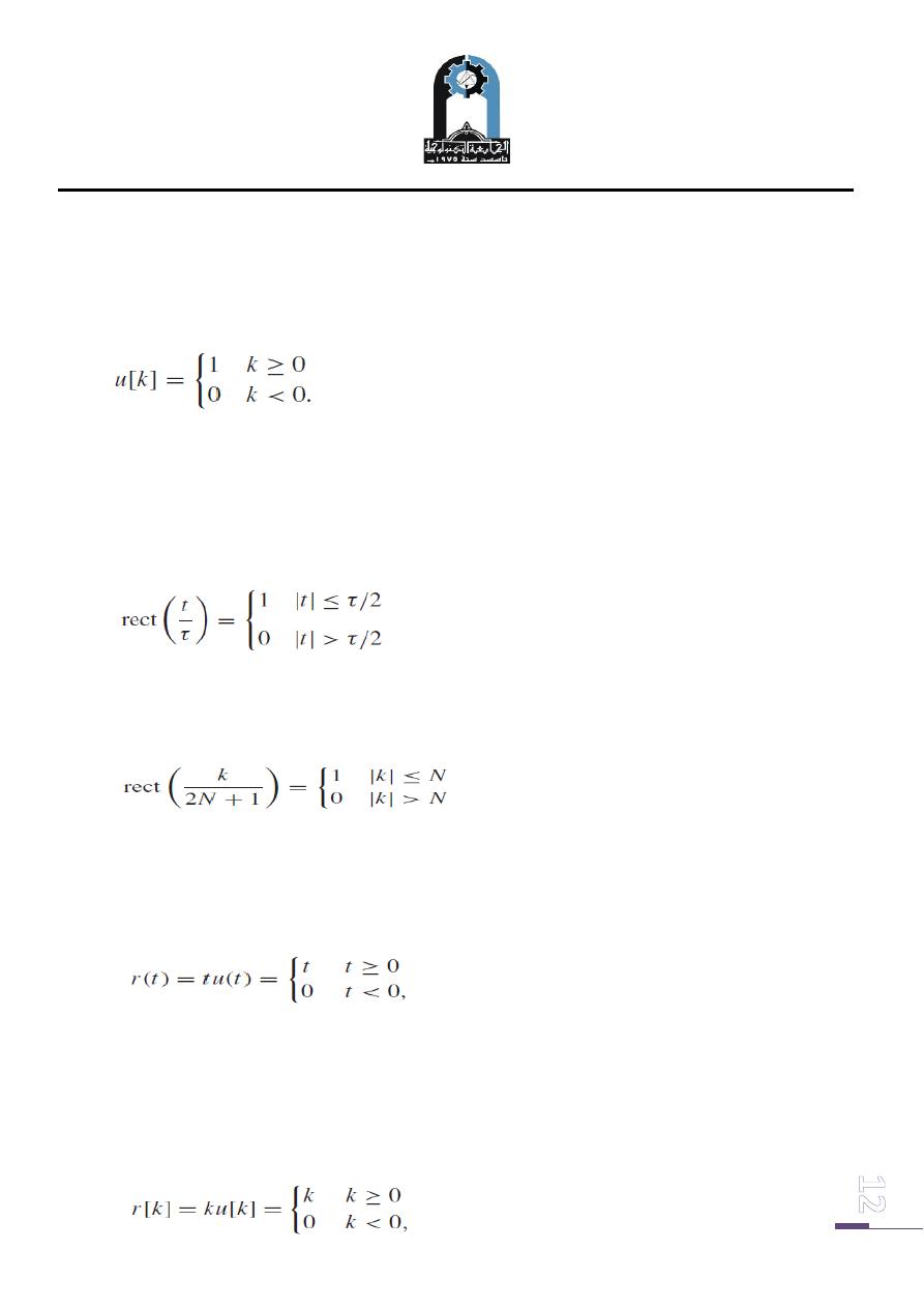
1. Unit step function
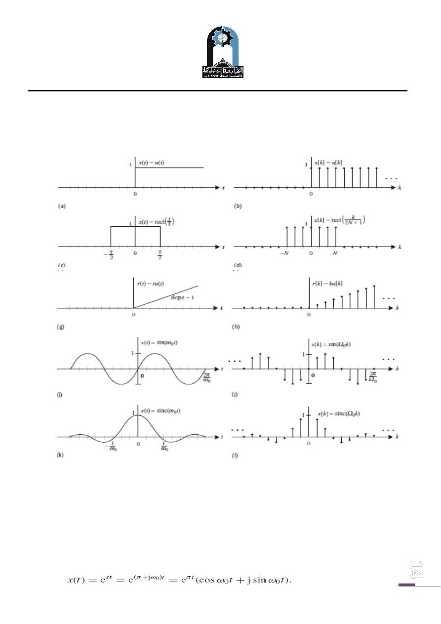
The CT unit step function u(t ) is defined as follows:
Subjec: Signals and Systems
Lecture 1
Lecture: Dr.Manal Kadhim
Electromechanical Eng.Department
Electromechanical Systems Branch
Fourth Year.
The DT unit step function u[k] is defined as follows:
The waveforms for the unit step functions u(t ) and u[k] are shown, respectively, in
Figs.4 (a) and (b).
2. Rectangular pulse function
The CT rectangular pulse rect(t/τ ) is defined as follows:
and it is plotted in Fig. 4(c). The DT rectangular pulse rect(k/(2N + 1)) is
defined as follows:
and it is plotted in Fig. 4(d).
3. Ramp function
The CT ramp function r (t ) is defined as follows:
which is plotted in Fig. 4(g).
Similarly, the DT ramp function r [k] is defined
as follows:
Subjec: Signals and Systems
Lecture 1
Lecture: Dr.Manal Kadhim
Electromechanical Eng.Department
Electromechanical Systems Branch
Fourth Year.
which is plotted in Fig. 4(h).
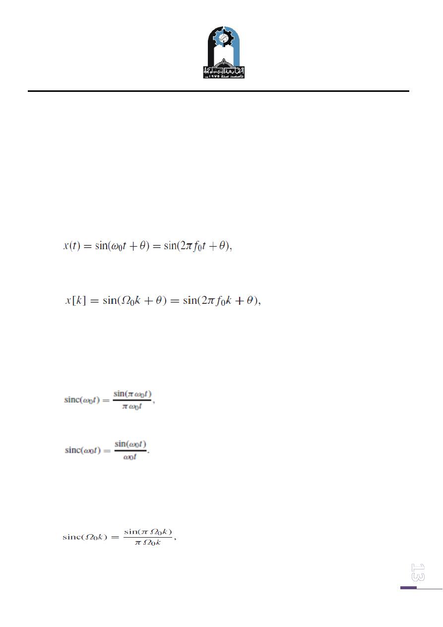
4. Sinusoidal function
The CT sinusoid of frequency f0 (or, equivalently, an angular frequency ω0 =2π f0
is defined as follows:
which is plotted in Fig. 4(i). The DT sinusoid is defined as follows:
where Ω0 is the DT angular frequency. The DT sinusoid is plotted in Fig. 4(j).
5. Sinc function
The CT sinc function is defined as follows:
Or
which is plotted in Fig. 1.12(k)
The DT sinc function is defined as follows:
which is plotted in Fig. 4(l).
Subjec: Signals and Systems
Lecture 1
Lecture: Dr.Manal Kadhim
Electromechanical Eng.Department
Electromechanical Systems Branch
Fourth Year.
Fig.( 4):. CT and DT elementary functions. (a) CT and (b) DT unit step functions. (c) CT and
(d) DT rectangular pulses. (g) CT and (h) DT ramp functions. (i) CT and (j) DT sinusoidal
functions. (k) CT and (l) DT sinc functions.
6. CT exponential function
A CT exponential function, with complex frequency s = σ + jω0, is represented
by
Subjec: Signals and Systems
Lecture 1
Lecture: Dr.Manal Kadhim
Electromechanical Eng.Department
Electromechanical Systems Branch
Fourth Year.
The CT exponential function is, therefore, a complex-valued function with the
following real and imaginary components:
Depending upon the presence or absence of the real and imaginary components,
there are two special cases of the complex exponential function.
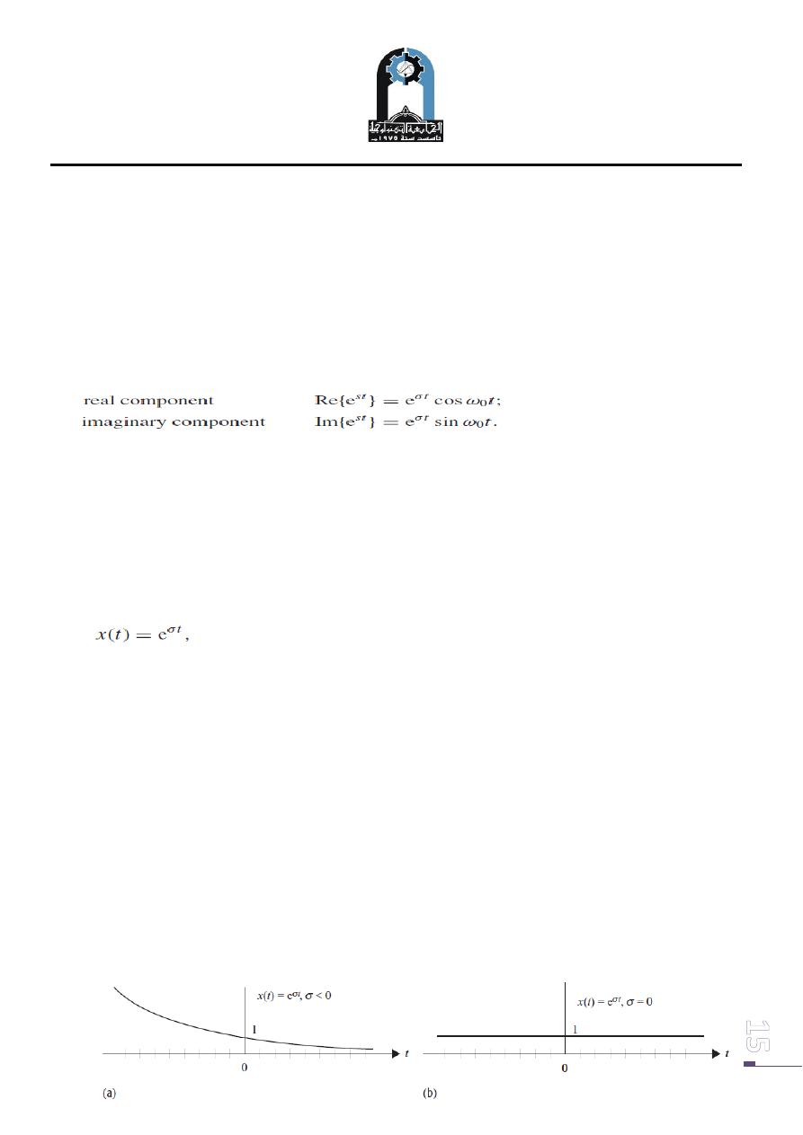
Case 1: Imaginary component is zero (ω0 = 0)
Assuming that the imaginary component ω of the complex frequency s is zero,
the exponential function takes the following form:
which is referred to as a real-valued exponential function. Figure (5) shows the real-
valued exponential functions for different values of σ. When the value of σ is
negative (σ < 0) then the exponential function decays with increasing time t .
The exponential function for σ < 0 is referred to as a decaying exponential function
and is shown in Fig. 5(a). For σ = 0, the exponential function has a constant value, as
shown in Fig. 5(b). For positive values of σ (σ > 0), the exponential function
increases with time t and is referred to as a rising exponential function. The rising
exponential function is shown in Fig. 5(c).
Subjec: Signals and Systems
Lecture 1
Lecture: Dr.Manal Kadhim
Electromechanical Eng.Department
Electromechanical Systems Branch
Fourth Year.
Fig. (5): Special cases of real-valued CT exponential function x(t ) = exp(σt ).
(a) Decaying exponential with σ < 0.
(b) Constant with σ = 0.
(c) Rising exponential withσ > 0
.
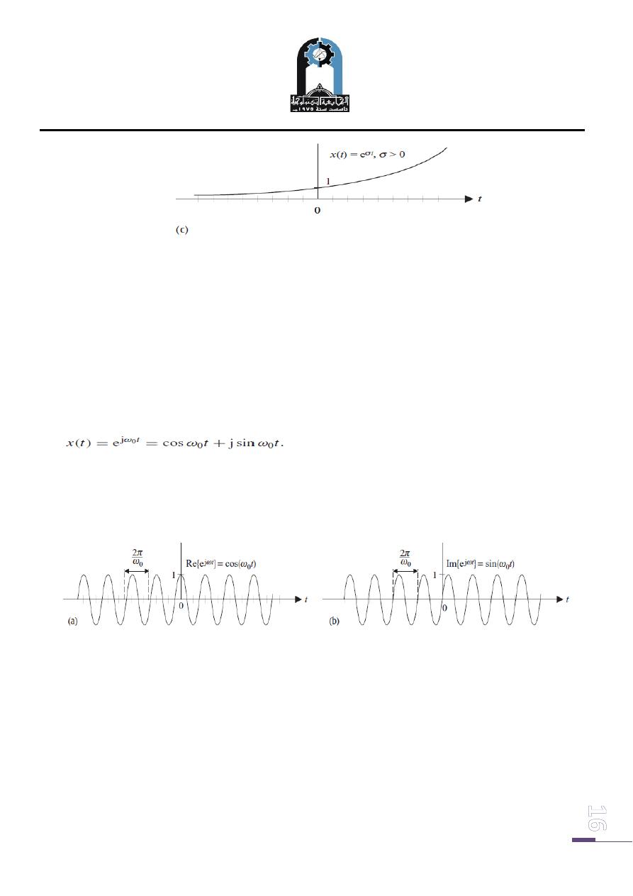
Case 2: Real component is zero (σ = 0)
When the real component σ of the complex frequency s is zero, the exponential
function is represented by
In other words, the real and imaginary parts of the complex exponential are
pure sinusoids. Figure (6) shows the real and imaginary parts of the complex
exponential function
.
Fig. (6): CT complex-valued exponential function x(t ) = exp( jω0t ).
(a) Real component; (b) imaginary component.
Subjec: Signals and Systems
Lecture 1
Lecture: Dr.Manal Kadhim
Electromechanical Eng.Department
Electromechanical Systems Branch
Fourth Year.
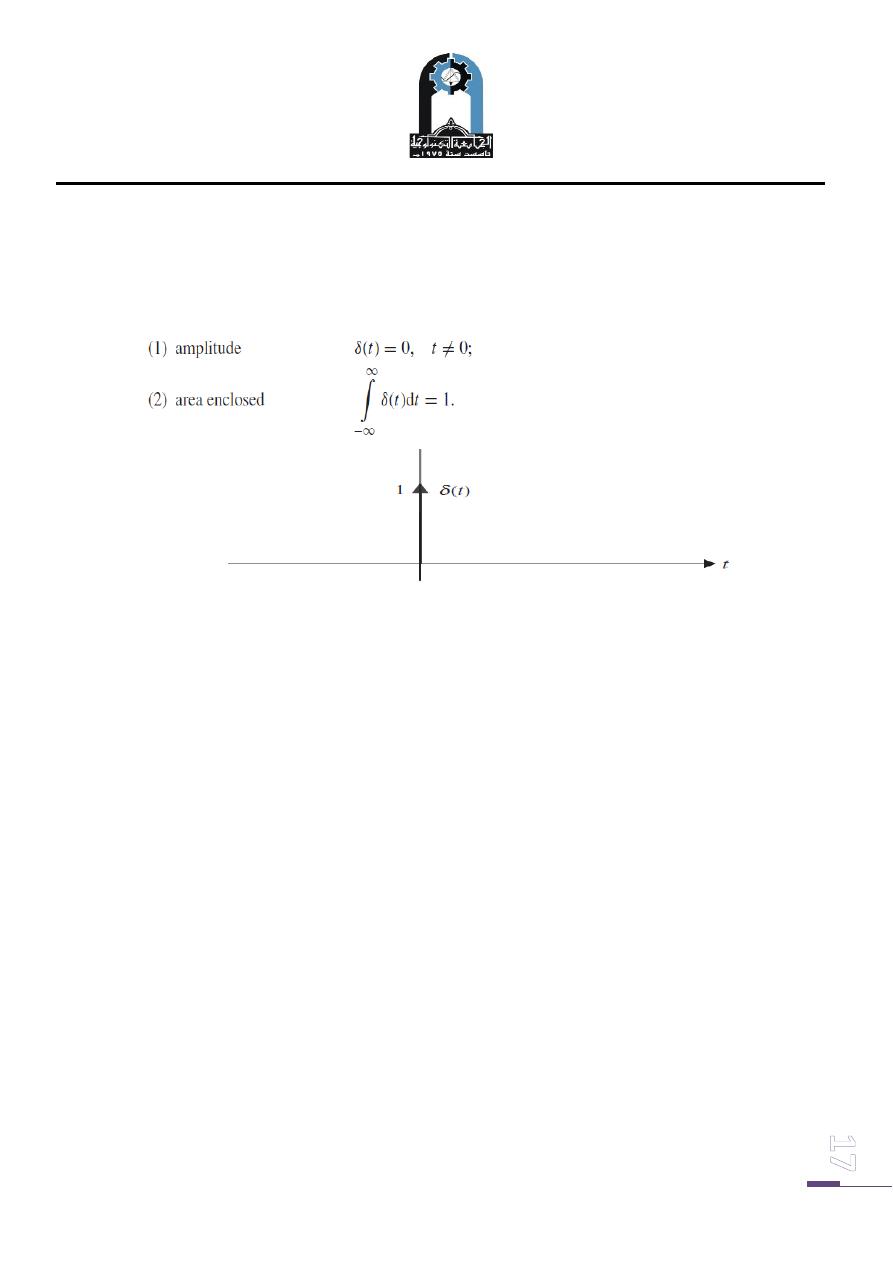
7. CT unit impulse function
The unit impulse function δ(t ), also known as the delta function, is defined in terms
of two properties as follows:
Impluse function