
Signals and Systems
Richard Baraniuk
NONRETURNABLE
NO REFUNDS, EXCHANGES, OR CREDIT ON ANY COURSE PACKETS


Signals and Systems
Course Authors:
Richard Baraniuk
Contributing Authors:
Thanos Antoulas
Richard Baraniuk
Adam Blair
Steven Cox
Benjamin Fite
Roy Ha
Michael Haag
Don Johnson
Ricardo Radaelli-Sanchez
Justin Romberg
Phil Schniter
Melissa Selik
John Slavinsky
Michael Wakin

Produced by:
The Connexions Project
http://cnx.rice.edu/
Rice University, Houston TX
Problems? Typos? Suggestions? etc...
http://mountainbunker.org/bugReport
c
2003 Thanos Antoulas, Richard Baraniuk, Adam Blair, Steven Cox, Benjamin Fite, Roy
Ha, Michael Haag, Don Johnson, Ricardo Radaelli-Sanchez, Justin Romberg, Phil Schniter,
Melissa Selik, John Slavinsky, Michael Wakin
This work is licensed under the Creative Commons Attribution License: http://creativecommons.org/licenses/by/1.0

Table of Contents
1 Introduction
2.1 Signals Represent Information . . . . . . . . . . . . . . . . . . . . . . . . . . . . . . . . . . . . . . . . . . . . . . . 3
2 Signals and Systems: A First Look
3.1 System Classifications and Properties . . . . . . . . . . . . . . . . . . . . . . . . . . . . . . . . . . . . . . . . 7
3.2 Properties of Systems . . . . . . . . . . . . . . . . . . . . . . . . . . . . . . . . . . . . . . . . . . . . . . . . . . . . . . . 9
3.3 Signal Classifications and Properties . . . . . . . . . . . . . . . . . . . . . . . . . . . . . . . . . . . . . . . .14
3.4 Discrete-Time Signals . . . . . . . . . . . . . . . . . . . . . . . . . . . . . . . . . . . . . . . . . . . . . . . . . . . . . . 23
3.5 Useful Signals . . . . . . . . . . . . . . . . . . . . . . . . . . . . . . . . . . . . . . . . . . . . . . . . . . . . . . . . . . . . . . 26
3.6 The Complex Exponential . . . . . . . . . . . . . . . . . . . . . . . . . . . . . . . . . . . . . . . . . . . . . . . . . . 30
3.7 Discrete-Time Systems in the Time-Domain . . . . . . . . . . . . . . . . . . . . . . . . . . . . . . . . 33
3.8 The Impulse Function . . . . . . . . . . . . . . . . . . . . . . . . . . . . . . . . . . . . . . . . . . . . . . . . . . . . . . 37
3.9 BIBO Stability . . . . . . . . . . . . . . . . . . . . . . . . . . . . . . . . . . . . . . . . . . . . . . . . . . . . . . . . . . . . . 40
3 Time-Domain Analysis of CT Systems
4.1 Systems in the Time-Domain . . . . . . . . . . . . . . . . . . . . . . . . . . . . . . . . . . . . . . . . . . . . . . . 45
4.2 Continuous-Time Convolution . . . . . . . . . . . . . . . . . . . . . . . . . . . . . . . . . . . . . . . . . . . . . . 46
4.3 Properties of Convolution . . . . . . . . . . . . . . . . . . . . . . . . . . . . . . . . . . . . . . . . . . . . . . . . . . 53
4.4 Discrete-Time Convolution . . . . . . . . . . . . . . . . . . . . . . . . . . . . . . . . . . . . . . . . . . . . . . . . . 56
4 Linear Algebra Overview
5.1 Linear Algebra: The Basics . . . . . . . . . . . . . . . . . . . . . . . . . . . . . . . . . . . . . . . . . . . . . . . . 65
5.2 Vector Basics . . . . . . . . . . . . . . . . . . . . . . . . . . . . . . . . . . . . . . . . . . . . . . . . . . . . . . . . . . . . . . 70
5.3 Eigenvectors and Eigenvalues . . . . . . . . . . . . . . . . . . . . . . . . . . . . . . . . . . . . . . . . . . . . . . . 70
5.4 Matrix Diagonalization . . . . . . . . . . . . . . . . . . . . . . . . . . . . . . . . . . . . . . . . . . . . . . . . . . . . . 76
5.5 Eigen-stuff in a Nutshell . . . . . . . . . . . . . . . . . . . . . . . . . . . . . . . . . . . . . . . . . . . . . . . . . . . 78
5.6 Eigenfunctions of LTI Systems . . . . . . . . . . . . . . . . . . . . . . . . . . . . . . . . . . . . . . . . . . . . . 79
5 Fourier Series
6.1 Periodic Signals . . . . . . . . . . . . . . . . . . . . . . . . . . . . . . . . . . . . . . . . . . . . . . . . . . . . . . . . . . . . 83
6.2 Fourier Series: Eigenfunction Approach . . . . . . . . . . . . . . . . . . . . . . . . . . . . . . . . . . . . 83
6.3 Derivation of Fourier Coefficients Equation . . . . . . . . . . . . . . . . . . . . . . . . . . . . . . . . . 88
6.4 Fourier Series in a Nutshell . . . . . . . . . . . . . . . . . . . . . . . . . . . . . . . . . . . . . . . . . . . . . . . . . 89
6.5 Fourier Series Properties . . . . . . . . . . . . . . . . . . . . . . . . . . . . . . . . . . . . . . . . . . . . . . . . . . . 93
6.6 Symmetry Properties of the Fourier Series . . . . . . . . . . . . . . . . . . . . . . . . . . . . . . . . . . 96
6.7 Circular Convolution Property of Fourier Series . . . . . . . . . . . . . . . . . . . . . . . . . . . 100
6.8 Fourier Series and LTI Systems . . . . . . . . . . . . . . . . . . . . . . . . . . . . . . . . . . . . . . . . . . . 102
6.9 Convergence of Fourier Series . . . . . . . . . . . . . . . . . . . . . . . . . . . . . . . . . . . . . . . . . . . . . 104
6.10 Dirichlet Conditions . . . . . . . . . . . . . . . . . . . . . . . . . . . . . . . . . . . . . . . . . . . . . . . . . . . . . 106
6.11 Gibbs’s Phenomena . . . . . . . . . . . . . . . . . . . . . . . . . . . . . . . . . . . . . . . . . . . . . . . . . . . . . . 108
6.12 Fourier Series Wrap-Up . . . . . . . . . . . . . . . . . . . . . . . . . . . . . . . . . . . . . . . . . . . . . . . . . . 111
6 Hilbert Spaces and Orthogonal Expansions
7.1 Vector Spaces . . . . . . . . . . . . . . . . . . . . . . . . . . . . . . . . . . . . . . . . . . . . . . . . . . . . . . . . . . . . . 113
7.2 Norms . . . . . . . . . . . . . . . . . . . . . . . . . . . . . . . . . . . . . . . . . . . . . . . . . . . . . . . . . . . . . . . . . . . . 115
7.3 Inner Products . . . . . . . . . . . . . . . . . . . . . . . . . . . . . . . . . . . . . . . . . . . . . . . . . . . . . . . . . . . . 118
7.4 Hilbert Spaces . . . . . . . . . . . . . . . . . . . . . . . . . . . . . . . . . . . . . . . . . . . . . . . . . . . . . . . . . . . . 120
7.5 Cauchy-Schwarz Inequality . . . . . . . . . . . . . . . . . . . . . . . . . . . . . . . . . . . . . . . . . . . . . . . . 120
7.6 Common Hilbert Spaces . . . . . . . . . . . . . . . . . . . . . . . . . . . . . . . . . . . . . . . . . . . . . . . . . . .128
7.7 Types of Basis . . . . . . . . . . . . . . . . . . . . . . . . . . . . . . . . . . . . . . . . . . . . . . . . . . . . . . . . . . . . 131

iv
7.8 Orthonormal Basis Expansions . . . . . . . . . . . . . . . . . . . . . . . . . . . . . . . . . . . . . . . . . . . . 135
7.9 Function Space . . . . . . . . . . . . . . . . . . . . . . . . . . . . . . . . . . . . . . . . . . . . . . . . . . . . . . . . . . . 139
7.10 Haar Wavelet Basis . . . . . . . . . . . . . . . . . . . . . . . . . . . . . . . . . . . . . . . . . . . . . . . . . . . . . . 140
7.11 Orthonormal Bases in Real and Complex Spaces . . . . . . . . . . . . . . . . . . . . . . . . . 143
7.12 Plancharel and Parseval’s Theorems . . . . . . . . . . . . . . . . . . . . . . . . . . . . . . . . . . . . . 148
7.13 Approximation and Projections in Hilbert Space . . . . . . . . . . . . . . . . . . . . . . . . . 151
7 Fourier Analysis on Complex Spaces
8.1 Fourier Analysis . . . . . . . . . . . . . . . . . . . . . . . . . . . . . . . . . . . . . . . . . . . . . . . . . . . . . . . . . . 153
8.2 Fourier Analysis in Complex Spaces . . . . . . . . . . . . . . . . . . . . . . . . . . . . . . . . . . . . . . . 154
8.3 Matrix Equation for the DTFS . . . . . . . . . . . . . . . . . . . . . . . . . . . . . . . . . . . . . . . . . . . . 163
8.4 Periodic Extension to DTFS . . . . . . . . . . . . . . . . . . . . . . . . . . . . . . . . . . . . . . . . . . . . . . 164
8.5 Circular Shifts . . . . . . . . . . . . . . . . . . . . . . . . . . . . . . . . . . . . . . . . . . . . . . . . . . . . . . . . . . . . 168
8.6 Circular Convolution and the DFT . . . . . . . . . . . . . . . . . . . . . . . . . . . . . . . . . . . . . . . . 178
8.7 DFT: Fast Fourier Transform . . . . . . . . . . . . . . . . . . . . . . . . . . . . . . . . . . . . . . . . . . . . . 183
8.8 The Fast Fourier Transform (FFT) . . . . . . . . . . . . . . . . . . . . . . . . . . . . . . . . . . . . . . . . 184
8.9 Deriving the Fast Fourier Transform . . . . . . . . . . . . . . . . . . . . . . . . . . . . . . . . . . . . . . 185
8 Convergence
9.1 Convergence of Sequences . . . . . . . . . . . . . . . . . . . . . . . . . . . . . . . . . . . . . . . . . . . . . . . . . 189
9.2 Convergence of Vectors . . . . . . . . . . . . . . . . . . . . . . . . . . . . . . . . . . . . . . . . . . . . . . . . . . . .190
9.3 Uniform Convergence of Function Sequences . . . . . . . . . . . . . . . . . . . . . . . . . . . . . . 194
9 Fourier Transform
10.1 Discrete Fourier Transformation . . . . . . . . . . . . . . . . . . . . . . . . . . . . . . . . . . . . . . . . . 195
10.2 Discrete Fourier Transform (DFT) . . . . . . . . . . . . . . . . . . . . . . . . . . . . . . . . . . . . . . . 196
10.3 Table of Common Fourier Transforms . . . . . . . . . . . . . . . . . . . . . . . . . . . . . . . . . . . . 199
10.4 Discrete-Time Fourier Transform (DTFT) . . . . . . . . . . . . . . . . . . . . . . . . . . . . . . . 199
10.5 Discrete-Time Fourier Transform Properties . . . . . . . . . . . . . . . . . . . . . . . . . . . . . 200
10.6 Discrete-Time Fourier Transform Pair . . . . . . . . . . . . . . . . . . . . . . . . . . . . . . . . . . . . 200
10.7 DTFT Examples . . . . . . . . . . . . . . . . . . . . . . . . . . . . . . . . . . . . . . . . . . . . . . . . . . . . . . . . 202
10.8 Continuous-Time Fourier Transform (CTFT) . . . . . . . . . . . . . . . . . . . . . . . . . . . . 204
10.9 Properties of the Continuous-Time Fourier Transform . . . . . . . . . . . . . . . . . . . . 207
10 Sampling Theorem
11.1 Sampling . . . . . . . . . . . . . . . . . . . . . . . . . . . . . . . . . . . . . . . . . . . . . . . . . . . . . . . . . . . . . . . . 211
11.2 Reconstruction . . . . . . . . . . . . . . . . . . . . . . . . . . . . . . . . . . . . . . . . . . . . . . . . . . . . . . . . . . 215
11.3 More on Reconstruction . . . . . . . . . . . . . . . . . . . . . . . . . . . . . . . . . . . . . . . . . . . . . . . . . 219
11.4 Nyquist Theorem . . . . . . . . . . . . . . . . . . . . . . . . . . . . . . . . . . . . . . . . . . . . . . . . . . . . . . . . 222
11.5 Aliasing . . . . . . . . . . . . . . . . . . . . . . . . . . . . . . . . . . . . . . . . . . . . . . . . . . . . . . . . . . . . . . . . . 223
11.6 Anti-Aliasing Filters . . . . . . . . . . . . . . . . . . . . . . . . . . . . . . . . . . . . . . . . . . . . . . . . . . . . . 227
11.7 Discrete Time Processing of Continuous TIme Signals . . . . . . . . . . . . . . . . . . . . 228
11 Laplace Transform and System Design
12.1 The Laplace Transforms . . . . . . . . . . . . . . . . . . . . . . . . . . . . . . . . . . . . . . . . . . . . . . . . . 235
12.2 Properties of the Laplace Transform . . . . . . . . . . . . . . . . . . . . . . . . . . . . . . . . . . . . . 239
12.3 Table of Common Laplace Transforms . . . . . . . . . . . . . . . . . . . . . . . . . . . . . . . . . . . 239
12.4 Region of Convergence for the Laplace Transform . . . . . . . . . . . . . . . . . . . . . . . . 240
12.5 The Inverse Laplace Transform . . . . . . . . . . . . . . . . . . . . . . . . . . . . . . . . . . . . . . . . . . 242
12.6 Poles and Zeros . . . . . . . . . . . . . . . . . . . . . . . . . . . . . . . . . . . . . . . . . . . . . . . . . . . . . . . . . . 243
12 Z-Transform and Digital Filtering
13.1 The Z Transform: Definition . . . . . . . . . . . . . . . . . . . . . . . . . . . . . . . . . . . . . . . . . . . . . 247

v
13.2 Table of Common Z-Transforms . . . . . . . . . . . . . . . . . . . . . . . . . . . . . . . . . . . . . . . . . 251
13.3 Region of Convergence for the Z-transform . . . . . . . . . . . . . . . . . . . . . . . . . . . . . . . 252
13.4 Inverse Z-Transrom . . . . . . . . . . . . . . . . . . . . . . . . . . . . . . . . . . . . . . . . . . . . . . . . . . . . . . 260
13.5 Rational Functions . . . . . . . . . . . . . . . . . . . . . . . . . . . . . . . . . . . . . . . . . . . . . . . . . . . . . . 263
13.6 Difference Equation . . . . . . . . . . . . . . . . . . . . . . . . . . . . . . . . . . . . . . . . . . . . . . . . . . . . . . 265
13.7 Understanding Pole/Zero Plots on the Z-Plane . . . . . . . . . . . . . . . . . . . . . . . . . . . 268
13.8 Filter Design using the Pole/Zero Plot of a Z-Transform . . . . . . . . . . . . . . . . . 272
13 Homework Sets
14.1 Homework #1 . . . . . . . . . . . . . . . . . . . . . . . . . . . . . . . . . . . . . . . . . . . . . . . . . . . . . . . . . . . 277
14.2 Homework #1 Solutions . . . . . . . . . . . . . . . . . . . . . . . . . . . . . . . . . . . . . . . . . . . . . . . . . 280

vi

1
1 Cover Page
.1.1 Signals and Systems: Elec 301
summary:
This course deals with signals, systems, and transforms, from their
theoretical mathematical foundations to practical implementation in circuits and
computer algorithms. At the conclusion of ELEC 301, you should have a deep
understanding of the mathematics and practical issues of signals in continuous and
discrete time, linear time-invariant systems, convolution, and Fourier transforms.
Instructor: Richard Baraniuk
1
Teaching Assistant: Michael Wakin
2
Course Webpage: Rice University Elec301
3
Module Authors: Richard Baraniuk, Justin Romberg, Michael Haag, Don Johnson
Course PDF File: Currently Unavailable
1
http://www.ece.rice.edu/∼richb/
2
http://www.owlnet.rice.edu/∼wakin/
3
http://dsp.rice.edu/courses/elec301

2

Chapter 1
Introduction
2.1 Signals Represent Information
Whether analog or digital, information is represented by the fundamental quantity in elec-
trical engineering: the signal . Stated in mathematical terms, a signal is merely a function.
Analog signals are continuous-valued; digital signals are discrete-valued. The independent
variable of the signal could be time (speech, for example), space (images), or the integers
(denoting the sequencing of letters and numbers in the football score).
1.1.1 Analog Signals
Analog signals are usually signals defined over continuous independent variable(s). Speech
is produced by your vocal cords exciting acoustic resonances in your vocal tract. The result
is pressure waves propagating in the air, and the speech signal thus corresponds to a function
having independent variables of space and time and a value corresponding to air pressure:
s (x, t) (Here we use vector notation x to denote spatial coordinates). When you record
someone talking, you are evaluating the speech signal at a particular spatial location, x
0
say. An example of the resulting waveform s (x
0
, t) is shown in this figure (Figure 1.1).
Photographs are static, and are continuous-valued signals defined over space. Black-
and-white images have only one value at each point in space, which amounts to its optical
reflection properties. In Figure 1.2, an image is shown, demonstrating that it (and all other
images as well) are functions of two independent spatial variables.
Color images have values that express how reflectivity depends on the optical spectrum.
Painters long ago found that mixing together combinations of the so-called primary colors–
red, yellow and blue–can produce very realistic color images. Thus, images today are usually
thought of as having three values at every point in space, but a different set of colors is used:
How much of red, green and blue is present. Mathematically, color pictures are multivalued–
vector-valued–signals: s (x) = (r (x) , g (x) , b (x))
T
.
Interesting cases abound where the analog signal depends not on a continuous variable,
such as time, but on a discrete variable. For example, temperature readings taken every
hour have continuous–analog–values, but the signal’s independent variable is (essentially)
the integers.
1.1.2 Digital Signals
The word ”digital” means discrete-valued and implies the signal has an integer-valued inde-
pendent variable. Digital information includes numbers and symbols (characters typed on
3
4
CHAPTER 1. INTRODUCTION
Speech Example
-0.5
-0.4
-0.3
-0.2
-0.1
0
0.1
0.2
0.3
0.4
0.5
Amplitude
Figure 1.1:
A speech signal’s amplitude relates to tiny air pressure variations. Shown
is a recording of the vowel ”e” (as in ”speech”).

5
Lena
(a)
(b)
Figure 1.2:
On the left is the classic Lena image, which is used ubiquitously as a test
image. It contains straight and curved lines, complicated texture, and a face. On the
right is a perspective display of the Lena image as a signal: a function of two spatial
variables. The colors merely help show what signal values are about the same size. In
this image, signal values range between 0 and 255; why is that?

6
CHAPTER 1. INTRODUCTION
Ascii Table
number character
number character
number character
number character
number character
number character
number character
number character
00
nul
01
soh
02
stx
03
etx
04
eot
05
enq
06
ack
07
bel
08
bs
09
ht
0A
nl
0B
vt
0C
np
0D
cr
0E
so
0F
si
10
dle
11
dc1
12
dc2
13
dc3
14
dc4
15
nak
16
syn
17
etb
18
car
19
em
1A
sub
1B
esc
1C
fs
1D
gs
1E
rs
1F
us
20
sp
21
!
22
”
23
#
24
$
25
%
26
&
27
’
28
(
29
)
2A
*
2B
+
2C
,
2D
-
2E
.
2F
/
30
0
31
1
32
2
33
3
34
4
35
5
36
6
37
7
38
8
39
9
3A
:
3B
;
3C
<
3D
=
3E
>
3F
?
40
@
41
A
42
B
43
C
44
D
45
E
46
F
47
G
48
H
49
I
4A
J
4B
K
4C
L
4D
M
4E
N
4F
0
50
P
51
Q
52
R
53
S
54
T
55
U
56
V
57
W
58
X
59
Y
5A
Z
5B
[
5C
\
5D
]
5E
ˆ
5F
60
’
61
a
62
b
63
c
64
d
65
e
66
f
67
g
68
h
69
i
6A
j
6B
k
6C
l
6D
m
6E
n
6F
o
70
p
71
q
72
r
73
s
74
t
75
u
76
v
77
w
78
x
79
y
7A
z
7B
{
7C
—
7D
}
7E
∼
7F
del
Figure 1.3:
The ASCII translation table shows how standard keyboard characters
are represented by integers.
This table displays the so-called 7-bit code (how many
characters in a seven-bit code?); extended ASCII has an 8-bit code. The numeric codes
are represented in hexadecimal (base-16) notation. The mnemonic characters correspond
to control characters, some of which may be familiar (like cr for carriage return) and
some not ( bel means a ”bell”).
the keyboard, for example). Computers rely on the digital representation of information to
manipulate and transform information. Symbols do not have a numeric value, and each is
represented by a unique number. The ASCII character code has the upper- and lowercase
characters, the numbers, punctuation marks, and various other symbols represented by a
seven-bit integer. For example, the ASCII code represents the letter a as the number 97 and
the letter A as 65. Figure 1.3 shows the international convention on associating characters
with integers.

Chapter 2
Signals and Systems: A First
Look
3.1 System Classifications and Properties
2.1.1 Introduction
In this module some of the basic classifications of systems will be briefly introduced and the
most important properties of these systems are explained. As can be seen, the properties of
a system provide an easy way to separate one system from another. Understanding these
basic difference’s between systems, and their properties, will be a fundamental concept used
in all signal and system courses, such as digital signal processing (DSP). Once a set of
systems can be identified as sharing particular properties, one no longer has to deal with
proving a certain characteristic of a system each time, but it can simply be accepted do the
the systems classification. Also remember that this classification presented here is neither
exclusive (systems can belong to several different classificatins) nor is it unique (there are
other methods of classification).
2.1.2 Classification of Systems
Along with the classification of systems below, it is also important to understand the Clas-
sification of Signals.
2.1.2.1 Continuous vs. Discrete
This may be the simplest classification to understand as the idea of discrete-time and
continuous-time is one of the most fundamental properties to all of signals and system.
A system where the input and output signals are continuous is a continuous system , and
one where the input and ouput signals are discrete is a discrete system .
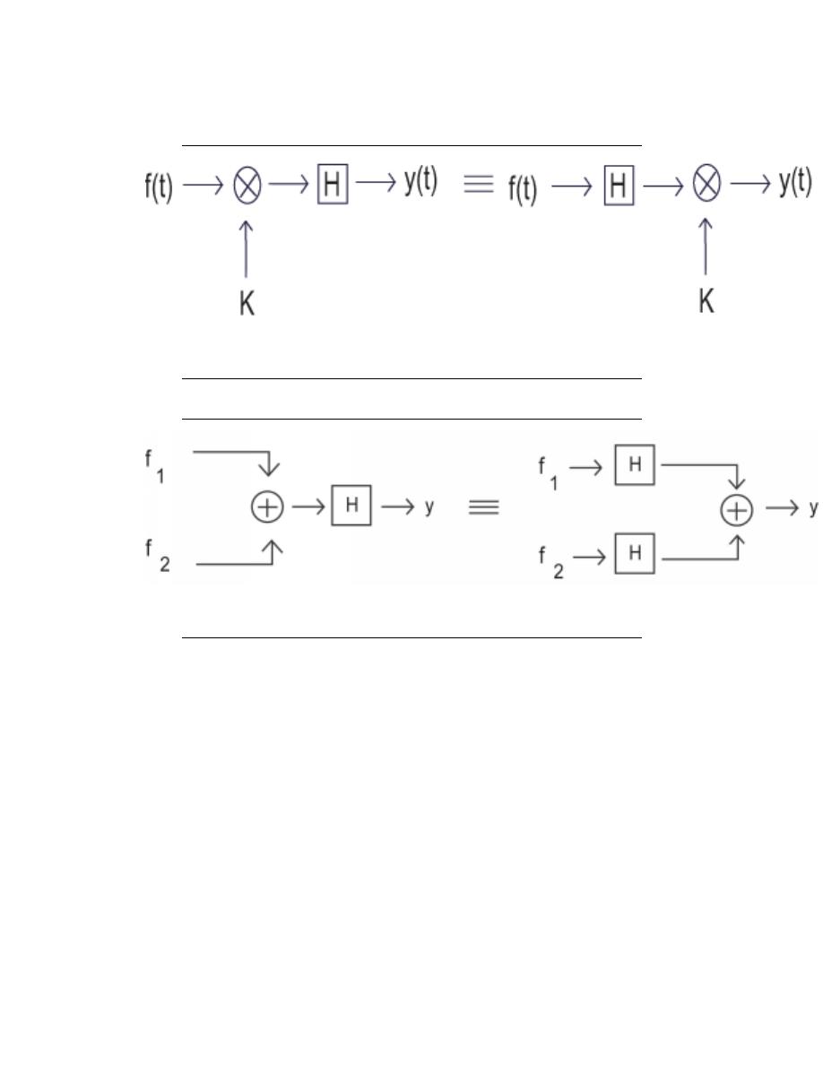
2.1.2.2 Linear vs. Nonlinear
A linear system is any system that obeys the properties of scaling (homogeneity) and
superposition (additivity), while a nonlinear system is any system that does not obey at
least one of these.
To show that a system H obeys the scaling property is to show that
H (kf (t)) = kH (f (t))
(2.1)
7
8
CHAPTER 2. SIGNALS AND SYSTEMS: A FIRST LOOK
Figure 2.1: A block diagram demonstrating the scaling property of linearity
Figure 2.2: A block diagram demonstrating the superposition property of linearity
To demonstrate that a system H obeys the superposition property of linearity is to show
that
H (f
1
(t) + f
2
(t)) = H (f
1
(t)) + H (f
2
(t))
(2.2)
It is possible to check a system for linearity in a single (though larger) step. To do this,
simply combine the first two steps to get
H (k
1
f
1
(t) + k
2
f
2
(t)) = k
2
H (f
1
(t)) + k
2
H (f
2
(t))
(2.3)
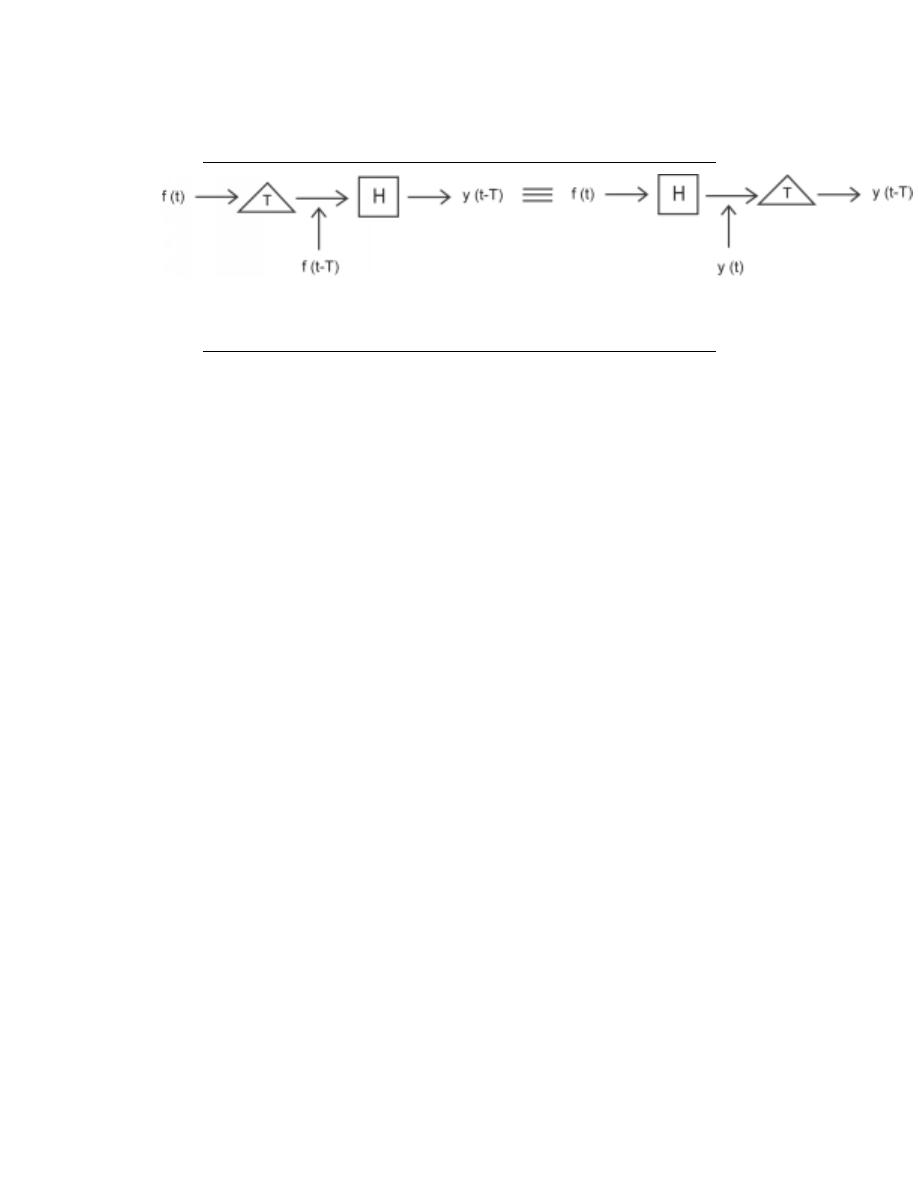
2.1.2.3 Time Invariant vs. Time Variant
A time invariant system is one that does not depend on when it occurs: the shape of the
output does not change with a delay of the input. That is to say that for a system H where
H (f (t)) = y (t), H is time invariant if for all T
H (f (t − T )) = y (t − T )
(2.4)
9
Figure 2.3:
This block diagram shows what the condition for time invariance. The
output is the same whether the delay is put on the input or the output.
When this property does not hold for a system, then it is said to be time variant , or
time-varying.
2.1.2.4 Causal vs. Noncausal
A causal system is one that is nonanticipative ; that is, the output may depend on current
and past inputs, but not future inputs. All ”realtime” systems must be causal, since they
can not have future inputs available to them.
One may think the idea of future inputs does not seem to make much physical sense;
however, we have only been dealing with time as our dependent variable so far, which is
not always the case. Imagine rather that we wanted to do image processing. Then the
dependent variable might represent pixels to the left and right (the ”future”) of the current
position on the image, and we would have a noncausal system.
2.1.2.5 Stable vs. Unstable
A stable system is one where the output does not diverge as long as the input does not
diverge. A bounded input produces a bounded output. It is from this property that this
type of system is referred to as bounded input-bounded output (BIBO) stable.
Representing this in a mathematical way, a stable system must have the following prop-
erty, where x (t) is the input and y (t) is the output. The output must satisfy the condition
|y (t) | ≤ M
y
< ∞
(2.5)
when we have an input to the system that can be described as
|x (t) | ≤ M
x
< ∞
(2.6)
M
x
and M
y
both represent a set of finite positive numbers and these relationships hold for
all of t.
If these conditions are not met, i.e. a system’s output grows without limit (diverges)
from a bounded input, then the system is unstable .
3.2 Properties of Systems
2.2.1 ”Linear Systems”
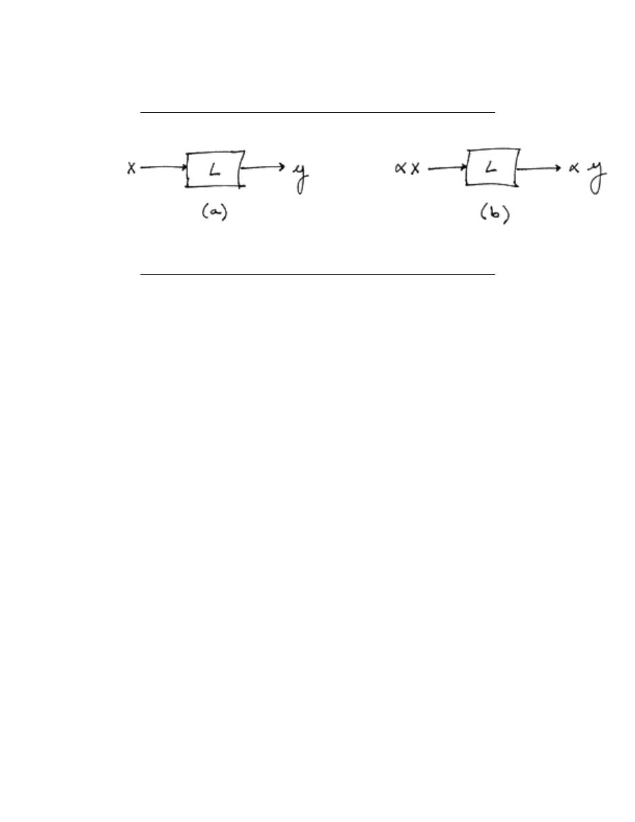
If a system is linear, this means that when an input to a given system is scaled by a value,
the output of the system is scaled by the same amount.
10
CHAPTER 2. SIGNALS AND SYSTEMS: A FIRST LOOK
(a)
(b)
Figure 2.4:
(a) For a typical system to be causal... (b) ...the output at time t
0
, y (t
0
),
can only depend on the portion of the input signal before t
0
.
11
Linear Scaling
Figure 2.5
In part (a) of the figure above, an input x to the linear system L gives the output y If x
is scaled by a value α and passed through this same system, as in part (b), the output will
also be scaled by α.
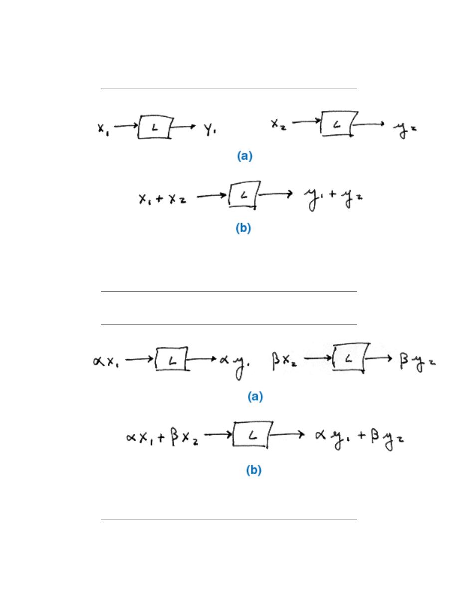
A linear system also obeys the principle of superposition. This means that if two inputs
are added together and passed through a linear system, the output will be the sum of the
individual inputs’ outputs.
That is, if (a) is true, then (b) is also true for a linear system. The scaling property
mentioned above still holds in conjunction with the superposition principle. Therefore, if
the inputs x and y are scaled by factors α and β, respectively, then the sum of these scaled
inputs will give the sum of the individual scaled outputs:
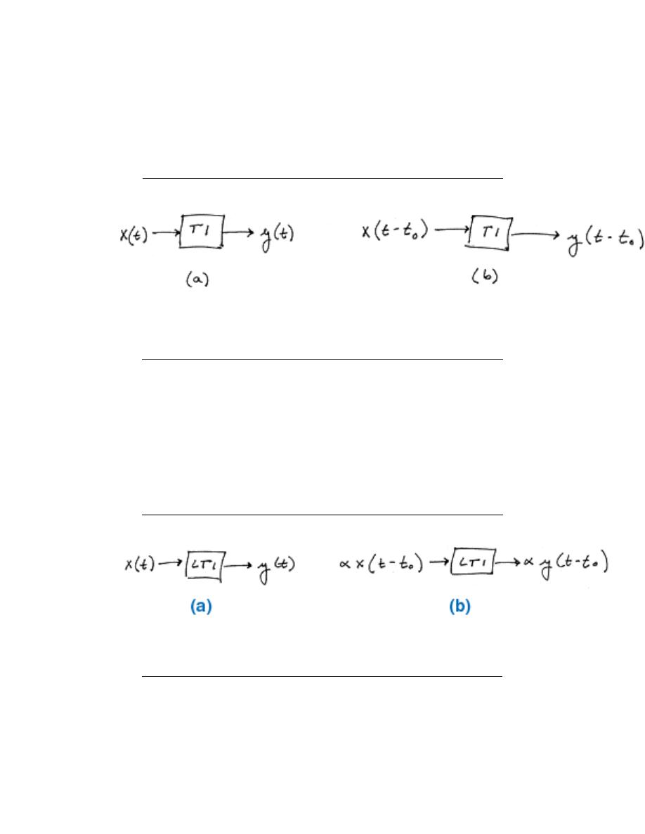
2.2.2 ”Time-Invariant Systems”
A time-invariant system has the property that a certain input will always give the same
output, without regard to when the input was applied to the system.
In this figure, x (t) and x (t − t
0
) are passed through the system TI. Because the system
TI is time-invariant, the inputs x (t) and x (t − t
0
) produce the same output. The only
difference is that the output due to x (t − t
0
) is shifted by a time t
0
.
Whether a system is time-invariant or time-varying can be seen in the differential equa-
tion (or difference equation) describing it. Time-invariant systems are modeled with constant
coefficient equations. A constant coefficient differential (or difference) equation means that
the parameters of the system are not changing over time and an input now will give the
same result as the same input later.
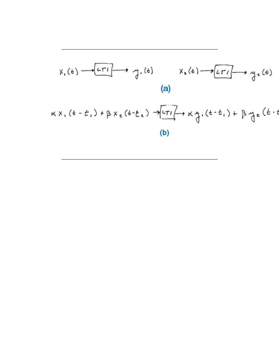
2.2.3 ”Linear Time-Invariant (LTI) Systems”
Certain systems are both linear and time-invariant, and are thus referred to as LTI systems.
As LTI systems are a subset of linear systems, they obey the principle of superposition. In
the figure below, we see the effect of applying time-invariance to the superposition definition
in the linear systems section above.
12
CHAPTER 2. SIGNALS AND SYSTEMS: A FIRST LOOK
Superposition Principle
Figure 2.6: If (a) is true, then the principle of superposition says that (b) is true as
well. This holds for linear systems.
Superposition Principle with Linear Scaling
Figure 2.7: Given (a) for a linear system, (b) holds as well.
13
Time-Invariant Systems
Figure 2.8: (a) shows an input at time t while (b) shows the same input t
0
seconds
later. In a time-invariant system both outputs would be identical except that the one in
(b) would be delayed by t
0
.
Linear Time-Invariant Systems
Figure 2.9: This is a combination of the two cases above. Since the input to (b) is a
scaled, time-shifted version of the input in (a), so is the output.
14
CHAPTER 2. SIGNALS AND SYSTEMS: A FIRST LOOK
Superposition in Linear Time-Invariant Systems
Figure 2.10: The principle of superposition applied to LTI systems
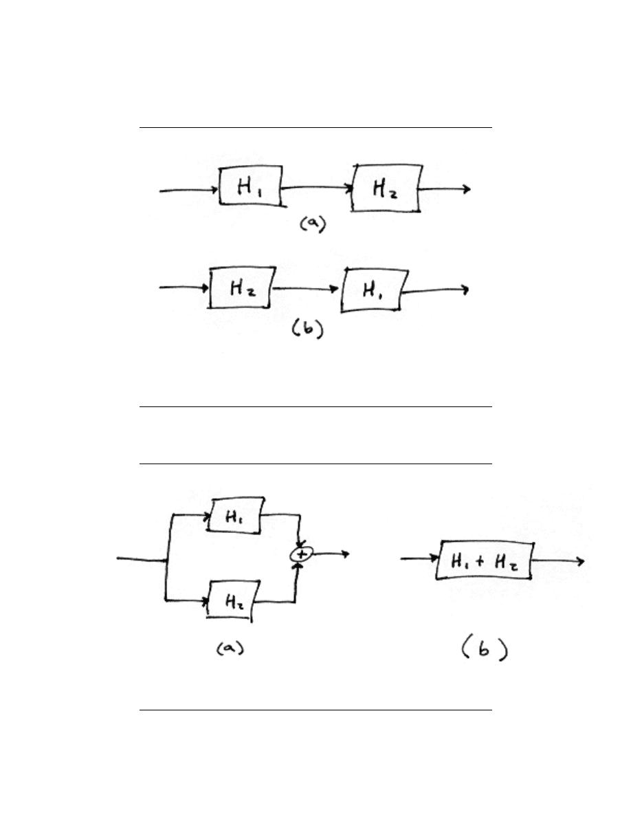
2.2.3.1 ”LTI Systems in Series”
If two or more LTI systems are in series with each other, their order can be interchanged
without affecting the overall output of the system. Systems in series are also called cascaded
systems.
2.2.3.2 ”LTI Systems in Parallel”
If two or more LTI systems are in parallel with one another, an equivalent system is one
that is defined as the sum of these individual systems.
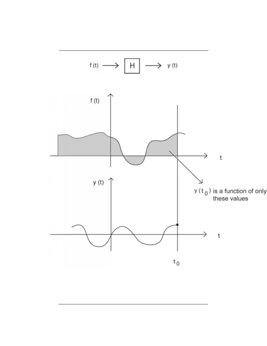
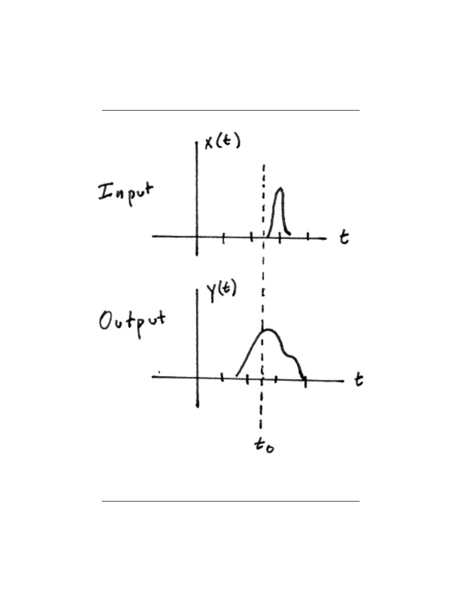
2.2.4 ”Causality”
A system is causal if it does not depend on future values of the input to determine the
output. This means that if the first input to a system comes at time t
0
, then the system
should not give any output until that time. An example of a non-causal system would be
one that ”sensed” an input coming and gave an output before the input arrived:
A causal system is also characterized by an impulse response h(t) that is zero for t <0.
3.3 Signal Classifications and Properties
2.3.1 Introduction
This module will lay out some of the fundamentals of signal classification. This is basically
a list of definitions and properties that are fundamental to the discussion of signals and
systems. It should be noted that some discussions like energy signals vs. power signals have
been designated their own module for a more complete discussion, and will not be included
here.
15
Cascaded LTI Systems
Figure 2.11: The order of cascaded LTI systems can be interchanged without changing
the overall effect.
Parallel LTI Systems
Figure 2.12: Parallel systems can be condensed into the sum of systems.
16
CHAPTER 2. SIGNALS AND SYSTEMS: A FIRST LOOK
Non-causal System
Figure 2.13: In this non-causal system, an output is produced due to an input that
occurs later in time.
17
Figure 2.14
2.3.2 Classifications of Signals
Along with the classification of signals below, it is also important to understand the Clas-
sification of Systems.
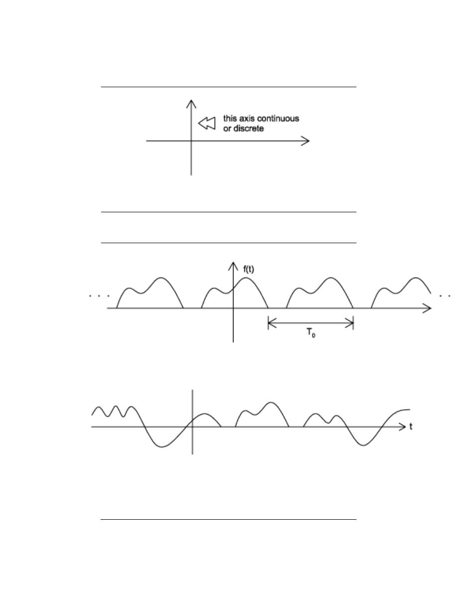
2.3.2.1 Continuous-Time vs. Discrete-Time
As the names suggest, this classification is determined by whether or not the time axis
(x-axis) is discrete (countable) or continuous . A continuous-time signal will contain a
value for all real numbers along the time axis. In contrast to this, a discrete-time signal is
often created by using the sampling theorem to sample a continuous signal, so it will only
have values at equally spaced intervals along the time axis.
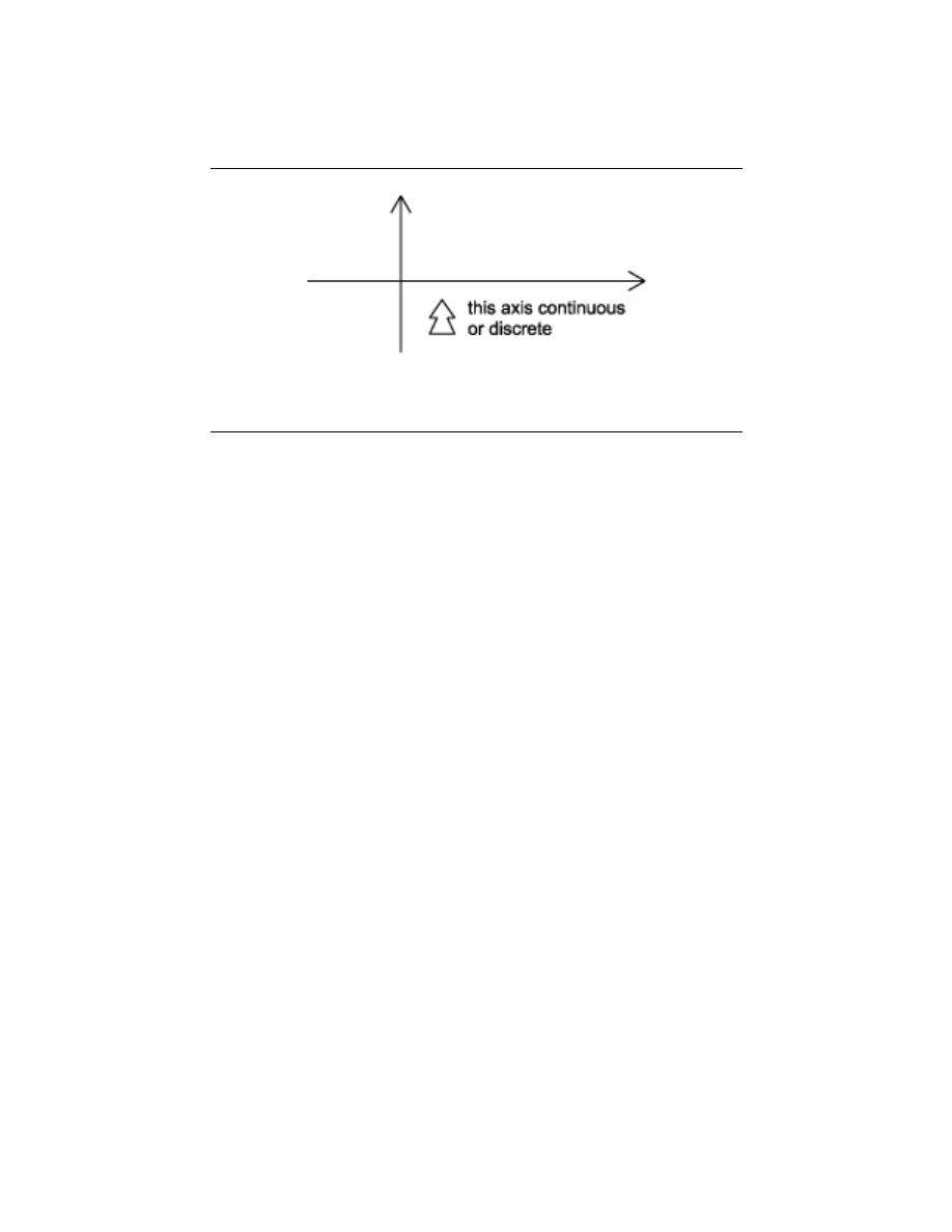
2.3.2.2 Analog vs. Digital
The difference between analog and digital is similar to the difference between continuous-
time and discrete-time. In this case, however, the difference is with respect to the value of
the function (y-axis). Analog corresponds to a continuous y-axis, while digital corresponds
to a discrete y-axis. An easy example of a digital signal is a binary sequence, where the
values of the function can only be one or zero.
2.3.2.3 Periodic vs. Aperiodic
Periodic signals repeat with some period T, while aperiodic, or nonperiodic, signals do not.
We can define a periodic function through the following mathematical expression, where t
can be any number and T is a positive constant:
f (t) = f (T + t)
(2.7)
The fundamental period of our function, f (t), is the smallest value of T that the still
allows the above equation, Equation 2.7, to be true.
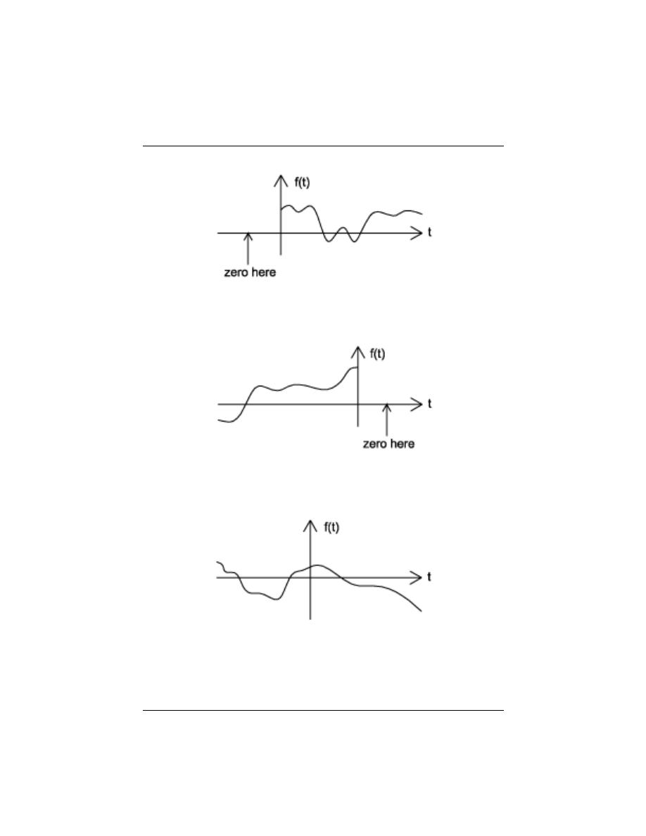
2.3.2.4 Causal vs. Anticausal vs. Noncausal
Causal signals are signals that are zero for all negative time, while anitcausal are signals
that are zero for all positive time. Noncausal signals are signals that have nonzero values
in both positive and negative time.
18
CHAPTER 2. SIGNALS AND SYSTEMS: A FIRST LOOK
Figure 2.15
(a)
(b)
Figure 2.16:
(a) A periodic signal with period T
0
(b) An aperiodic signal
19
(a)
(b)
(c)
Figure 2.17:
(a) A causal signal (b) An anticausal signal (c) A noncausal signal
20
CHAPTER 2. SIGNALS AND SYSTEMS: A FIRST LOOK
(a)
(b)
Figure 2.18:
(a) An even signal (b) An odd signal
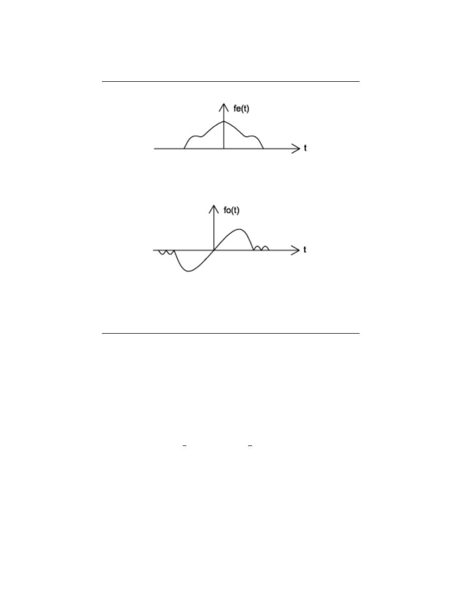
2.3.2.5 Even vs. Odd
An even signal is any signal f such that f (t) = f (−t). Even signals can be easily spotted
as they are symmetric around the vertical axis. An odd signal , on the other hand, is a
signal f such that f (t) = − (f (−t)).
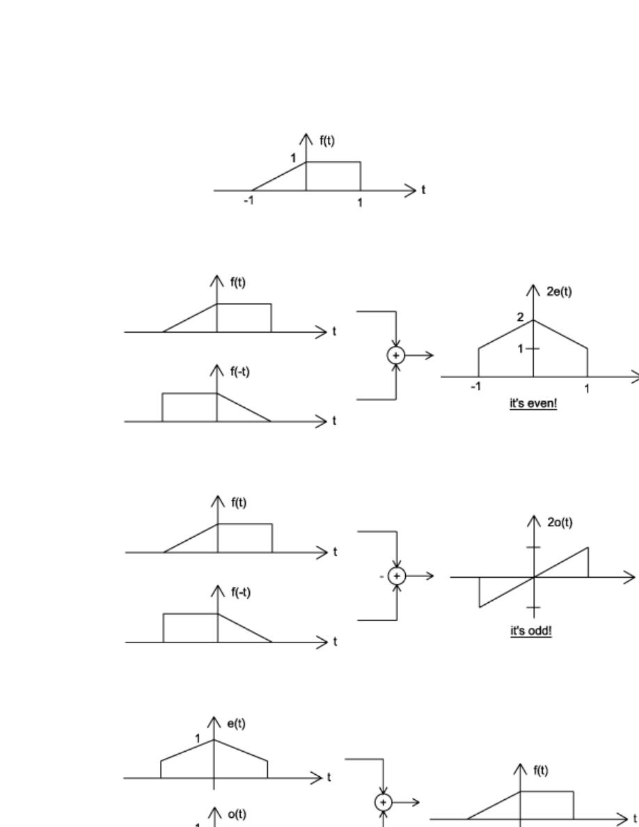
Using the definitions of even and odd signals, we can show that any signal can be
written as a combination of an even and odd signal. That is, every signal has an odd-even
decomposition. To demonstrate this, we have to look no further than a single equation.
f (t) =
1
2
(f (t) + f (−t)) +
1
2
(f (t) − f (−t))
(2.8)
By multiplying and adding this expression out, it can be shown to be true. Also, it can be
shown that f (t) + f (−t) fulfills the requirement of an even function, while f (t) − f (−t)
fulfills the requirement of an odd function.
Example 2.1:
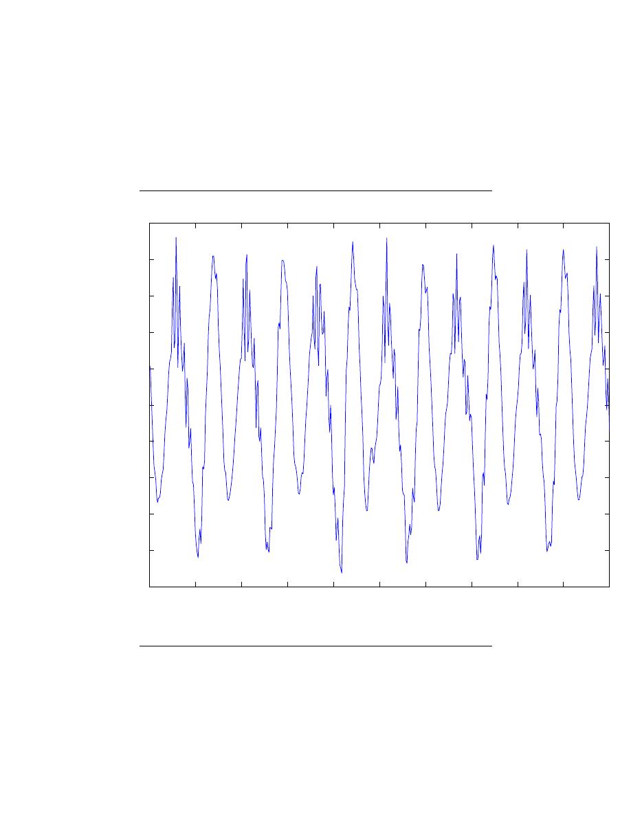
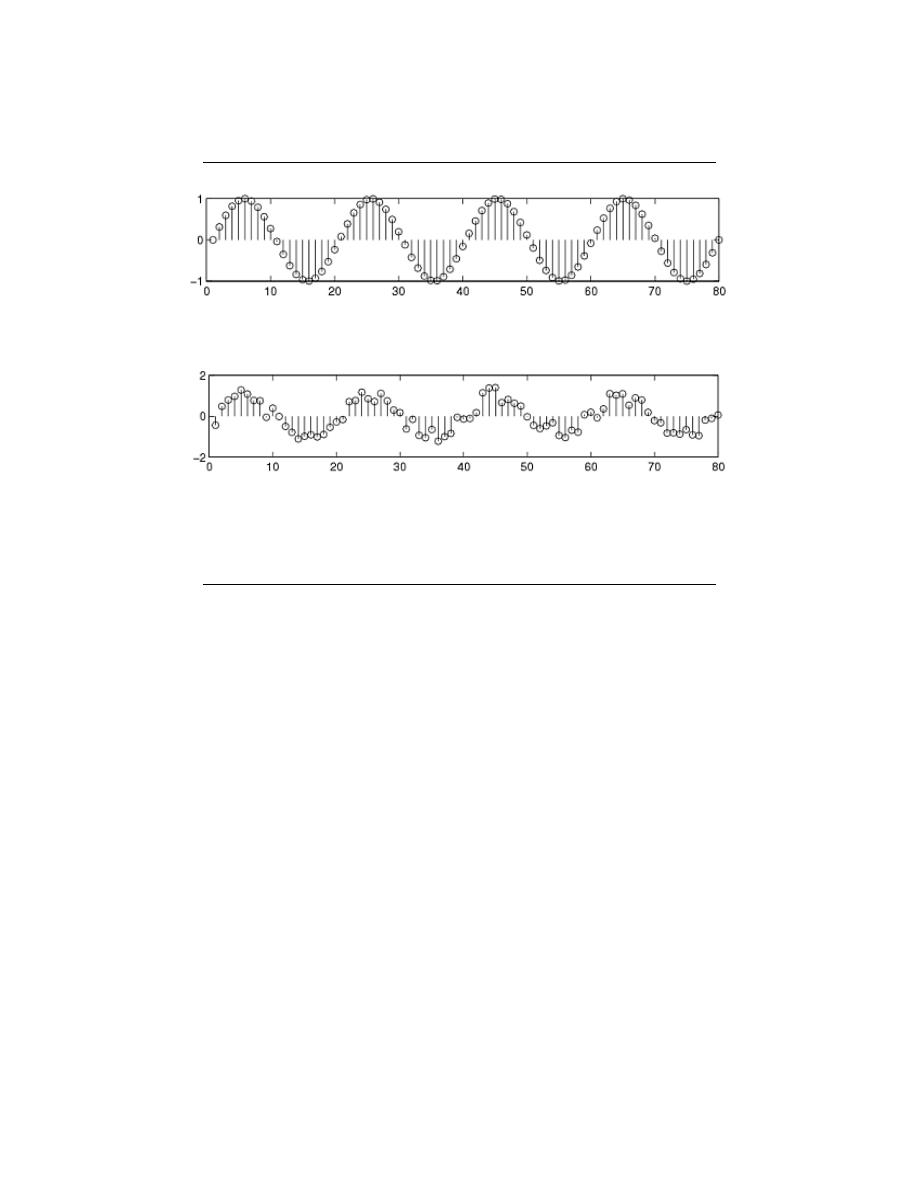
2.3.2.6 Deterministic vs. Random
A deterministic signal is a signal in which each value of the signal is fixed and can be
determined by a mathematical expression, rule, or table. Because of this the future values
21
(a)
(b)
(c)
(d)
Figure 2.19:
(a) The signal we will decompose using odd-even decomposition (b)
Even part: e (t) =
1
2
(f (t) + f (−t)) (c) Odd part: o (t) =
1
2
(f (t) − f (−t)) (d) Check:
e (t) + o (t) = f (t)
22
CHAPTER 2. SIGNALS AND SYSTEMS: A FIRST LOOK
(a)
(b)
Figure 2.20:
(a) Deterministic Signal (b) Random Signal
of the signal can be calculated from past values with complete confidence. On the other
hand, a random signal has a lot of uncertainty about its behavior. The future values of a
random signal cannot be acurately predicted and can usually only be guessed based on the
averages of sets of signals.
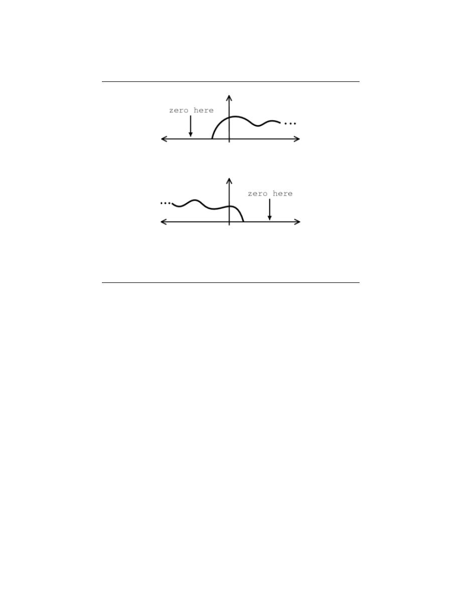
2.3.2.7 Right-Handed vs. Left-Handed
A right-handed signal and left-handed signal are those signals whose value is zero between
a given variable and positive or negative infinity. Mathematically speaking, a right-handed
signal is defined as any signal where f (t) = 0 for t < t
1
< ∞, and a left-handed signal
is defined as any signal where f (t) = 0 for t > t
1
> −∞. See the figures below for an
example. Both figures ”begin” at t
1
and then extends to positive or negative infinity with
mainly nonzero values.
2.3.2.8 Finite vs. Infinite Length
As the name applies, signals can be characterized as to whether they have a finite or infinite
length set of values. Most finite length signals are used when dealing with discrete-time
signals or a given sequence of values. Mathematically speaking, f (t) is a finite-length
signal if it is nonzero over a finite interval
t
1
< f (t) < t
2
where t
1
> −∞ and t
2
< ∞. An example can be seen in the below figure. Similarly, an
infinite-length signal , f (t), is defined as nonzero over all real numbers:
∞ ≤ f (t) ≤ −∞
23
(a)
(b)
Figure 2.21:
(a) Right-handed signal (b) Left-handed signal
3.4 Discrete-Time Signals
So far, we have treated what are known as analog signals and systems. Mathematically,
analog signals are functions having countinuous quantities as their independent variables,
such as space and time. Discrete-time signals are functions defined on the integers; they
are sequences. One of the fundamental results of signal theory will detail conditions under
which an analog signal can be converted into a discrete-time one and retrieved without
error. This result is important because discrete-time signals can be manipulated by systems
instantiated as computer programs. Subsequent modules describe how virtually all analog
signal processing can be performed with software.
As important as such results are, discrete-time signals are more general, encompassing
signals derived from analog ones and
signals that aren’t. For example, the characters
forming a text file form a sequence, which is also a discrete-time signal. We must deal with
such symbolic valued (pg ??) signals and systems as well.
As with analog signals, we seek ways of decomposing real-valued discrete-time signals
into simpler components. With this approach leading to a better understanding of signal
structure, we can exploit that structure to represent information (create ways of repre-
senting information with signals) and to extract information (retrieve the information thus
represented). For symbolic-valued signals, the approach is different: We develop a common
representation of all symbolic-valued signals so that we can embody the information they
contain in a unified way. From an information representation perspective, the most impor-
tant issue becomes, for both real-valued and symbolic-valued signals, efficiency; What is the
most parsimonious and compact way to represent information so that it can be extracted
24
CHAPTER 2. SIGNALS AND SYSTEMS: A FIRST LOOK
Figure 2.22: Finite-Length Signal. Note that it only has nonzero values on a set, finite
interval.
later.
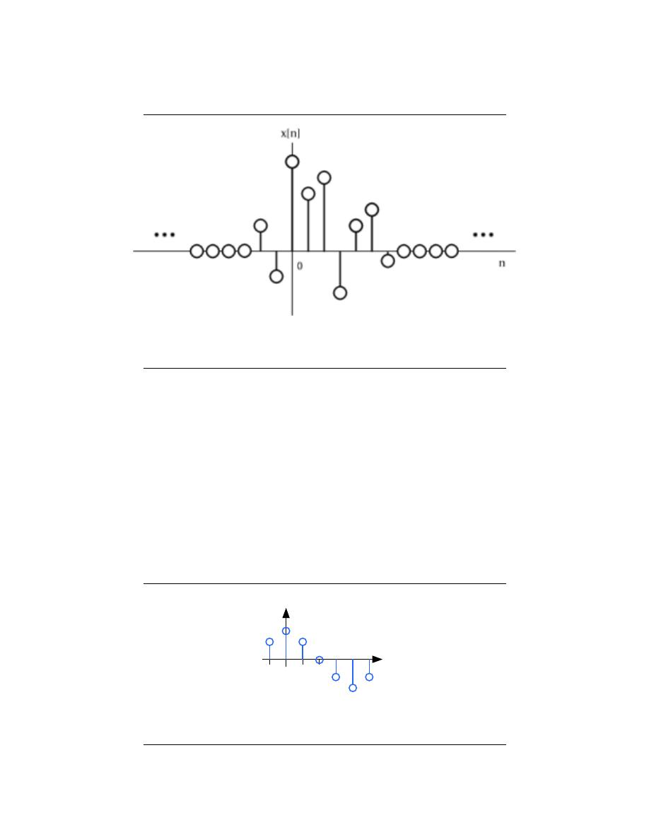
2.4.1 Real- and Complex-valued Signals
A discrete-time signal is represented symbolically as s (n), where n = {. . . , −1, 0, 1, . . . }.
We usually draw discrete-time signals as stem plots to emphasize the fact they are functions
defined only on the integers. We can delay a discrete-time signal by an integer just as with
analog ones. A delayed unit sample has the expression δ (n − m), and equals one when
n = m.
Discrete-Time Cosine Signal
n
sn
1
…
…
Figure 2.23:
The discrete-time cosine signal is plotted as a stem plot. Can you find
the formula for this signal?

25
Unit Sample
1
n
δ
n
Figure 2.24: The unit sample.
2.4.2 Complex Exponentials
The most important signal is, of course, the complex exponential sequence .
s (n) = e
j2πf n
(2.9)
2.4.3 Sinusoids
Discrete-time sinusoids have the obvious form s (n) = Acos (2πf n + φ). As opposed to
analog complex exponentials and sinusoids that can have their frequencies be any real value,
frequencies of their discrete-time counterparts yield unique waveforms only when f lies in
the interval −
1
2
,
1
2
. This property can be easily understood by noting that adding an
integer to the frequency of the discrete-time complex exponential has no effect on the signal’s
value.
e
j2π(f +m)n
=
e
j2πf n
e
j2πmn
=
e
j2πf n
(2.10)
This derivation follows because the complex exponential evaluated at an integer multiple of
2π equals one.
2.4.4 Unit Sample
The second-most important discrete-time signal is the unit sample , which is defined to
be
δ (n) =
1 if n = 0
0 otherwise
(2.11)
Examination of a discrete-time signal’s plot, like that of the cosine signal shown in this
figure (Figure 2.23), reveals that all signals consist of a sequence of delayed and scaled unit
samples. Because the value of a sequence at each integer m is denoted by s (m) and the
unit sample delayed to occur at m is written δ (n − m), we can decompose any signal as a
sum of unit samples delayed to the appropriate location and scaled by the signal value.
s (n) =
∞
X
m=−∞
(s (m) δ (n − m))
(2.12)
This kind of decomposition is unique to discrete-time signals, and will prove useful subse-
quently.
Discrete-time systems can act on discrete-time signals in ways similar to those found in
analog signals and systems. Because of the role of software in discrete-time systems, many

26
CHAPTER 2. SIGNALS AND SYSTEMS: A FIRST LOOK
more different systems can be envisioned and “constructed” with programs than can be
with analog signals. In fact, a special class of analog signals can be converted into discrete-
time signals, processed with software, and converted back into an analog signal, all without
the incursion of error. For such signals, systems can be easily produced in software, with
equivalent analog realizations difficult, if not impossible, to design.
2.4.5 Symbolic-valued Signals
Another interesting aspect of discrete-time signals is that their values do not need to be
real numbers. We do have real-valued discrete-time signals like the sinusoid, but we also
have signals that denote the sequence of characters typed on the keyboard. Such characters
certainly aren’t real numbers, and as a collection of possible signal values, they have little
mathematical structure other than that they are members of a set. More formally, each
element of the symbolic-valued signal s (n) takes on one of the values {a
1
, . . . , a
K
} which
comprise the alphabet A. This technical terminology does not mean we restrict symbols
to being members of the English or Greek alphabet. They could represent keyboard char-
acters, bytes (8-bit quantities), integers that convey daily temperature. Whether controlled
by software or not, discrete-time systems are ultimately constructed from digital circuits,
which consist entirely of analog circuit elements. Furthermore, the transmission and recep-
tion of discrete-time signals, like e-mail, is accomplished with analog signals and systems.
Understanding how discrete-time and analog signals and systems intertwine is perhaps the
main goal of this course.
3.5 Useful Signals
Before looking at this module, hopefully you have some basic idea of what a signal is and
what basic classifications and properties a signal can have. To review, a signal is merely a
function defined with respect to an independent variable. This variable is often time but
could represent an index of a sequence or any number of things in any number of dimensions.
Most, if not all, signals that you will encounter in your studies and the real world will be
able to be created from the basic signals we discuss below. Because of this, these elementary
signals are often referred to as the building blocks for all other signals.
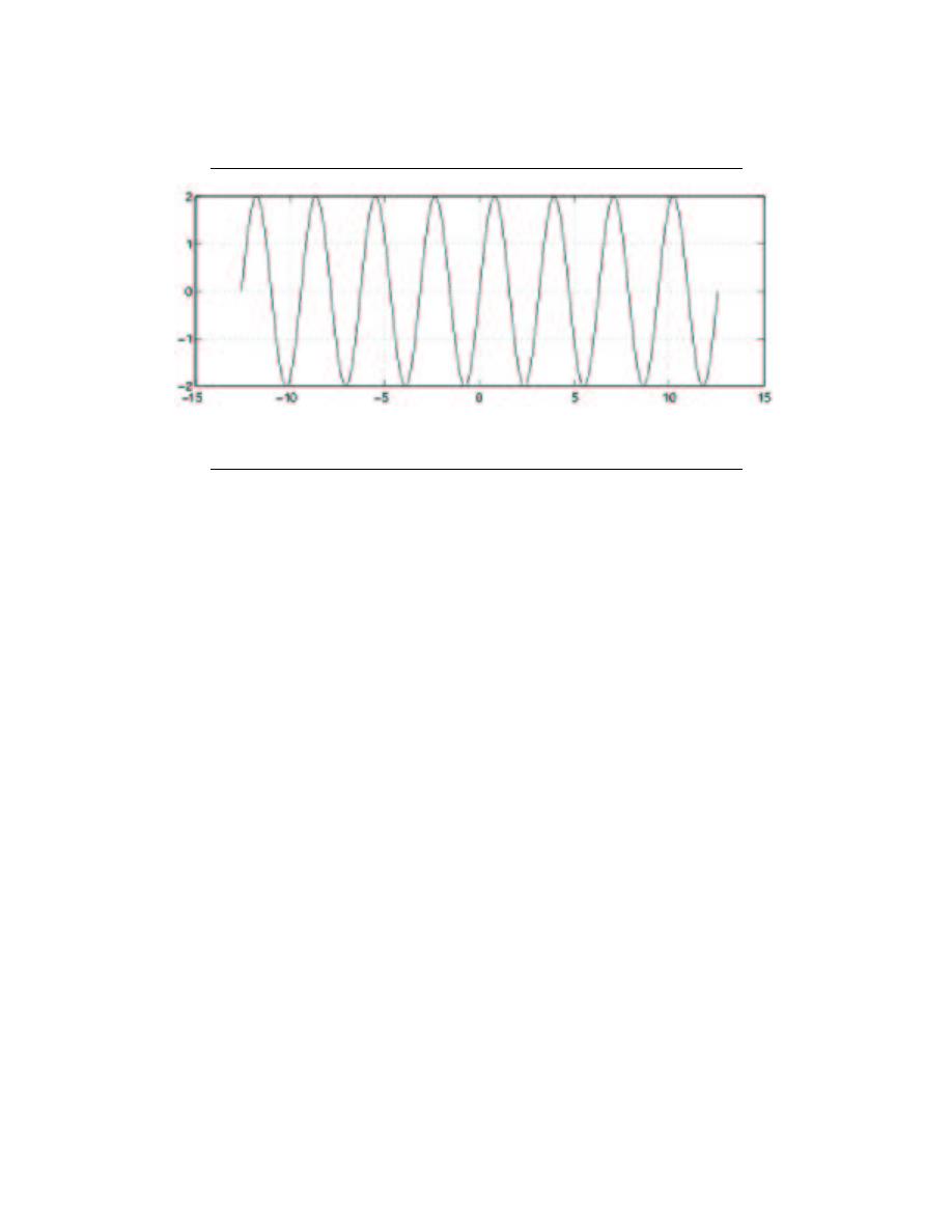
2.5.1 Sinusoids
Probably the most important elemental signal that you will deal with is the real-valued
sinusoid. In its continuous-time form, we write the general form as
x (t) = Acos (ωt + φ)
(2.13)
where A is the amplitude, ω is the frequency, and φ represents the phase. Note that it is
common to see ωt replaced with 2πf t. Since sinusoidal signals are periodic, we can express
the period of these, or any periodic signal, as
T =
2π
ω
(2.14)
2.5.2 Complex Exponential Function
Maybe as important as the general sinusoid, the complex exponential function will be-
come a critical part of your study of signals and systems. Its general form is written as
27
Figure 2.25:
Sinusoid with A = 2, w = 2, and φ = 0.
f (t) = Be
st
(2.15)
where s, shown below, is a complex number in terms of σ, the phase constant, and ω the
frequency:
s = σ + jω
Please look at the complex exponential module or the other elemental signals page (pg ??)
for a much more in depth look at this important signal.
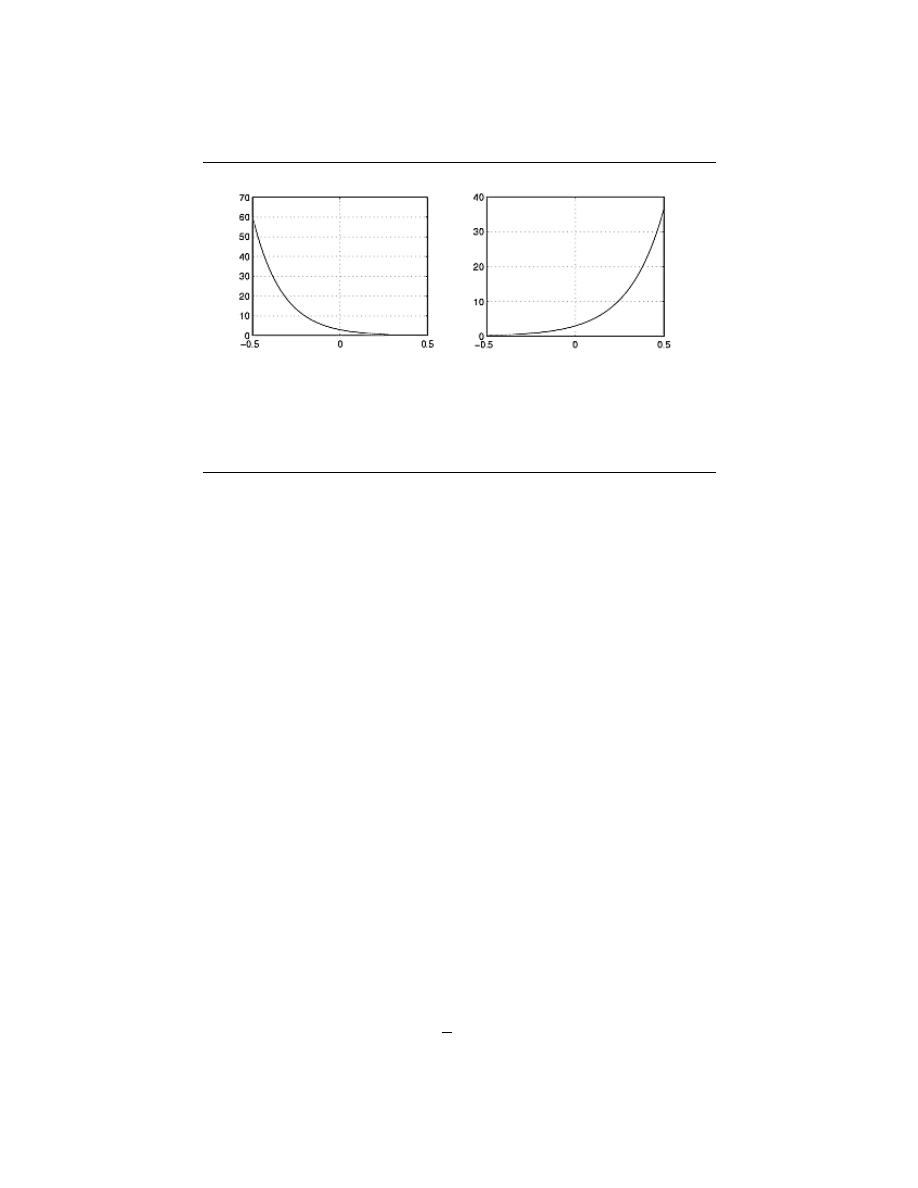
2.5.3 Real Exponentials
Just as the name sounds, real exponentials contain no imaginary numbers and are expressed
simply as
f (t) = Be
αt
(2.16)
where both B and α are real parameters. Unlike the complex exponential that oscillates,
the real exponential either decays or grows depending on the value of α.
• - Decaying Exponential , when α < 0
• - Growing Exponential , when α > 0
2.5.4 Unit Impulse Function
The unit impulse ”function” (or Dirac delta function) is a signal that has infinite height
and infinitesimal width. However, because of the way it is defined, it actually integrates to
one. While in the engineering world, this signal is quite nice and aids in the understanding of
many concepts, some mathematicians have a problem with it being called a function, since
it is not defined at t = 0 . Engineers reconcile this problem by keeping it around integrals,
in order to keep it more nicely defined. The unit impulse is most commonly denoted as
δ (t)
28
CHAPTER 2. SIGNALS AND SYSTEMS: A FIRST LOOK
(a)
(b)
Figure 2.26:
Examples of Real Exponentials (a) Decaying Exponential (b) Growing
Exponential
The most important property of the unit-impulse is shown in the following integral:
Z
∞
−∞
δ (t) dt = 1
(2.17)
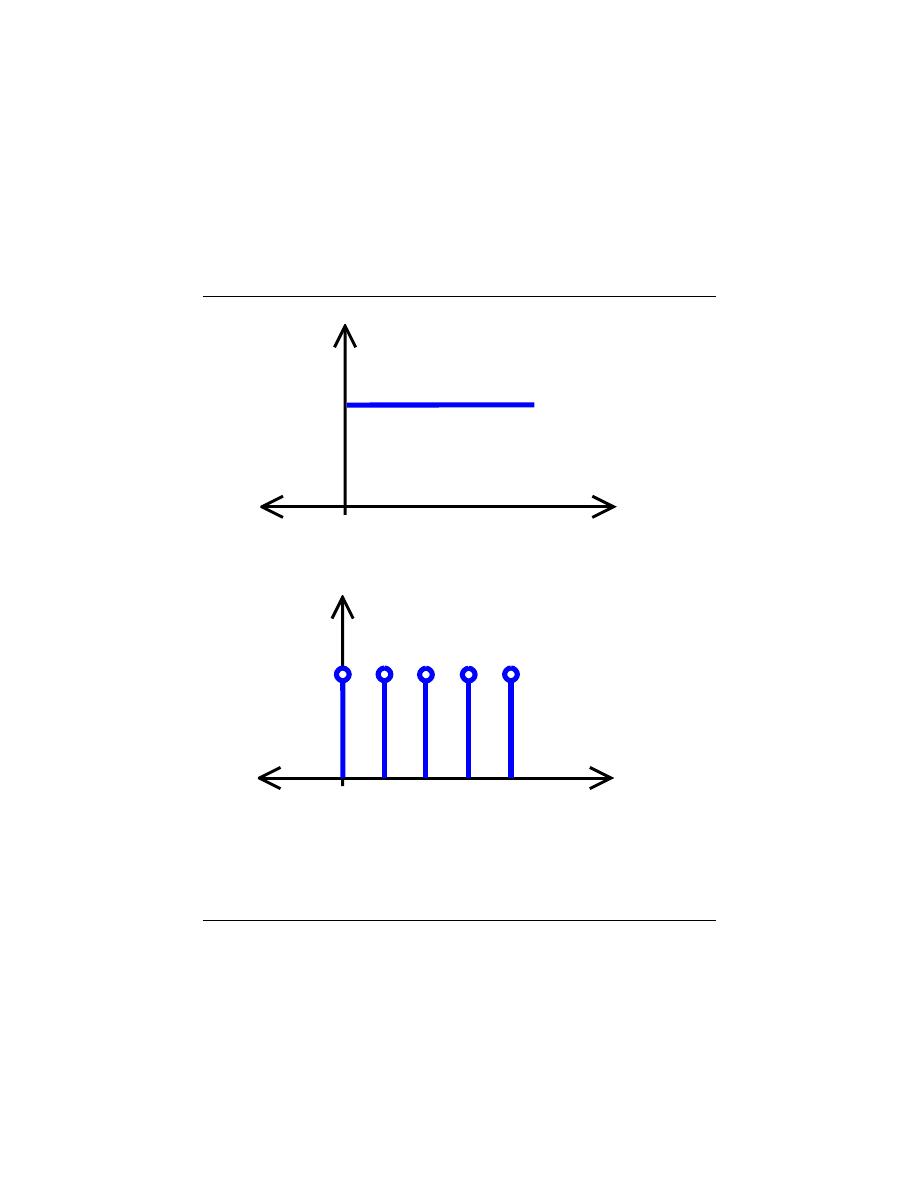
2.5.5 Unit-Step Function
Another very basic signal is the unit-step function that is defined as
u (t) =
1 if t < 0
0 if t ≥ 0
(2.18)
Note that the step function is discontinuous at the origin; however, it does not need to
be defined here as it does not matter in signal theory. The step function is a useful tool for
testing and for defining other signals. For example, when different shifted versions of the
step function are multiplied by other signals, one can select a certain portion of the signal
and zero out the rest.
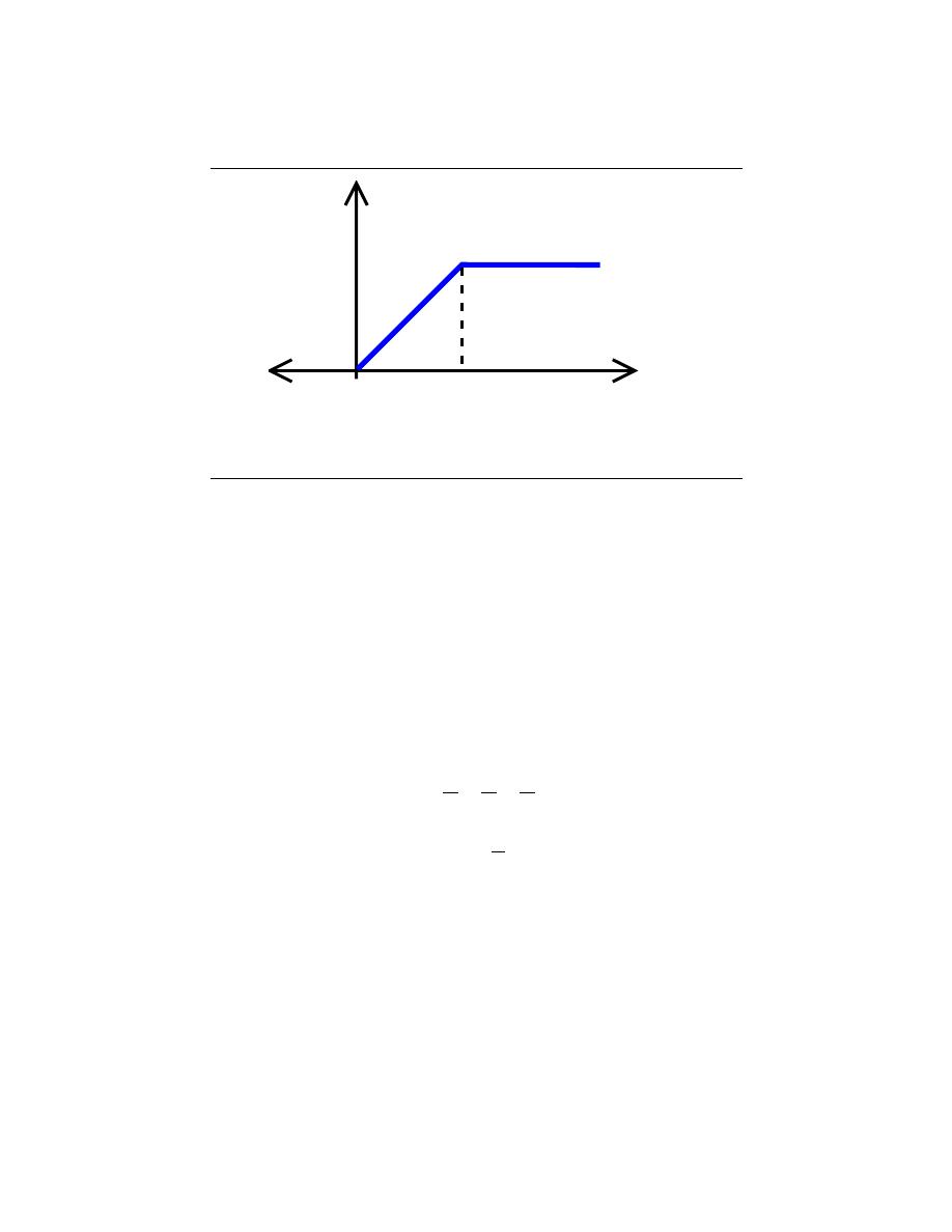
2.5.6 Ramp Function
The ramp function is closely related to the unit-step discussed above. Where the unit-
step goes from zero to one instantaneously, the ramp function better resembles a real-world
signal, where there is some time needed for the signal to increase from zero to its set value,
one in this case. We define a ramp function as follows
r (t) =
0 if t < 0
t
t
0
if 0 ≤ t ≤ t
0
1 if t > t
0
(2.19)
29
t
1
(a)
t
1
(b)
Figure 2.27:
Basic Step Functions (a) Continuous-Time Unit-Step Function (b)
Discrete-Time Unit-Step Function
30
CHAPTER 2. SIGNALS AND SYSTEMS: A FIRST LOOK
t
1
t
0
Figure 2.28:
Ramp Function
3.6 The Complex Exponential
2.6.1 The Exponential Basics
The complex exponential is one of the most fundamental and important signal in signal
and system analysis. Its importance comes from its functions as a basis for periodic signals
as well as being able to characterize linear, time-invariant signals. Before proceeding, you
should be familiar with the ideas and functions of complex numbers.
2.6.1.1 Basic Exponential
For all numbers x, we easily derive and define the exponential function from the Taylor’s
series below:
e
x
= 1 +
x
1
1!
+
x
2
2!
+
x
3
3!
+ . . .
(2.20)
e
x
=
∞
X
k=0
1
k!
x
k
(2.21)
We can prove, using the ratio test, that this series does indeed converge. Therefore, we can
state that the exponential function shown above is continuous and easily defined.
From this definition, we can prove the following property for exponentials that will be
very useful, especially for the complex exponentials discussed in the next section.
e
x
1
+x
2
= (e
x
1
) (e
x
2
)
(2.22)
2.6.1.2 Complex Continuous-Time Exponential
Now for all complex numbers s, we can define the complex continuous-time exponential
signal as
f (t)
=
Ae
st
=
Ae
jωt
(2.23)

31
where A is a constant, t is our independent variable for time, and for s imaginary, s = jω.
Finally, from this equation we can reveal the ever important Euler’s Identity (for more
information on Euler read this short biography
1
):
Ae
jωt
= Acos (ωt) + j (Asin (ωt))
(2.24)
From Euler’s Identity we can easily break the signal down into its real and imaginary
components. Also we can see how exponentials can be combined to represet any real signal.
By modifying their frequency and phase, we can represent any signal through a superposity
of many signals - all capable of being represented by an exponential.
The above expressions do not include any information on phase however. We can further
generalize our above expressions for the exponential to generalize sinusoids with any phase
by making a final substitution for s, s = σ + jω, which leads us to
f (t)
=
Ae
st
=
Ae
(σ+jω)t
=
Ae
σt
e
jωt
(2.25)
where we define S as the complex amplitude , or phasor , from the first two terms of
the above equation as
S = Ae
σt
(2.26)
Going back to Euler’s Identity, we can rewrite the exponentials as sinusoids, where the phase
term becomes much more apparent.
f (t)
=
Ae
σt
(cos (ωt) + jsin (ωt))
=
Acos (σ + ωt) + jAsin (σ + ωt)
(2.27)
As stated above we can easily break this formula into its real and imaginary part as follows:
Re (f (t)) = Ae
σt
cos (ωt)
(2.28)
Im (f (t)) = Ae
σt
sin (ωt)
(2.29)
2.6.1.3 Complex Discrete-Time Exponential
Finally we have reached the last form of the exponential signal that we will be interested
in, the discrete-time exponential signal , which we will not give as much detail about
as we did for its continuous-time counterpart, because they both follow the same properties
and logic discussed above. Because it is discrete, there is only a slightly different notation
used to represents its discrete nature
f [n]
=
Be
snT
=
Be
jωnT
(2.30)
where nT represents the discrete-time instants of our signal.
2.6.2 Euler’s Relation
Along with Euler’s Identity, Euler also described a way to represent a complex exponential
signal in terms of its real and imaginary parts through Euler’s Relation :
cos (ωt) =
e
jwt
+ e
−(jwt)
2
(2.31)
1
http://www-groups.dcs.st-and.ac.uk/∼history/Mathematicians/Euler.html
32
CHAPTER 2. SIGNALS AND SYSTEMS: A FIRST LOOK
(a)
(b)
(c)
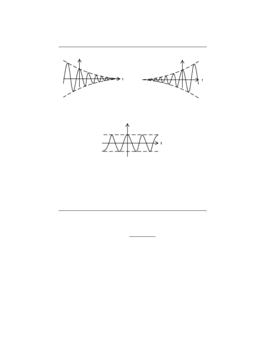
Figure 2.29:
The shapes possible for the real part of a complex exponential. Notice
that the oscillations are the result of a cosine, as there is a local maximum at t = 0. (a)
If σ is negative, we have the case of a decaying exponential window. (b) If σ is positive,
we have the case of a growing exponential window. (c) If σ is zero, we have the case of a
constant window.
sin (ωt) =
e
jwt
− e
−(jwt)
2j
(2.32)
e
jwt
= cos (ωt) + jsin (ωt)
(2.33)
2.6.3 Drawing the Complex Exponential
At this point, we have shown how the complex exponential can be broken up into its real
part and its imaginary part. It is now worth looking at how we can draw each of these
parts. We can see that both the real part and the imaginay part have a sinusoid times a
real exponential. We also know that sinusoids oscillate between one and negative one. From
this it becomes apparent that the real and imaginary parts of the complex exponential will
each oscillate between a window defined by the real exponential part.
While the σ determines the rate of decay/growth, the ω part determines the rate of the
oscillations. This is apparent by noticing that the ω is part of the argument to the sinusoidal
part.
33
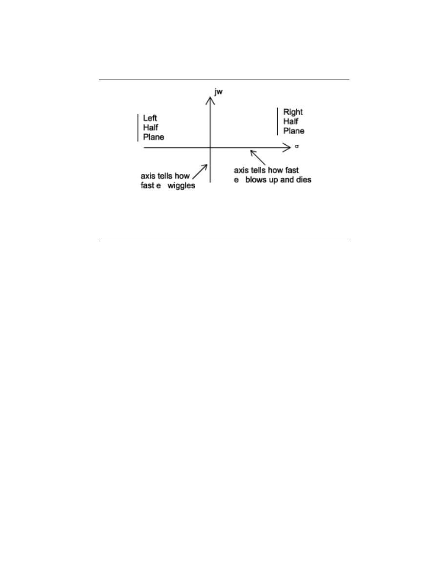
Figure 2.30:
This is the s-plane. Notice that any time s lies in the right half plane, the
complex exponential will grow through time, while any time it lies in the left half plane
it will decay.
Exercise 2.1:
What do the imaginary parts of the complex emponentials drawn above look like?
Solution:
They look the same except the oscillation is that of a sinusoid as opposed to a
cosinusoid (ie it passes through the origin rather than being a local maximum at
t = 0).
2.6.4 The Complex Plane
It becomes extremely useful to view the complex variable s as a point in the complex plane
(the s-plane ).
3.7 Discrete-Time Systems in the Time-Domain
A discrete-time signal s (n) is delayed by n
0
samples when we write s (n − n
0
), with n
0
> 0.
Choosing n
0
to be negative advances the signal along the integers. As opposed to analog
delays (pg ??), discrete-time delays can only be integer valued. In the frequency domain,
delaying a signal corresponds to a linear phase shift of the signal’s discrete-time Fourier
transform:
s (n − n
0
) ↔ e
−(j2πf n
0
)
S e
j2πf
.
Linear discrete-time systems have the superposition property.
S (a
1
x
1
(n) + a
2
x
2
(n)) = a
1
S (x
1
(n)) + a
2
S (x
2
(n))
(2.34)
A discrete-time system is called shift-invariant (analogous to time-invariant analog sys-
tems (pg ??)) if delaying the input delays the corresponding output.
If S (x (n)) = y (n), then
S (x (n − n
0
)) = y (n − n
0
)
(2.35)

34
CHAPTER 2. SIGNALS AND SYSTEMS: A FIRST LOOK
We use the term shift-invariant to emphasize that delays can only have integer values in
discrete-time, while in analog signals, delays can be arbitrarily valued.
We want to concentrate on systems that are both linear and shift-invariant. It will
be these that allow us the full power of frequency-domain analysis and implementations.
Because we have no physical constraints in ”constructing” such systems, we need only a
mathematical specification. In analog systems, the differential equation specifies the input-
output relationship in the time-domain. The corresponding discrete-time specification is
the difference equation .
y (n) = a
1
y (n − 1) + · · · + a
p
y (n − p) + b
0
x (n) + b
1
x (n − 1) + · · · + b
q
x (n − q)
(2.36)
Here, the output signal y (n) is related to its past values y (n − l), l = {1, . . . , p}, and
to the current and past values of the input signal x (n). The system’s characteristics are
determined by the choices for the number of coefficients p and q and the coefficients’ values
{a
1
, . . . , a
p
} and {b
0
, b
1
, . . . , b
q
}.
aside:
There is an asymmetry in the coefficients: where is a
0
? This coefficient
would multiply the y(n) term in Equation 2.36. We have essentially divided the
equation by it, which does not change the input-output relationship. We have thus
created the convention that a
0
is always one.
As opposed to differential equations, which only provide an implicit description of a
system (we must somehow solve the differential equation), difference equations provide an
explicit way of computing the output for any input.
We simply express the difference
equation by a program that calculates each output from the previous output values, and
the current and previous inputs.
Difference equations are usually expressed in software with for loops.
A MATLAB
program that would compute the first 1000 values of the output has the form
for n=1:1000
y(n) = sum(a.*y(n-1:-1:n-p)) + sum(b.*x(n:-1:n-q));
end
An important detail emerges when we consider making this program work; in fact, as
written it has (at least) two bugs. What input and output values enter into the computation
of y(1)? We need values for y(0), y(-1), ..., values we have not yet computed. To compute
them, we would need more previous values of the output, which we have not yet computed.
To compute these values, we would need even earlier values, ad infinitum. The way out
of this predicament is to specify the system’s initial conditions : we must provide the p
output values that occurred before the input started. These values can be arbitrary, but
the choice does impact how the system responds to a given input. One choice gives rise to a
linear system: Make the initial conditions zero. The reason lies in the definition of a linear
system: The only way that the output to a sum of signals can be the sum of the individual
outputs occurs when the initial conditions in each case are zero.
Exercise 2.2:
The initial condition issue resolves making sense of the difference equation for
inputs that start at some index. However, the program will not work because of a
programming, not conceptual, error. What is it? How can it be ”fixed?”
Solution:
The indices can be negative, and this condition is not allowed in MATLAB. To fix
it, we must start the signals later in the array.

35
Table 1
n
x(n)
y(n)
-1
0
0
0
1
b
1
0
ba
2
0
ba
2
:
0
:
n
0
ba
n
Figure 2.31
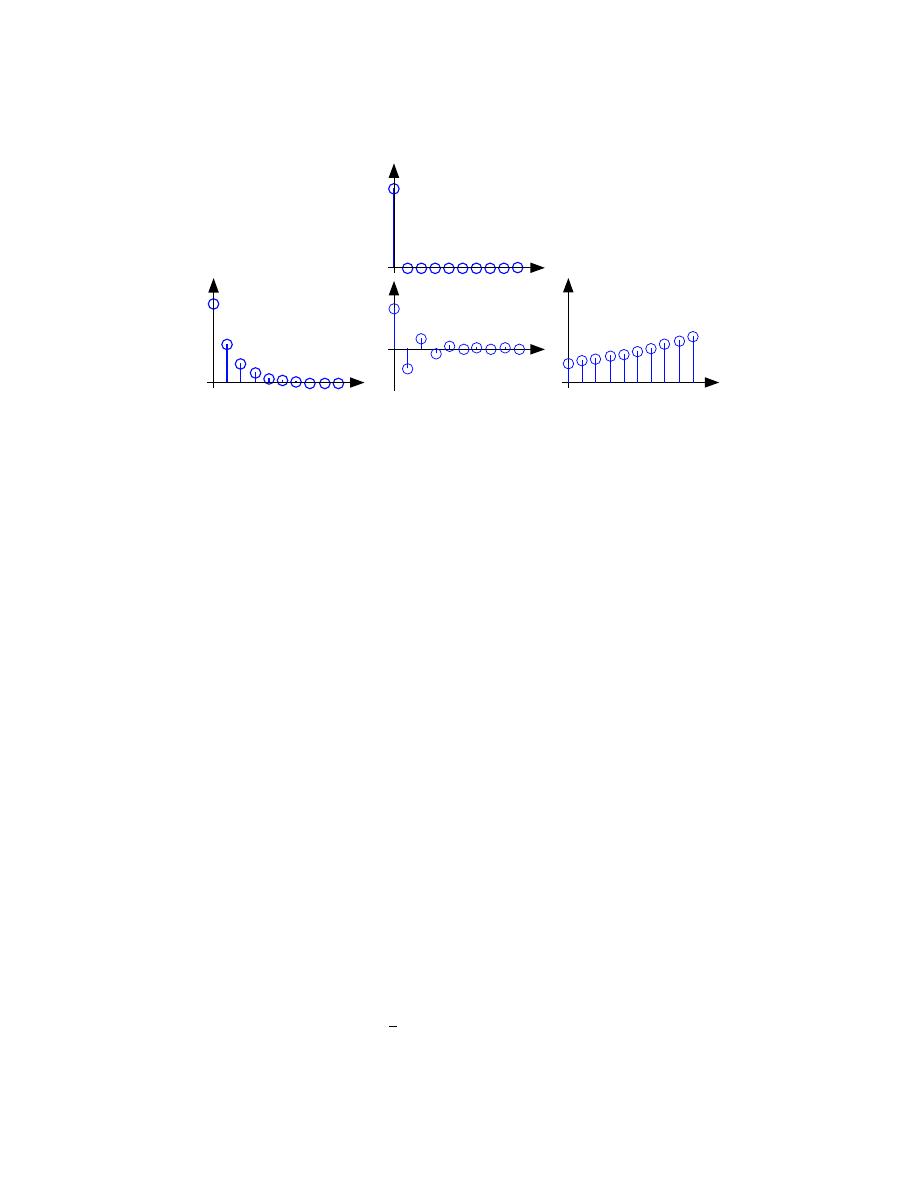
Example 2.2:
Let’s consider the simple system having p = 1 and q = 0.
y (n) = ay (n − 1) + bx (n)
(2.37)
To compute the output at some index, this difference equation says we need to know
what the previous output y (n − 1) and what the input signal is at that moment
of time. In more detail, let’s compute this system’s output to a unit-sample input:
x (n) = δ (n). Because the input is zero for negative indices, we start by trying to
compute the output at n = 0.
y (0) = ay (−1) + b
(2.38)
What is the value of y (−1)? Because we have used an input that is zero for all
negative indices, it is reasonable to assume that the output is also zero. Certainly,
the difference equation would not describe a linear system if the input that is zero
for all time did not produce a zero output. With this assumption, y (−1) = 0,
leaving y (0) = b. For n > 0, the input unit-sample is zero, which leaves us with
the difference equation ∀n, n > 0 : y (n) = ay (n − 1). We can envision how the
filter responds to this input by making a table.
y (n) = ay (n − 1) + bδ (n)
(2.39)
Coefficient values determine how the output behaves. The parameter b can be any
value, and serves as a gain. The effect of the parameter a is more complicated
(Figure 2.31). If it equals zero, the output simply equals the input times the gain
b. For all non-zero values of a, the output lasts forever; such systems are said to
be IIR ( I nfinite I mpulse Response). The reason for this terminology is that the
unit sample also known as the impulse (especially in analog situations), and the
system’s response to the ”impulse” lasts forever. If a is positive and less than one,
the output is a decaying exponential. When a = 1, the output is a unit step. If a is
negative and greater than −1, the output oscillates while decaying exponentially.
When a = 1, the output changes sign forever, alternating between b and −b. More
dramatic effects when |a| > 1; whether positive or negative, the output signal
becomes larger and larger, growing exponentially.
36
CHAPTER 2. SIGNALS AND SYSTEMS: A FIRST LOOK
1
n
y(n)
a = 0.5, b = 1
n
-1
1
y(n)
a = –0.5, b = 1
n
0
2
4
y(n)
a = 1.1, b = 1
x(n)
n
n
Figure 2.32:
The input to the simple example system, a unit sample, is shown at the
top, with the outputs for several system parameter values shown below.
Positive values of a are used in population models to describe how population size
increases over time. Here, n might correspond to generation. The difference equa-
tion says that the number in the next generation is some multiple of the previous
one. If this multiple is less than one, the population becomes extinct; if greater
than one, the population flourishes. The same difference equation also describes
the effect of compound interest on deposits. Here, n indexes the times at which
compounding occurs (daily, monthly, etc.), a equals the compound interest rate
plusone, and b = 1 (the bank provides no gain). In signal processing applications,
we typically require that the output remain bounded for any input. For our ex-
ample, that means that we restrict |a| = 1 and chose values for it and the gain
according to the application.
Exercise 2.3:
Note that the difference equation (Equation 2.36),
y (n) = a
1
y (n − 1) + · · · + a
p
y (n − p) + b
0
x (n) + b
1
x (n − 1) + · · · + b
q
x (n − q)
does not involve terms like y (n + 1) or x (n + 1) on the equation’s right side. Can
such terms also be included? Why or why not?
Solution:
Such terms would require the system to know what future input or output values
would be before the current value was computed. Thus, such terms can cause
difficulties.
Example 2.3:
A somewhat different system has no ”a” coefficients. Consider the difference equa-
tion
y (n) =
1
q
(x (n) + · · · + x (n − q + 1))
(2.40)
Because this system’s output depends only on current and previous input values, we
need not be concerned with initial conditions. When the input is a unit-sample,
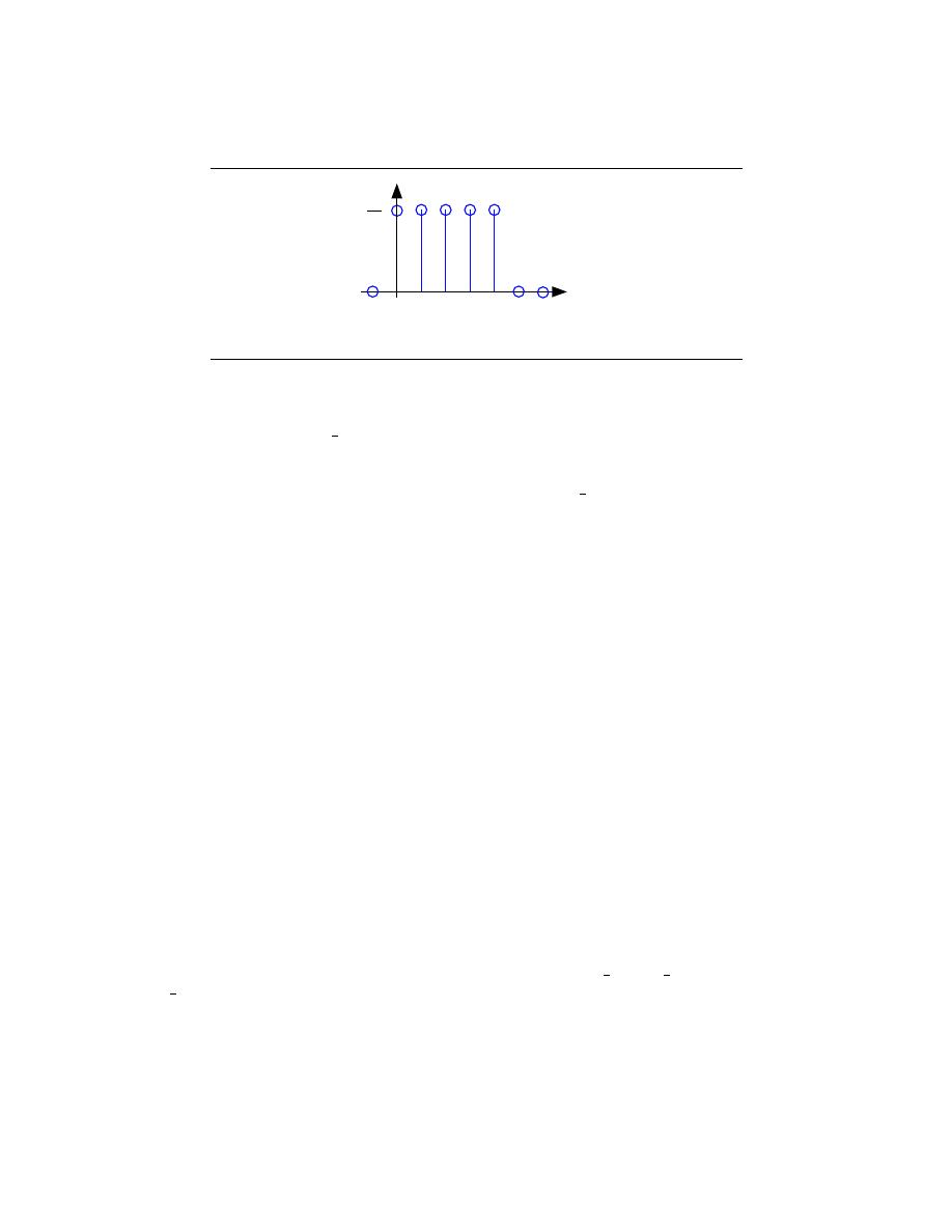
37
y(n)
n
1
5
Figure 2.33: The plot shows the unit-sample response of a length-5 boxcar filter.
the output equals
1
q
for n = {0, . . . , q − 1}, then equals zero thereafter. Such
systems are said to be FIR ( Finite I mpulse Response) because their unit sample
responses have finite duration. Plotting this response (Figure 2.33) shows that the
unit-sample response is a pulse of width q and height
1
q
. This waveform is also
known as a boxcar, hence the name boxcar filter given to this system. (We’ll
derive its frequency response and develop its filtering interpretation in the next
section.) For now, note that the difference equation says that each output value
equals the average of the input’s current and previous values. Thus, the output
equals the running average of input’s previous q values. Such a system could be
used to produce the average weekly temperature (q = 7) that could be updated
daily.
3.8 The Impulse Function
In engineering, we often deal with the idea of an action occuring at a point. Whether
it be a force at a point in space or a signal at a point in time, it becomes worth while to
develop some way of quantitatively defining this. This leads us to the idea of a unit impulse,
probably the second most important function, next to the complex exponential, in systems
and signals course.
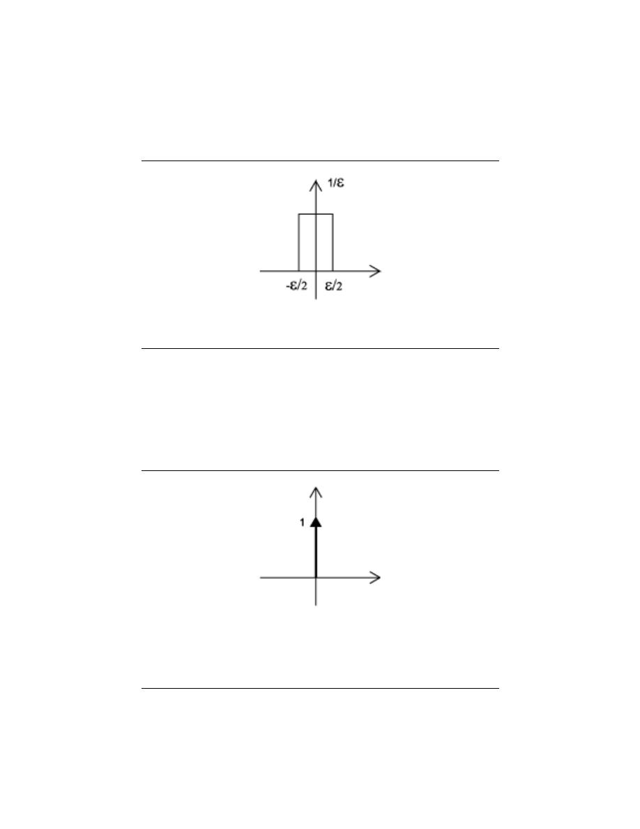
2.8.1 Dirac Delta Function
The Dirac Delta function , often referred to as the unit impulse or delta function, is the
function that defines the idea of a unit impulse. This function is one that is infinitesimally
narrow, infinitely tall, yet integrates to unity , one (see Equation 2.41 below). Perhaps the
simplest way to visualize this is as a rectangular pulse from a −
2
to a +
2
with a height of
1
. As we take the limit of this, lim
→0
0, we see that the width tends to zero and the height
tends to infinity as the total area remains constant at one. The impulse function is often
written as δ (t).
Z
∞
−∞
δ (t) dt = 1
(2.41)
38
CHAPTER 2. SIGNALS AND SYSTEMS: A FIRST LOOK
Figure 2.34:
This is one way to visualize the Dirac Delta Function.
Figure 2.35:
Since it is quite difficult to draw something that is infinitely tall, we
represent the Dirac with an arrow centered at the point it is applied. If we wish to scale
it, we may write the value it is scaled by next to the point of the arrow. This is a unit
impulse (no scaling).

39
2.8.1.1 The Sifting Property of the Impulse
The first step to understanding what this unit impulse function gives us is to examine what
happens when we multiply another function by it.
f (t) δ (t) = f (0) δ (t)
(2.42)
Since the impulse function is zero everywhere except the origin, we essentially just ”pick
off” the value of the function we are multiplying by evaluated at zero.
At first glance this may not appear to give use much, since we already know that the
impulse evaluated at zero is infinity, and anyhting times infinity is infinity. However, what
happens if we integrate this?
Sifting Property
R
∞
−∞
f (t) δ (t) dt
=
R
∞
−∞
f (0) δ (t) dt
=
f (0)
R
∞
−∞
δ (t) dt
=
f (0)
(2.43)
It quickly becomes apparent that what we end up with is simply the function evaluated at
zero. Had we used δ (t − T ) instead of δ (t), we could have ”sifted out” f (T ). This is what
we call the Sifting Property of the Dirac function, which is often used to define the unit
impulse.
The Sifting Property is very useful in developing the idea of convolution which is one
of the fundamental principles of signal processing. By using convolution and the sifting
property we can represent an approximation of any system’s output if we know the system’s
impulse response and input. Click on the convolution link above for more information on
this.
2.8.1.2 Other Impulse Properties
Below we will briefly list a few of the other properties of the unit impulse without going into
detail of their proofs - we will leave that up to you to verify as most are straightforward.
Note that these properties hold for continuous and discrete time.
Unit Impulse Properties
• - δ (αt) =
1
|α|
δ (t)
• - δ (t) = δ (−t)
• - δ (t) =
d
dt
u (t), where u (t) is the unit step.
2.8.2 Discrete-Time Impulse (Unit Sample)
The extension of the Unit Impulse Function to discrete-time becomes quite trivial. All we
really need to realize is that integration in continuous-time equates to summation in discrete-
time. Therefore, we are looking for a signal that sums to zero and is zero everywhere except
at zero.
Discrete-Time Impulse
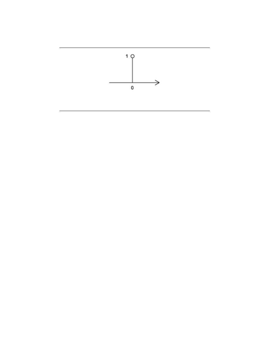
40
CHAPTER 2. SIGNALS AND SYSTEMS: A FIRST LOOK
Figure 2.36: The graphical representation of the discrete-time impulse function
δ [n] =
1 if n = 0
0 otherwise
(2.44)
Looking at the discrete-time plot of any discrete signal one can notice that all discrete
signals are composed of a set of scaled, time-shifted unit samples. If we let the value of a
sequence at each integer k be denoted by s [k] and the unit sample delayed that occurs at k
to be written as δ [n − k], we can write any signal as the sum of delayed unit samples that
are scaled by the signal value, or weighted coefficients.
s [n] =
∞
X
k=−∞
(s [k] δ [n − k])
(2.45)
This decomposition is strictly a property of discrete-time signals and proves to be a very
useful property.
note:
Through the above reasoning, we have formed Equation 2.45, which is the
fundamental concept of discrete-time convolution.
2.8.3 The Impulse Response
The impulse response is exactly what its name implies - the response of an LTI system,
such as a filter, when the system’s input is the unit impulse (or unit sample). A system
can be completed describe by its impulse response due to the idea mentioned above that
all signals can be represented by a superposition of signals. An impulse response gives an
equivalent description of a system as a transfer fucntion, since they are Laplace Transforms
of each other.
notation:
Most texts use δ (t) and δ [n] to denote the continuous-time and
discrte-time impulse response, respectively.
3.9 BIBO Stability
BIBO stands for bounded input, bounded output. BIBO stable is a condition such that any
bounded input yields a bounded output. This is to say that as long as we input a stable
signal, we are guaranteed to have a stable output.
In order to understand this concept, we must first look more closely into exactly what
we mean by bounded. A bounded signal is any signal such that there exists a value such
41
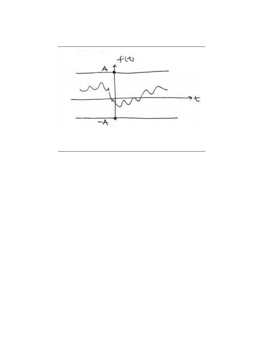
Figure 2.37:
A bounded signal is a signal for which there exists a constant A such that
∀t : |f (t) | < A
that the absolute value of the signal is never greater than some value. Since this value is
arbitrary, what we mean is that at no point can the signal tend to infinity.
Once we have identified what it means for a signal to be bounded, we must turn our
attention to the condition a system must posess in order to guarantee that if any bounded
signal is passed through the system, a bounded signal will arise on the output. It turns out
that a continuous-time LTI system with impulse response h (t) is BIBO stable if and only
if
Continuous-Time Condition for BIBO Stability
Z
∞
−∞
|h (t) |dt < ∞
(2.46)
This is to say that the transfer function is absolutely integrable.
To extend this concept to discrete-time, we make the standard transition from integration
to summation and get that the transfer function, h (n), must be absolutely summable. That
is
Discrete-Time Condition for BIBO Stability
∞
X
n=−∞
(|h (n) |) < ∞
(2.47)
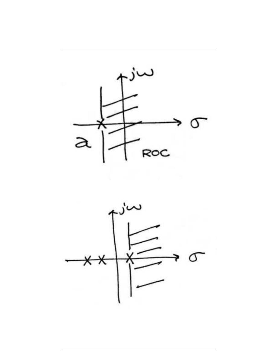
2.9.1 Stability and Laplace
Stability is very easy to infer from the pole-zero plot of a transfer function. The only
condition necessary to demonstrate stability is to show that the jω-axis is in the region of
convergence.
42
CHAPTER 2. SIGNALS AND SYSTEMS: A FIRST LOOK
(a)
(b)
Figure 2.38:
(a) Example of a pole-zero plot for a stable continuous-time system. (b)
Example of a pole-zero plot for an unstable continuous-time system.

43
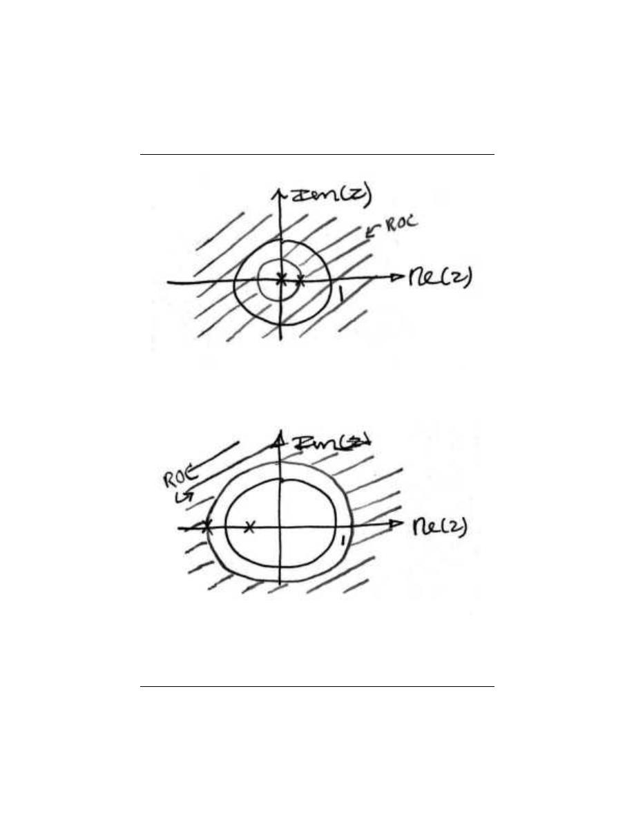
2.9.2 Stability and the Z-Transform
Stability for discrete-time signals in the z-domain is about as easy to demonstrate as it
is for continuous-time signals in the Laplace domain. However, instead of the region of
convergence needing to contain the jω-axis, the ROC must contain the unit circle.
44
CHAPTER 2. SIGNALS AND SYSTEMS: A FIRST LOOK
(a)
(b)
Figure 2.39:
(a) A stable discrete-time system. (b) An unstable discrete-time system.

Chapter 3
Time-Domain Analysis of CT
Systems
4.1 Systems in the Time-Domain
A discrete-time signal s (n) is delayed by n
0
samples when we write s (n − n
0
), with n
0
> 0.
Choosing n
0
to be negative advances the signal along the integers. As opposed to analog
delays (pg ??), discrete-time delays can only be integer valued. In the frequency domain,
delaying a signal corresponds to a linear phase shift of the signal’s discrete-time Fourier
transform: s (n − n
0
) ↔ e
−(j2πf n
0
)
S e
j2πf
.
Linear discrete-time systems have the superposition property.
Superposition
S (a
1
x
1
(n) + a
2
x
2
(n)) = a
1
S (x
1
(n)) + a
2
S (x
2
(n))
(3.1)
A discrete-time system is called shift-invariant (analogous to time-invariant analog sys-
tems (pg ??)) if delaying the input delays the corresponding output.
Shift-Invariant
If S (x (n)) = y (n) , T henS (x (n − n
0
)) = y (n − n
0
)
(3.2)
We use the term shift-invariant to emphasize that delays can only have integer values in
discrete-time, while in analog signals, delays can be arbitrarily valued.
We want to concentrate on systems that are both linear and shift-invariant. It will
be these that allow us the full power of frequency-domain analysis and implementations.
Because we have no physical constraints in ”constructing” such systems, we need only a
mathematical specification. In analog systems, the differential equation specifies the input-
output relationship in the time-domain. The corresponding discrete-time specification is
the difference equation .
The Difference Equation
y (n) = a
1
y (n − 1) + ... + a
p
y (n − p) + b
0
x (n) + b
1
x (n − 1) + ... + b
q
x (n − q)
(3.3)
Here, the output signal y (n) is related to its past values y (n − l), l = {1, ..., p}, and to the
current and past values of the input signal x (n). The system’s characteristics are determined
by the choices for the number of coefficients p and q and the coefficients’ values {a
1
, ..., a
p
}
and {b
0
, b
1
, ..., b
q
}.
45

46
CHAPTER 3. TIME-DOMAIN ANALYSIS OF CT SYSTEMS
aside:
There is an asymmetry in the coefficients: where is a
0
? This coefficient
would multiply the y (n) term in the difference equation (Equation 3.3). We have
essentially divided the equation by it, which does not change the input-output
relationship. We have thus created the convention that a
0
is always one.
As opposed to differential equations, which only provide an implicit description of a
system (we must somehow solve the differential equation), difference equations provide an
explicit way of computing the output for any input.
We simply express the difference
equation by a program that calculates each output from the previous output values, and
the current and previous inputs.
4.2 Continuous-Time Convolution
3.2.1 Motivation
Convolution helps to determine the effect a system has on an input signal. It can be shown
that a linear, time-invariant system is completely characterized by its impulse response.
At first glance, this may appear to be of little use, since impulse functions are not well
defnied in real applications. however, the sifting property of impulses (Section 2.8.1.1) tells
us that a signal can be decomposed into an infinite sum (integral) of scaled and shifted
impulses. By knowing how a system affects a single impulse, and by understanding the way
a signal is comprised of scaled and summed impulses, it seems reasonable that it should be
possible to scale and sum the impulse responses of a system in order to deteremine what
output signal will results from a particular input. This is precisely what convolution does -
convolution determines the system’s output from knowledge of the input and the system’s
impulse response.
In the rest of this module, we will examine exactly how convolution is defined from the
reasoning above. This will result in the convolution integral (see the next section) and its
properties. These concepts are very important in Electrical Engineering and will make any
engineer’s life a lot easier if the time is spent now to truly understand what is going on.
In order to fully understand convolution, you may find it useful to look at the discrete-
time convolution as well. It will also be helpful to experiment with the applets
1
available
on the internet. These resources will offer different approaches to this crucial concept.
3.2.2 Convolution Integral
As mentioned above, the convolution integral provides an easy mathematical way to express
the output of an LTI system based on an arbitrary signal, x (t), and the system’s impulse
response, h (t). The convolution integral is expressed as
y (t) =
Z
∞
−∞
x (τ ) h (t − τ ) dτ
(3.4)
Convolution is such an important tool that it is represented by the symbol *, and can be
written as
y (t) = (x (t) , h (t))
(3.5)
By making a simple change of variables into the convolution integral, τ = t − τ , we can
easily show that convolution is commutative :
(x (t) , h (t)) = (h (t) , x (t))
(3.6)
1
http://www.jhu.edu/∼signals

47
Figure 3.1:
We begin with a system defined by its impulse response, h (t).
For more information on the characteristics of the convolution integral, read about the
Properties of Convolution.
We now present two distinct approaches for deriving the vonvolution integral. These
derivations, along with a basic example, will help to build intuition about convolution.
3.2.3 Derivation I: The Short Approach
The derivation used here closely follows the one discussed in the Motivation (Section 3.2.1)
section above. To begin this, it is necessary to state the assumptions we will be making. In
this instance, the only constraints on our system are that it be linear and time-invariant.
Brief Overview of Derivation Steps:
1. - An impulse input leads to an impulse response output.
2. - A shifted imulse input leads to a shifted impulse response output. This is due to the
time-invariance of the system.
3. - We now scale the impulse input to get a scaled impulse output. This is using the
scalar multiplication property of linearity.
4. - We can now ”sum up” an infinite number of these scaled impulses to get a sum of
an infinite number of scaled impulse responses. This is using the additivity attribute
of linearity.
5. - Now we recognize that this infinite sum is nothing more than an integral, so we
convert both sides into integrals.
6. - Recognizing that the input is the function f (t), we also recognize that the output is
exactly the convolution integral.
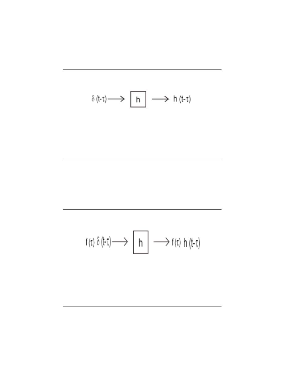
48
CHAPTER 3. TIME-DOMAIN ANALYSIS OF CT SYSTEMS
Figure 3.2:
We then consider a shifted version of the input impulse. Due to the time
invariance of the system, we obtain a shifted version of the output impulse response.
Figure 3.3:
Now we use the scaling part of linearity by scaling the system by a value,
f (τ ), that is constant with respect to the system variable, t.
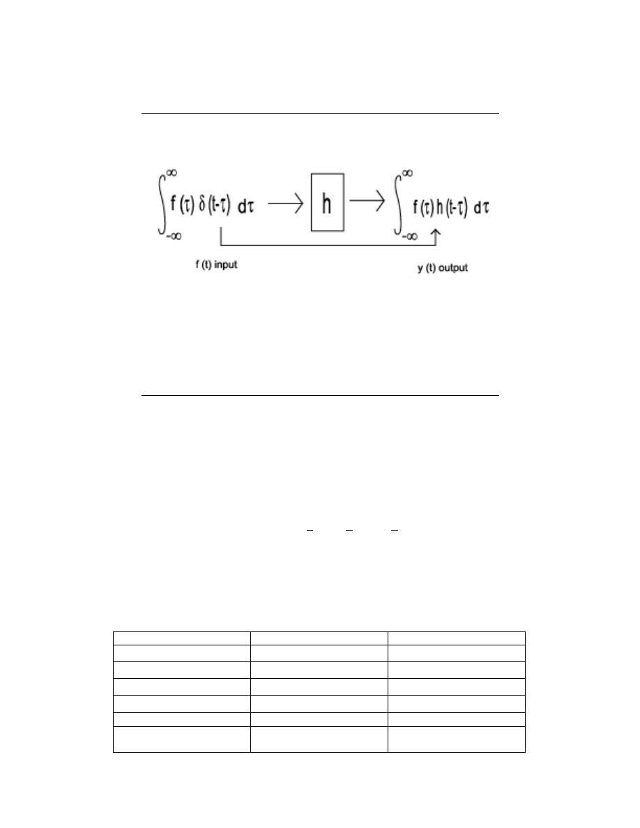
49
Figure 3.4:
We can now use the additivity aspect of linearity to add an infinite number
of these, one for each possible τ . Since an infinite sum is exactly an integral, we end up
with the integration known as the Convolution Integral. Using the sifting property, we
recognize the left-hand side simply as the input f (t).
3.2.4 Derivation II: The Long Approach
This derivation is really not too different from the one above. It is, however, a little more
rigorous and a little longer. Hopefully, if you think you ”kind of” get the derivation above,
this will help you gain a more complete understanding of convolution.
The first step in this derivation is to define a particular realization of the unit impulse
function. For this, we will use δ
∆
(t) =
1
∆
if −
∆
2
< t <
∆
2
0 otherwise
After defining our realization of the unit impulse response, we can derive our convolution
intergral from the following steps found in the table below. Note that the left column
represents the input and the right column is the system’s output given that input.
Derivation II of Convolution Integral
Input
Output
lim
∆→0
δ
∆
(t)
→ h →
lim
∆→0
h (t)
lim
∆→0
δ
∆
(t − n∆)
→ h →
lim
∆→0
h (t − n∆)
lim
∆→0
f (n∆) δ
∆
(t − n∆) ∆
→ h →
lim
∆→0
f (n∆) h (t − n∆) ∆
lim
∆→0
P
n
(f (n∆) δ
∆
(t − n∆) ∆)
→ h →
lim
∆→0
P
n
(f (n∆) h (t − n∆) ∆)
R
∞
−∞
f (τ ) δ (t − τ ) dτ
→ h →
R
∞
−∞
f (τ ) h (t − τ ) dτ
f (t)
→ h →
y (t)
=
R
∞
−∞
f (τ ) h (t − τ ) dτ
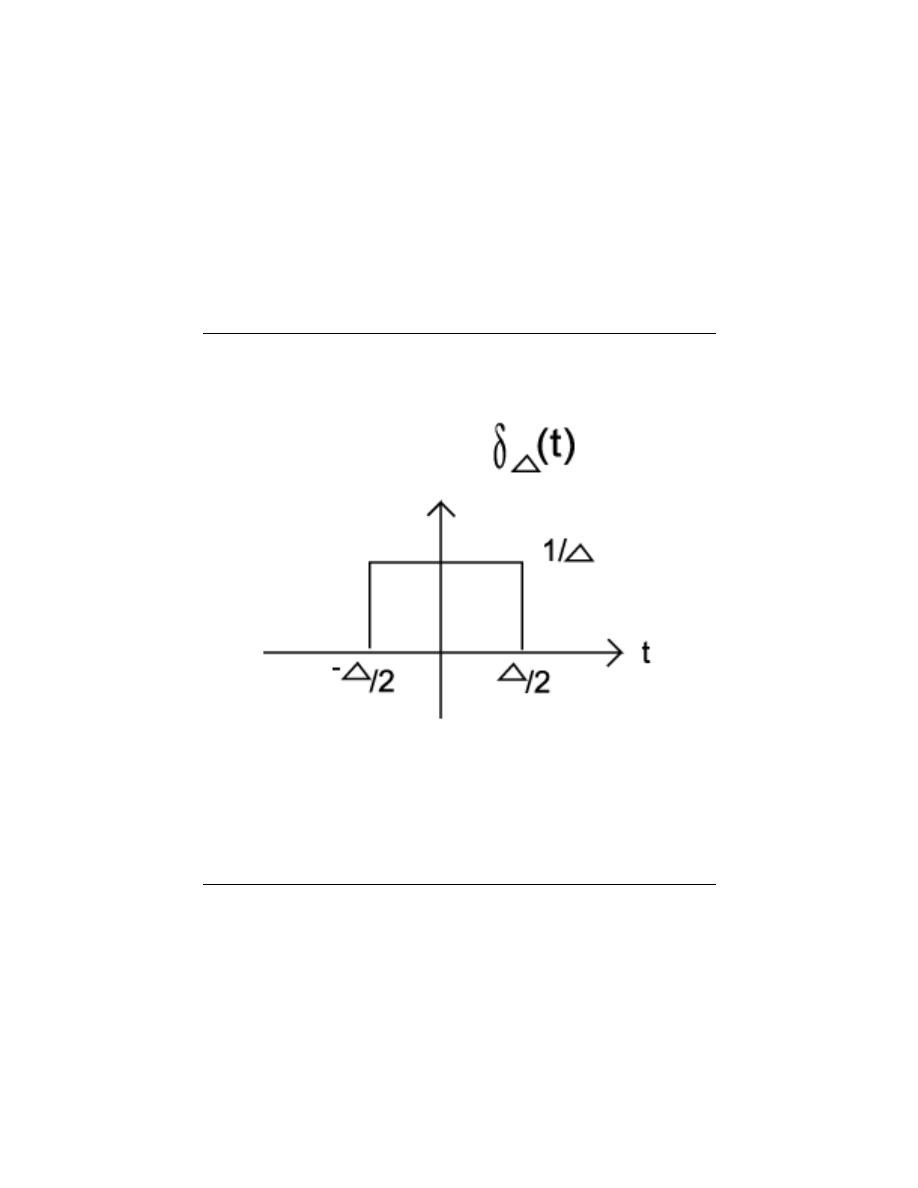
50
CHAPTER 3. TIME-DOMAIN ANALYSIS OF CT SYSTEMS
Figure 3.5:
The realization of the unit impulse function that we will use for this
example.
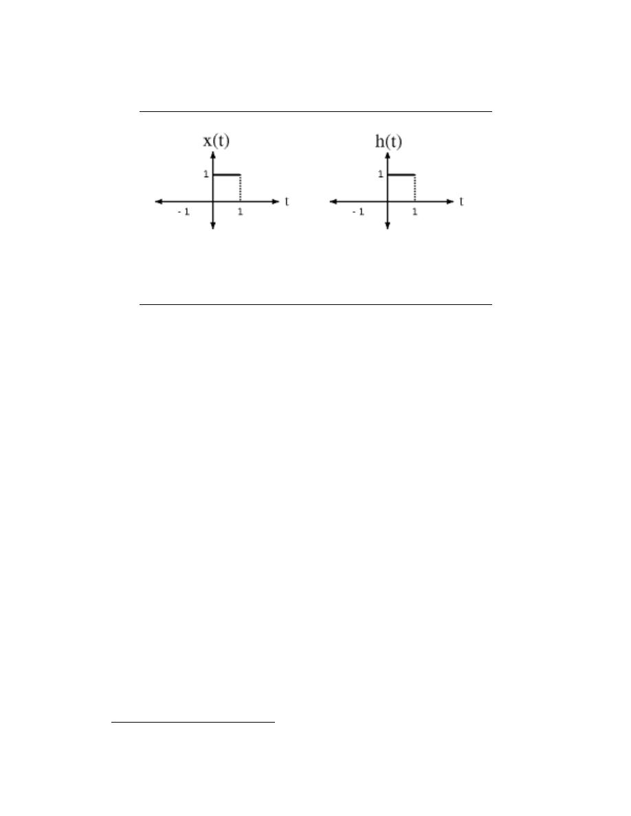
51
(a)
(b)
Figure 3.6:
Here are the two basic signals that we will convolve together.
3.2.5 Implementation of Convolution
Taking a closer look at the convolution integral, we find that we are multiplying the input
signal by the time-reversed impulse response and integrating. This will give us the value
of the output at one given value of t. If we then shift the time-reversed impulse response
by a small amount, we get the output for another value of t. Repeating this for every
possible value of t, yields the total output function. While we would never actually do
this computation by hand in this fashion, it does provide us with some insight into what is
actually happening. We find that we are essentially reversing the impulse response function
and sliding it across the input function, integrating as we go. This method, referred to as the
graphical method , provides us with a much simpler way to solve for the output for simple
(contrived) signals, while improving our intuition for the more complex cases where we rely
on computers. In fact Texas Instruments
2
developes Digital Signal Processors
3
which have
special instruction sets for computations such as convolution.
3.2.6 Basic Example
Let us look at a basic continuous-time convolution example to help express some of the ideas
mentioned above through a short example. We will convolve together two unit pulses, x (T )
and h (T ).
3.2.6.1 Reflect and Shift
Now we will take one of the functions and reflect it around the y-axis. Then we must shift
the function, such that the origin, the point of the function that was originally on the origin,
is labeled as point t. This step is shown in the figure below, h (t − T ). Since convolution
is commutative it will never matter which function is reflected and shifted; however, as the
functions become more complicated reflecting and shifting the ”right one” will often make
the problem much easier.
2
http://www.ti.com
3
http://dspvillage.ti.com/docs/toolssoftwarehome.jhtml
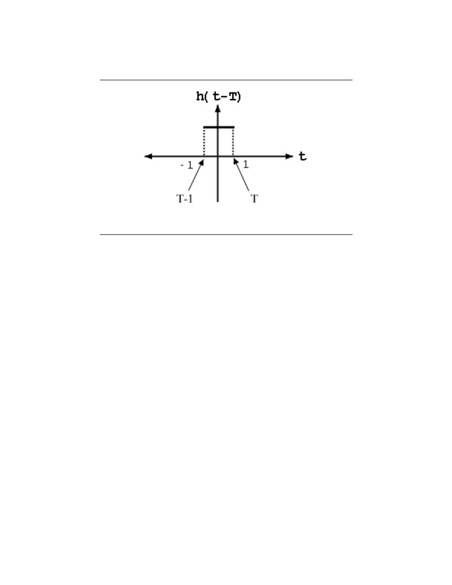
52
CHAPTER 3. TIME-DOMAIN ANALYSIS OF CT SYSTEMS
Figure 3.7:
The reflected and shifted unit pulse.
3.2.6.2 Regions of Integration
Next, we want to look at the functions and divide the span of the functions into different
limits of integration. These different regions can be understood by thinking about how
we slide h (t − T ) over the other function. These limits come from the different regions of
overlap that occur between the two functions. If the function were more complex, then
we would need to have more limits so that that overlapping parts of both function could
be expressed in a single, linear integral. For this problem we will have the following four
regions. Compare these limits of integration to the sketches of h (t − T ) and x (T ) to see if
you can understand why we have the four regions. Note that the t in the limits of integration
refers to the right-hand side of h (t − T )’s function, labeled as t between zero and one on
the plot.
Four Limits of Integration
1. - t < 0
2. - 0 ≤ t < 1
3. - 1 ≤ t < 2
4. - t ≥ 2
3.2.6.3 Using the Convolution Integral
Finally we are ready for a little math. Using the convolution integral, let us integrate the
product of x (T ) h (t − T ). For our first and fourth region this will be trivial as it will always
be 0. The second region, 0 ≤ t < 1, will require the following math:
y (t)
=
R
t
0
1dT
=
t
(3.7)
The third region, 1 ≤ t < 2, is solved in much the same manner. Take note of the changes
in our integration though. As we move h (t − T ) across our other function, the left-hand
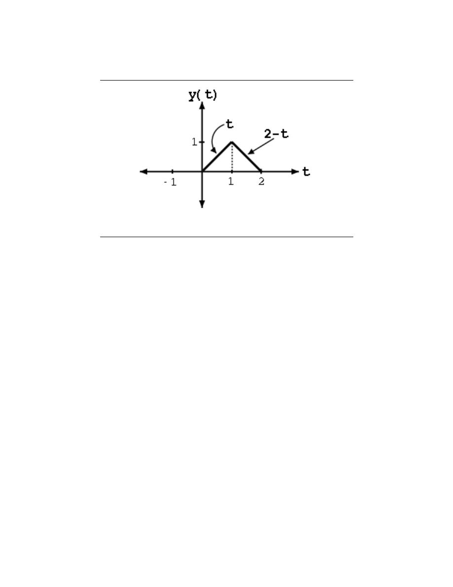
53
Figure 3.8:
Shows the system’s response to the input, x (t).
edge of the function, t − 1, becomes our lowlimit for the integral. This is shown through
our convolution integral as
y (t)
=
R
1
t−1
1dT
=
1 − (t − 1)
=
2 − t
(3.8)
The above formulas show the method for calculating convolution; however, do not let the
simplicity of this example confuse you when you work on other problems. The method will
be the same, you will just have to deal with more math in more complicated integrals.
3.2.6.4 Convolution Results
Thus, we have the following results for our four regions:
y (t) =
0 if t < 0
t if 0 ≤ t < 1
2 − t if 1 ≤ t < 2
0 if t ≥ 2
(3.9)
Now that we have found the resulting function for each of the four regions, we can combine
them together and graph the convolution of (x (t) , h (t)).
4.3 Properties of Convolution
In this module we will look at several of the most prevalent properties of convolution. Note
that these properties aply to both continuous-time convolution and discrete-time convolu-
tion. (Refer back to these two modules if you need a review of convolution). Also, for the
proofs of some of the properties, we will be using continuous-time integrals, but we could
prove them the same way using the discrete-time summations.
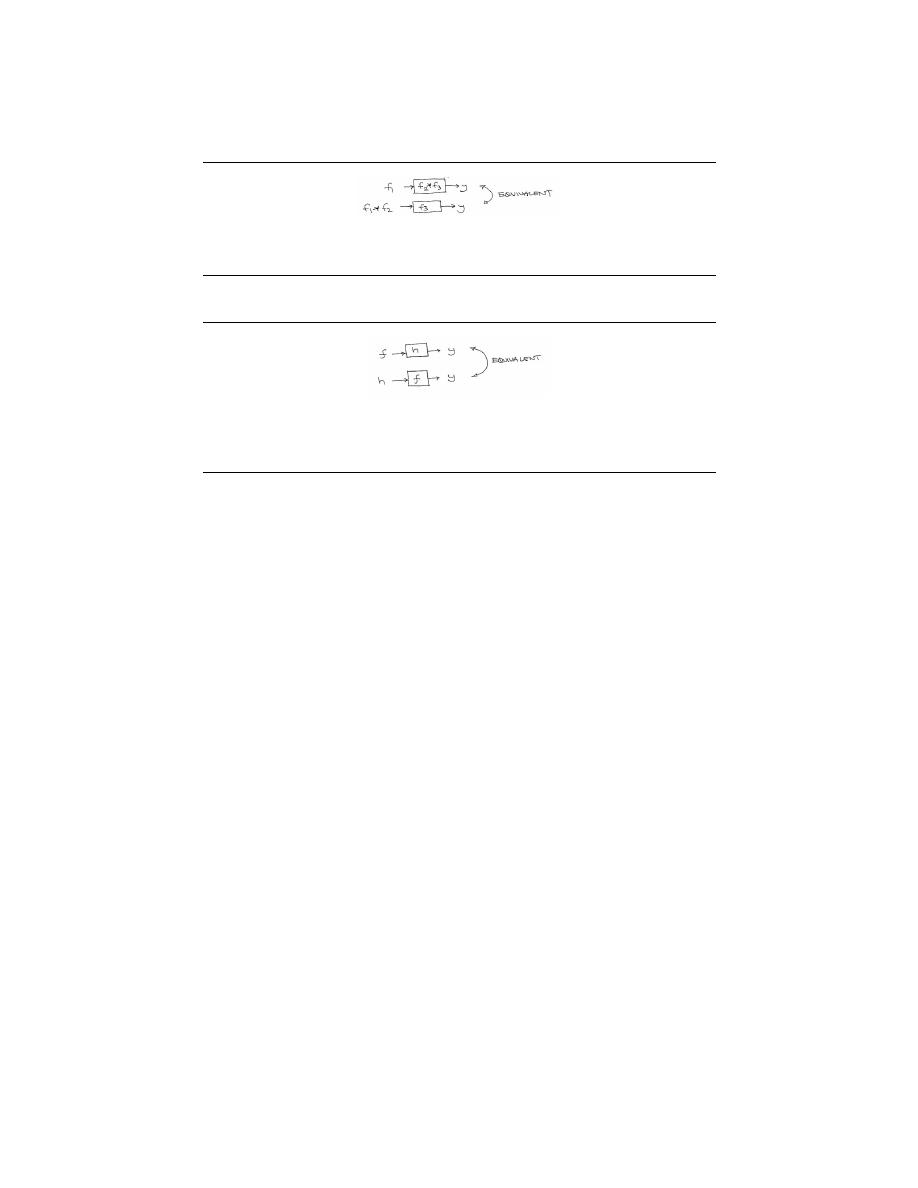
54
CHAPTER 3. TIME-DOMAIN ANALYSIS OF CT SYSTEMS
Figure 3.9:
Graphical implication of the associative property of convolution.
Figure 3.10:
The figure shows that either function can be regarded as the system’s
input while the other is the impulse response.
3.3.1 Associativity
Theorem 3.1:
Associative Law
(f
1
(t) , (f
2
(t) , f
3
(t))) = ((f
1
(t) , f
2
(t)) , f
3
(t))
(3.10)
3.3.2 Commutativity
Theorem 3.2:
Commutative Law
y (t)
=
(f (t) , h (t))
=
(h (t) , f (t))
(3.11)
Proof:
To prove Equation 3.11, all we need to do is make a simple change of variables in
our convolution integral (or sum),
y (t) =
Z
∞
−∞
f (τ ) h (t − τ ) dτ
(3.12)
By letting τ = t − τ , we can easily show that convolution is commutative :
y (t)
=
R
∞
−∞
f (t − τ ) h (τ ) dτ
=
R
∞
−∞
h (τ ) f (t − τ ) dτ
(3.13)
(f (t) , h (t)) = (h (t) , f (t))
(3.14)

55
Figure 3.11
3.3.3 Distribution
Theorem 3.3:
Distributive Law
(f
1
(t) , f
2
(t) + f
3
(t)) = (f
1
(t) , f
2
(t)) + (f
1
(t) , f
3
(t))
(3.15)
Proof:
The proof of this theorem can be taken directly from the definition of convolution
and by using the linearity of the integral.
3.3.4 Time Shift
Theorem 3.4:
Shift Property
For c (t) = (f (t) , h (t)), then
c (t − T ) = (f (t − T ) , h (t))
(3.16)
and
c (t − T ) = (f (t) , h (t − T ))
(3.17)
3.3.5 Convolution with an Impulse
Theorem 3.5:
Convolving with Unit Impulse
(f (t) , δ (t)) = f (t)
(3.18)
Proof:
For this proof, we will let δ (t) be the unit impulse located at the origin. Using the
definition of convolution we start with the convolution integral
(f (t) , δ (t)) =
Z
∞
−∞
δ (τ ) f (t − τ ) dτ
(3.19)
From the definition of the unit impulse, we know that δ (τ ) = 0 whenever τ 6= 0.
We use this fact to reduce the above equation to the following:
(f (t) , δ (t))
=
R
∞
−∞
δ (τ ) f (t) dτ
=
f (t)
R
∞
−∞
(δ (τ )) dτ
(3.20)
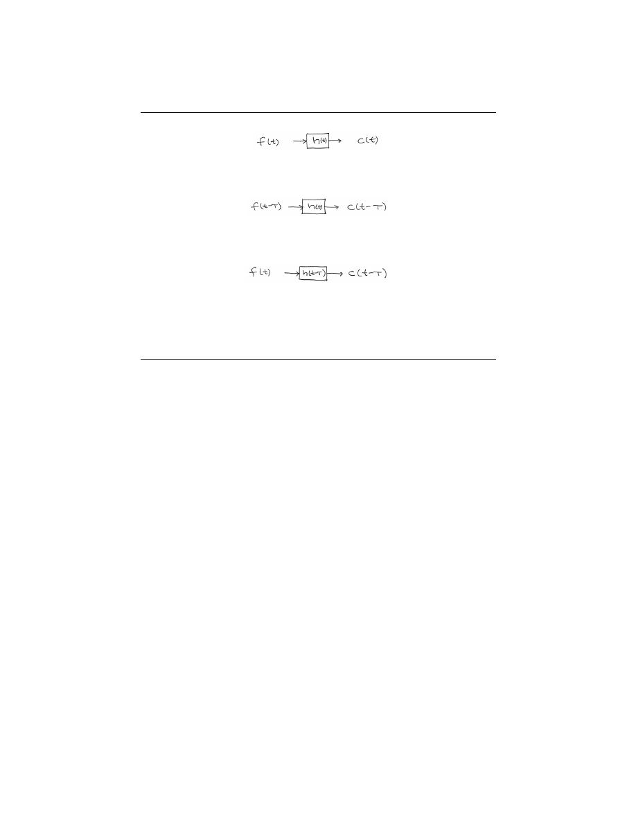
56
CHAPTER 3. TIME-DOMAIN ANALYSIS OF CT SYSTEMS
(a)
(b)
(c)
Figure 3.12:
Graphical demonstration of the shift property.
The integral of δ (τ ) will only have a value when τ = 0 (from the definition of
the unit impulse), therefore its integral will equal one. Thus we can simplify the
equation to our theorem:
(f (t) , δ (t)) = f (t)
(3.21)
3.3.6 Width
If Duration (f
1
) = T
1
and Duration (f
2
) = T
2
, then
Duration ((f
1
, f
2
)) = T
1
+ T
2
(3.22)
3.3.7 Causality
If f and h are both causal, then (f, h) is also causal.
4.4 Discrete-Time Convolution
3.4.1 Overview
Convolution is a concept that extends to all systems that are both linear and time-
invariant (LTI ). The idea of discrete-time convolution is exactly the same as that
of continuous-time convolution. For this reason, it may be useful to look at both versions
to help your understanding of this extremely important concept. Recall that convolution is
a very powerful tool in determining a system’s output from knowledge of an arbitrary input
and the system’s impulse response. It will also be helpful to see convolution graphically with

57
(a)
(b)
Figure 3.13:
The figures, and equation above, reveal the identity function of the unit
impulse.
(a)
(b)
(c)
Figure 3.14:
From the images, you can see that the length, or duration, of the resulting
signal after convolution will be equal to the sum of the lengths of each of the individual
signals be convolved.

58
CHAPTER 3. TIME-DOMAIN ANALYSIS OF CT SYSTEMS
your own eyes and to play around with it some, so experiment with the applets
4
available
on the internet. These resources will offer different approaches to this crucial concept.
3.4.2 Convolution Sum
As mentioned above, the convolution sum provides a concise, mathematical way to express
the output of an LTI system based on an arbitrary discrete-time input signal and the system’s
response. The convolution sum is expressed as
y [n] =
∞
X
k=−∞
(x [k] h [n − k])
(3.23)
As with continuous-time, convolution is represented by the symbol *, and can be written as
y [t] = x [t] ∗ h [t]
(3.24)
By making a simple change of variables into the convolution sum, k = n − k, we can easily
show that convolution is commutative :
x [t] ∗ h [t] = h [t] ∗ x [t]
(3.25)
For more information on the characteristics of convolution, read about the Properties of
Convolution.
3.4.3 Derivation
We know that any discrete-time signal can be represented by a summation of scaled and
shifted discrete-time impulses. Since we are assuming the system to be linear and time-
invariant, it would seem to reason that an input signal comprised of the sum of scaled and
shifted impulses would give rise to an output comprised of a sum of scaled and shifted
impulse responses. This is exactly what occurs in convolution . Below we present a more
rigorous and mathematical look at the derivation:
Letting H be a DT LTI system, we start with the folowing equation and work our way
down the the convoluation sum!
y [n]
=
H [x [n]]
=
H
P
∞
k=−∞
(x [k] δ [n − k])
=
P
∞
k=−∞
(H [x [k] δ [n − k]])
=
P
∞
k=−∞
(x [k] H [δ [n − k]])
=
P
∞
k=−∞
(x [k] h [n − k])
(3.26)
Let us take a quick look at the steps taken in the above derivation. After our initial equation,
we using the DT sifting property (Section 2.8.1.1) to rewrite the function, x [n], as a sum
of the function times the unit impulse. Next, we can move around the H operator and the
summation because H [@] is a linear, DT system. Because of this linearity and the fact that
x [k] is a constannt, we can pull the previous mentioned constant out and simply multiply
it by H [@]. Finally, we use the fact that H [@] is time invariant in order to reach our final
state - the convolution sum!
A quick graphical example may help in demonstrating why convolution works.
4
http://www.jhu.edu/∼signals
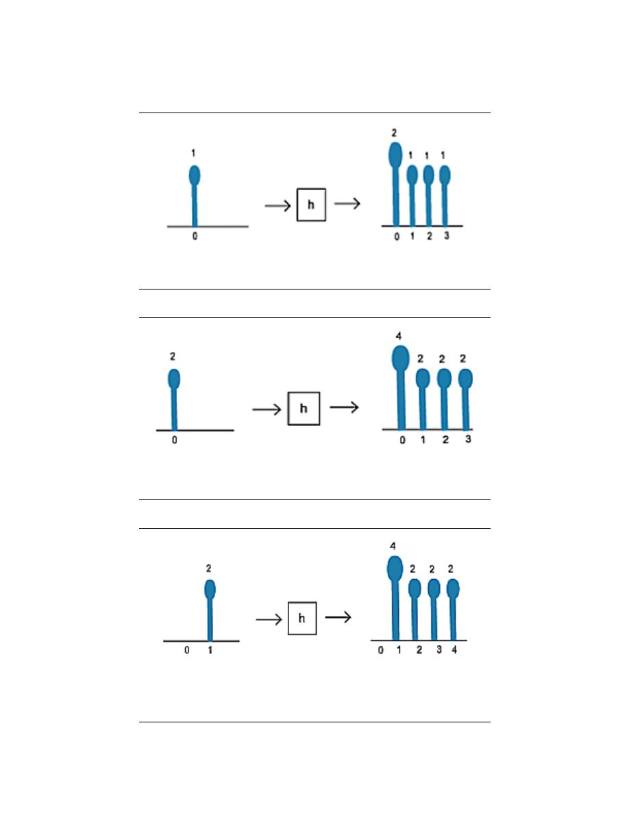
59
Figure 3.15:
A single impulse input yields the system’s impulse response.
Figure 3.16:
A scaled impulse input yields a scaled response, due to the scaling
property of the system’s linearity.
Figure 3.17:
We now use the time-invariance property of the system to show that a
delayed input results in an output of the same shape, only delayed by the same amount
as the input.
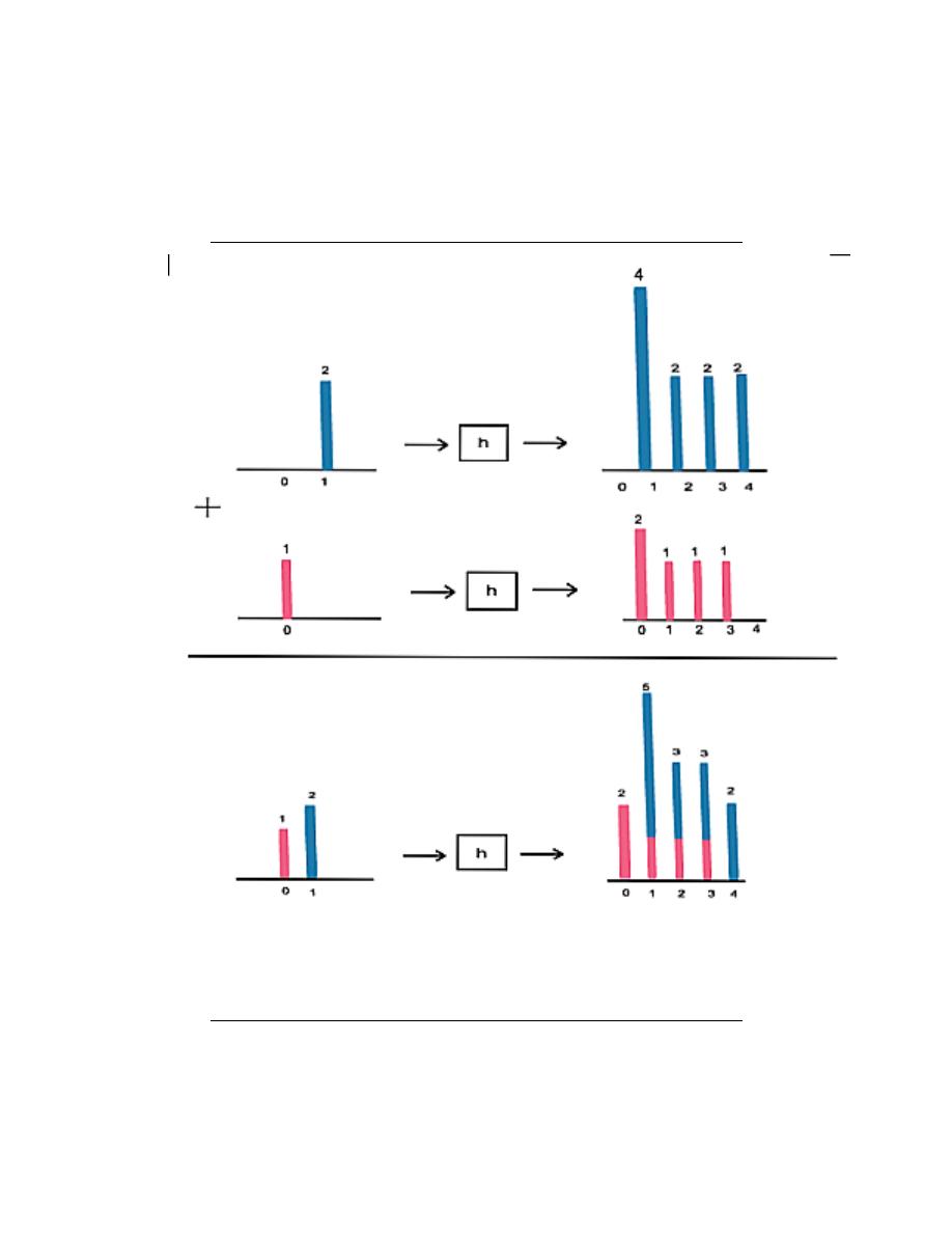
60
CHAPTER 3. TIME-DOMAIN ANALYSIS OF CT SYSTEMS
Figure 3.18:
We now use the additivity portion of the linearity property of the system
to complete the picture. Since any discrete-time signal is just a sum of scaled and shifted
discrete-time impulses, we can find the output from knowing the input and the impulse
response.
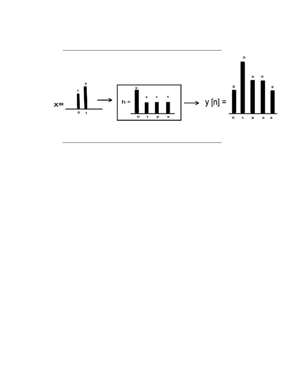
61
Figure 3.19:
This is the end result that we are looking to find.
3.4.4 Convolution Through Time (A Graphical Approach)
In this section we will develop a second graphical interpretation of discrete-time convolution.
We will begin this by writing the convolution sum allowing x to be a causal, length-m signal
and h to be a causal, length-k, LTI system. This gives us the finite summation,
y [l] =
m
X
l=0
(x [l] h [n − l])
(3.27)
Notice that for any given n we have a sum of the products of x
l
and a time-delayed h
−l
.
This is to say that we multiply the terms of x by the terms of a time-reversed h and add
them up.
Going back to the previous example:
What we are doing in the above demonstration is reversing the impulse response in time
and ”walking it across” the input signal. Clearly, this yields the same result as scaling,
shifting and summing impulse responses.
This approach of time-reversing, and sliding across is a common approach to presenting
convolution, since it demonstrates how convolution builds up an output through time.
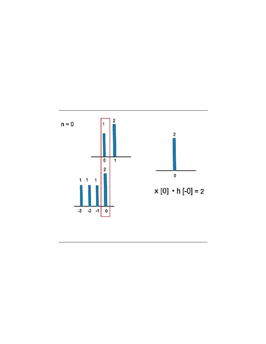
62
CHAPTER 3. TIME-DOMAIN ANALYSIS OF CT SYSTEMS
Figure 3.20:
Here we reverse the impulse response, h , and begin its traverse at time
0.
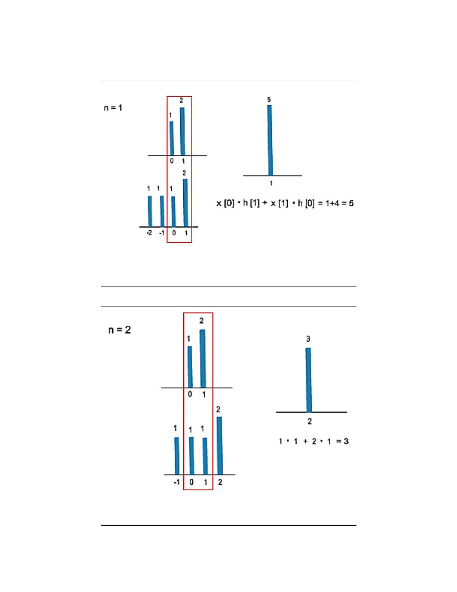
63
Figure 3.21:
We continue the traverse. See that at time 1 , we are multiplying two
elements of the input signal by two elements of the impulse respone.
Figure 3.22
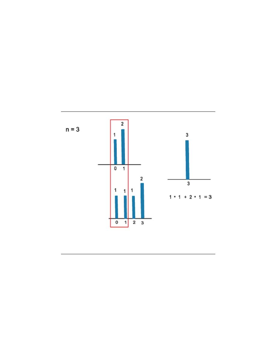
64
CHAPTER 3. TIME-DOMAIN ANALYSIS OF CT SYSTEMS
Figure 3.23:
If we follow this through to one more step, n = 4, then we can see that
we produce the same output as we saw in the intial example.

Chapter 4
Linear Algebra Overview
5.1 Linear Algebra: The Basics
This brief tutorial on some key terms in linear algebra is not meant to replace or be very
helpful to those of you trying to gain a deep insight into linear algebra.
Rather, this
brief introduction to some of the terms and ideas of linear algebra is meant to provide a
little background to those trying to get a better understanding or learn about eigenvectors
and eigenfunctions, which play a big role in deriving a few important ideas on Signals and
Systems. The goal of these concepts will be to provide a background for signal decomposition
and to lead up to the derivation of the Fourier Series.
4.1.1 Linear Independence
A set of vectors ∀x, x
i
∈ C
n
: {x
1
, x
2
, . . . , x
k
} are linearly independent if none of them
can be written as a linear combination of the others.
Linearly Independent :
For a given set of vectors, {x
1
, x
2
, . . . , x
n
}, they are
linearly independent if
c
1
x
1
+ c
2
x
2
+ · · · + c
n
x
n
= 0
only when c
1
= c
2
= · · · = c
n
= 0
Example 4:
We are given the following two vectors:
x
1
=
3
2
x
2
=
−6
−4
These are not linearly independent as proven by the following statement,
which, by inspection, can be seen to not adhere to the definition of linear
independence stated above.
x
2
= −2x
1
⇒ 2x
1
+ x
2
= 0
Another approach to reveal a vectors indendence is by graphing the vec-
tors. Looking at these two vectors geometrically (as in the figure below),
one can again prove that these vectors are not linearly independent.
65
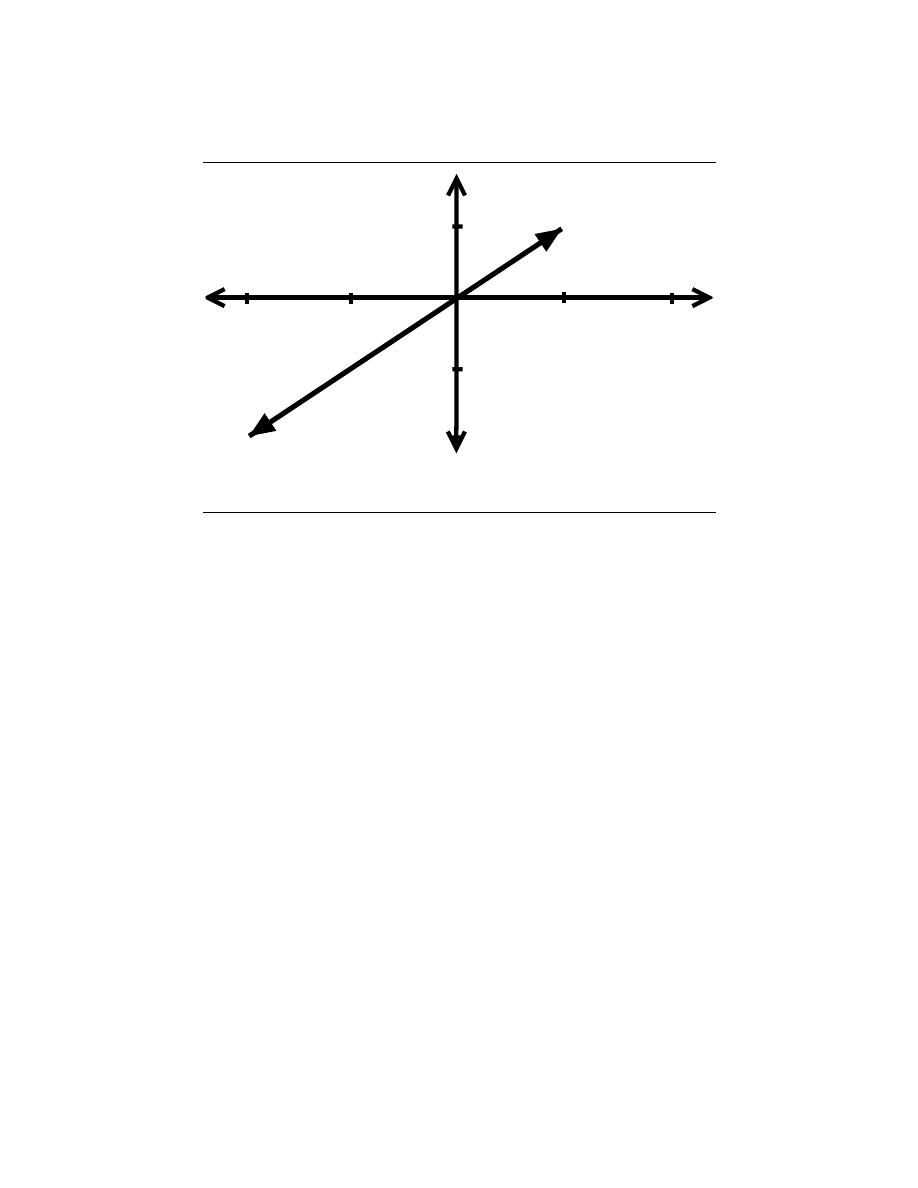
66
CHAPTER 4. LINEAR ALGEBRA OVERVIEW
3
-6
2
4
Figure 4.1:
Graphical representation of two vectors that are not linearly independent.
Example 4.1:
We are given the following two vectors:
x
1
=
3
2
x
2
=
1
2
These are linearly independent since
c
1
x
1
= − (c
2
x
2
)
only if c
1
= c
2
= 0. Based on the definition, this proof shows that these vectors
are indeed linearly independent. Again, we could also graph these two vectors (see
the figure below) to check for linear independence.
Exercise 4.1:
Are {x
1
, x
2
, x
3
} linearly independent?
x
1
=
3
2
x
2
=
1
2
x
3
=
−1
0
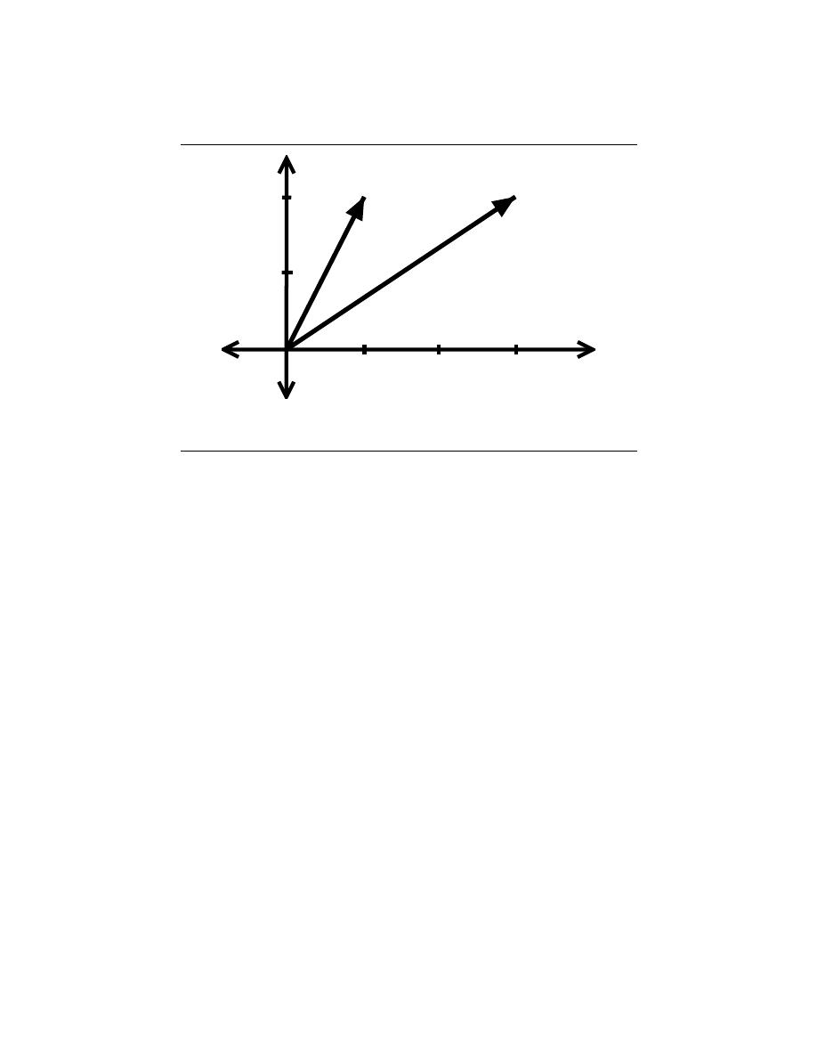
67
3
2
1
Figure 4.2:
Graphical representation of two vectors that are linearly independent.
Solution:
By playing around with the vectors and doing a little trial and error, we will
discover the following relationship:
x
1
− x
2
+ 2x
3
= 0
Thus we have found a linear combination of these three vectors that equals zero
without setting the coefficients equal to zero. Therefore, these vectors are not
linearly independent!
As we have seen in the two above examples, often times the independence of vectors can
be easily seen through a graph. However this may not be as easy when we are given three
or more vectors. Can you easily tell whether or not these vectors are independent from the
figure below. Probably not, which is why the method used in the above solution becomes
important.
hint:
A set of m vectors in C
n
cannot be linearly independent if m > n.
4.1.2 Span
Span :
The span (pg ??) of a set of vectors {x
1
, x
2
, . . . , x
k
} is the set of vectors
that can be written as a linear combination of {x
1
, x
2
, . . . , x
k
}
span ({x
1
, . . . , x
k
}) = {∀α, α
i
∈ C
n
: α
1
x
1
+ α
2
x
2
+ · · · + α
k
x
k
}
Example 6:
Given the vector
x
1
=
3
2
the span of x
1
is a line.
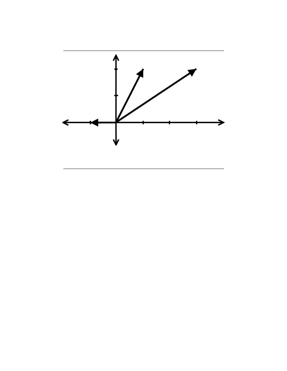
68
CHAPTER 4. LINEAR ALGEBRA OVERVIEW
3
2
1
-1
Figure 4.3:
Plot of the three vectors. Can be shown that a linear combination exists
among the three, and therefore they are not linear independent.
Example 7:
Given the vectors
x
1
=
3
2
x
2
=
1
2
the span of these vectors is C
2
.
4.1.3 Basis
Basis :
A basis for C
n
is a set of vectors that: (1) spans C
n
and (2) is linearly
independent.
Clearly, any set of n linearly independent vectors is a basis for C
n
.
Example 4.2:
We are given the following vector
e
i
=
0
..
.
0
1
0
..
.
0
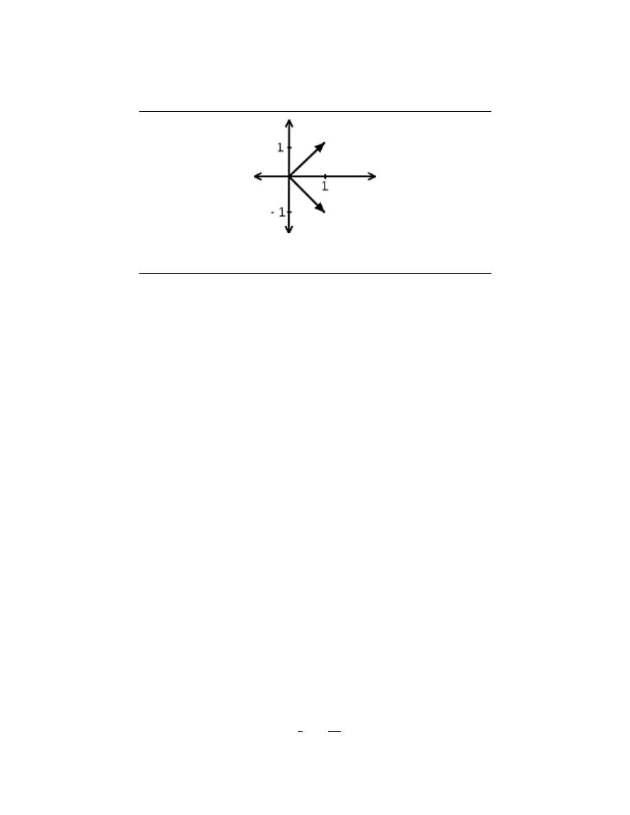
69
Figure 4.4:
Plot of basis for C
2
where the 1 is always in the ith place and the remaining values are zero. Then the
basis for C
n
is
{∀i, i = [1, 2, . . . , n] : e
i
}
note:
{∀i, i = [1, 2, . . . , n] : e
i
} is called the ”standard basis” .
Example 4.3:
h
1
=
1
1
h
2
=
1
−1
{h
1
, h
2
} is a basis for C
2
.
If {b
1
, . . . , b
2
} is a basis for C
n
, then we can express any x ∈ C
n
as a linear combination
of the b
i
’s:
∀α, α
i
∈ C : x = α
1
b
1
+ α
2
b
2
+ · · · + α
n
b
n
Example 4.4:
Given the following vector,
x =
1
2
writing x in terms of {e
1
, e
2
} gives us
x = e
1
+ 2e
2
Exercise 4.2:
Try and write x in terms of {h
1
, h
2
} (defined in the previous example).
Solution:
x =
3
2
h
1
+
−1
2
h
2

70
CHAPTER 4. LINEAR ALGEBRA OVERVIEW
(a)
(b)
Figure 4.5:
Illustration of linear system and vectors described above.
In the two basis examples above, x is the same vector in both cases, but we can express
it in many different ways (we give only two out of many, many possibilities). You can take
this even further by extending this idea of a basis to function spaces .
note: As mentioned in the introduction, these concepts of linear algebra will help
prepare you to understand the Fourier Series, which tells us that we can express
periodic functions, f (t), in terms of their basis functions, e
jω
0
nt
.
5.2 Vector Basics
5.3 Eigenvectors and Eigenvalues
In this section, our linear systems will be n×n matrices of complex numbers. For a little
background into some of the concepts that this module is based on, refer to the basics of
linear algebra.
4.3.1 Eigenvectors and Eigenvalues
Let A be an n×n matrix, where A is a linear operator on vectors in C
n
.
Ax = b
(4.1)
where x and b are n×1 vectors.
eigenvector :
an eigenvector of A is a vector v ∈ C
n
such that
Av = λv
(4.2)
where λ is called the corresponding eigenvalue . A only changes the length of v,
not its direction.
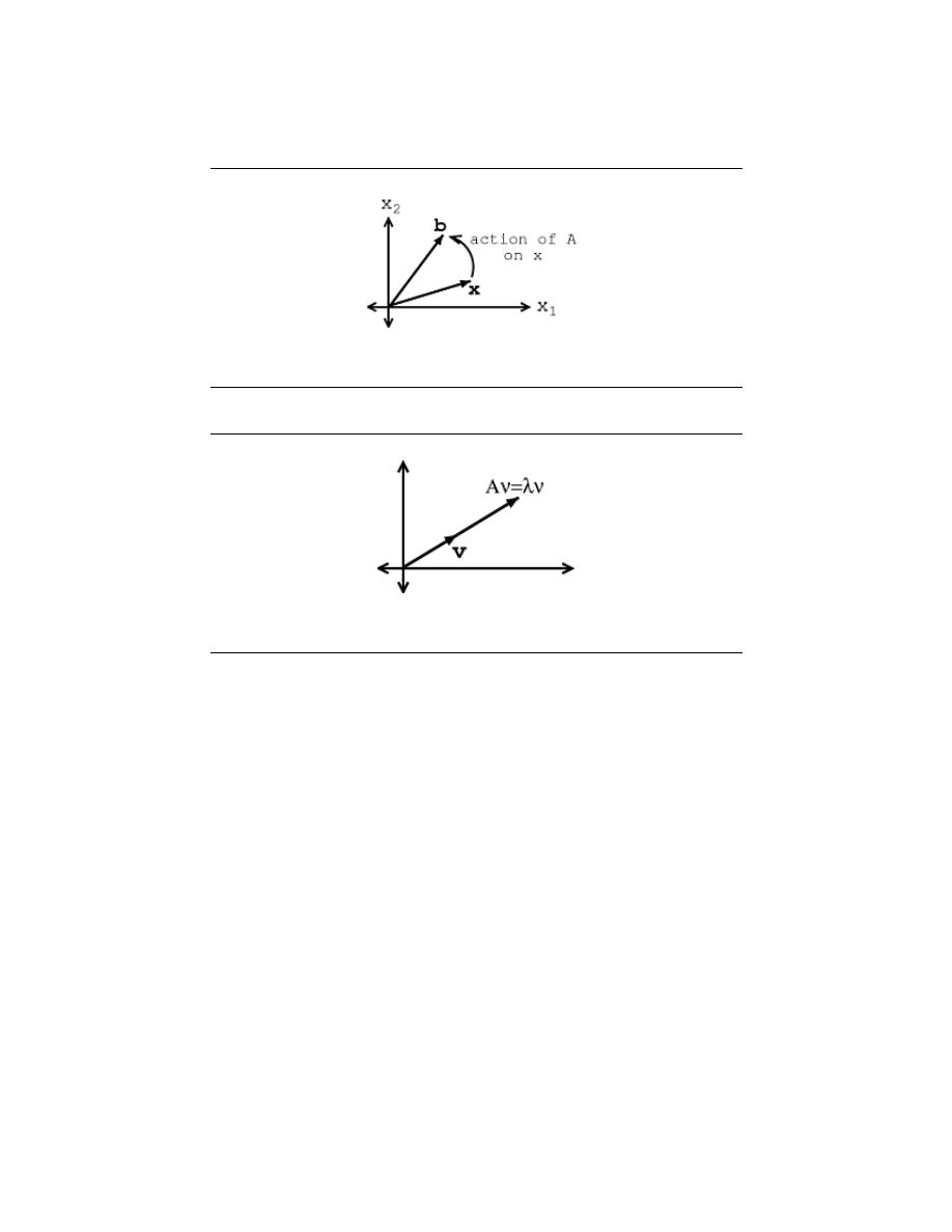
71
Figure 4.6:
Represents Equation 4.1, Ax = b.
Figure 4.7:
Represents Equation 4.2, Av = λv.
4.3.1.1 Graphical Model
Through the two figures below, let us look at the difference between Equation 4.1 and
Equation 4.2.
If v is an eigenvector of A, then only its length changes. See the following figure and
notice how our vector’s length is simply scaled by our variable, λ, called the eigenvalue :
note:
When dealing with a matrix A, eigenvectors are the simplest possible
vectors to operate on.
4.3.1.2 Examples
Exercise 4.3:
From inspection and understanding of eigenvectors, find the two eigenvectors, v
1
and v
2
, of
A =
3
0
0
−1
Also, what are the corresponding eigenvalues, λ
1
and λ
2
? Do not worry if you are
having problems seeing these values from the information given so far, we will look
at more rigorous ways to find these values soon.
Solution:

72
CHAPTER 4. LINEAR ALGEBRA OVERVIEW
The eigenvectors you found should be:
v
1
=
1
0
v
2
=
0
1
And the corresponding eigenvalues are
λ
1
= 3
λ
2
= −1
Exercise 4.4:
Show that these two vectors,
v
1
=
1
1
v
2
=
1
−1
are eigenvectors of A, where A =
3
−1
−1
3
. Also, find the corresponding
eigenvalues.
Solution:
In order to prove that these two vectors are eigenvectors, we will show that these
statements meet the requirements stated in the definition (Definition 4.4: ).
Av
1
=
3
−1
−1
3
1
1
=
2
2
Av
2
=
3
−1
−1
3
1
−1
=
4
−4
These results show us that A only scales the two vectors (i.e. changes their length)
and thus it proves that Equation 4.2 holds true for the following two eigenvalues
that you were asked to find:
λ
1
= 2
λ
2
= 4
If you need more convincing, then one could also easily graph the vectors and their
corresponding product with A to see that the results are merely scaled versions of
our original vectors, v
1
and v
2
.
4.3.2 Calculating Eigenvalues and Eigenvectors
In the above examples, we relied on your understanding of the defintion and on some basic
observations to find and prove the values of the eigenvectors and eigenvalues. However,
as you can probably tell, finding these values will not always be that easy. Below, we
walk through a rigorous and mathematical approach at calculating the eigenvalues and
eigenvectors of a matrix.

73
4.3.2.1 Finding Eigenvalues
Find λ ∈ C such that v 6= 0, where 0 is the ”zero vector.” We will start with Equation 4.2,
and then work our way down until we find a way to explicitly calculate λ.
Av = λv
Av − λv = 0
(A − λI) v = 0
In the previous step, we used the fact that
λv = λIv
where I is the identity matrix.
I =
1
0
. . .
0
0
1
. . .
0
0
0
@@@
..
.
0
. . .
. . .
1
So, A − λI is just a new matrix.
Example 4.5:
Given the following matrix, A, then we can find our new matrix, A − λI.
A =
a
11
a
12
a
21
a
22
A − λI =
a
11
− λ
a
12
a
21
a
22
− λ
If (A − λI) v = 0 for some v 6= 0, then A − λI is not invertible. This means:
det (A − λI) = 0
This determinant (shown directly above) turns out to be a polynomial expression (of order
n). Look at the examples below to see what this means.
Example 4.6:
Starting with matrix A (shown below), we will find the polynomial expression,
where our eigenvalues will be the dependent variable.
A =
3
−1
−1
3
A − λI =
3 − λ
−1
−1
3 − λ
det (A − λI) = (3 − λ)
2
− (−1)
2
= λ
2
− 6λ + 8
λ = {2, 4}

74
CHAPTER 4. LINEAR ALGEBRA OVERVIEW
Example 4.7:
Starting with matrix A (shown below), we will find the polynomial expression,
where our eigenvalues will be the dependent variable.
A =
a
11
a
12
a
21
a
22
A − λI =
a
11
− λ
a
12
a
21
a
22
− λ
det (A − λI) = λ
2
− (a
11
+ a
22
) λ − a
21
a
12
+ a
11
a
22
If you have not already noticed it, calculating the eigenvalues is equivalent to calculating
the roots of
det (A − λI) = c
n
λ
n
+ c
n−1
λ
n−1
+ · · · + c
1
λ + c
0
= 0
conclusion:
Therefore, by simply using calculus to solve for the roots of our
polynomial we can easily find the eigenvalues of our matrix.
4.3.2.2 Finding Eigenvectors
Given an eigenvalue, λ
i
, the associated eigenvectors are given by
Av = λ
i
v
A
v
1
..
.
v
n
=
λ
1
v
1
..
.
λ
n
v
n
set of n equations with n unknowns. Simply solve the n equations to find the eigenvectors.
4.3.3 Main Point
Say the eigenvectors of A, {v
1
, v
2
, . . . , v
n
}, span (Section 4.1.2) C
n
, meaning {v
1
, v
2
, . . . , v
n
}
are linearly independent (Section 4.1.1) and we can write any x ∈ C
n
as
x = α
1
v
1
+ α
2
v
2
+ · · · + α
n
v
n
(4.3)
where {α
1
, α
2
, . . . , α
n
} ∈ C. All that we are doing is rewriting x in terms of eigenvetors of
A. Then,
Ax = A (α
1
v
1
+ α
2
v
2
+ · · · + α
n
v
n
)
Ax = α
1
Av
1
+ α
2
Av
2
+ · · · + α
n
Av
n
Ax = α
1
λ
1
v
1
+ α
2
λ
2
v
2
+ · · · + α
n
λ
n
v
n
= b
Therefore we can write,
x =
X
i
(α
i
v
i
)
and this leads us to the following depicted system:
where in the above figure we have,
b =
X
i
(α
i
λ
i
v
i
)
Main Point:
By breaking up a vector, x, into a combination of eigenvectors,
the calculation of Ax is broken into ”easy to swallow” pieces.

75
Figure 4.8:
Depiction of system where we break our vector, x, into a sum of its
eigenvetors.
4.3.4 Practice Problem
Exercise 4.5:
For the following matrix, A and vector, x, sovle for their product. Try solving it
using two different methods: directly and using eigenvectors.
A =
3
−1
−1
3
x =
5
3
Solution:
Direct Method (use basic matrix multiplication)
Ax =
3
−1
−1
3
5
3
=
12
4
Eigenvectors (use the eigenvectors and eigenvalues we found earlier for this same
matrix)
v
1
=
1
1
v
2
=
1
−1
λ
1
= 2
λ
2
= 4
As shown in Equation 4.3, we want to represent x as a sum of its scaled eigenvectors.
For this case, we have:
x = 4v
1
+ v
2
x =
5
3
= 4
1
1
+
1
−1
Ax = A (4v
1
+ v
2
) = λ
i
(4v
1
+ v
2
)
Therefore, we have
Ax = 4 × 2
1
1
+ 4
1
−1
=
12
4
Notice that this method using eigenvectors required no matrix multiplication. This
may have seemed more complicated here, but just imagine A being really big, or
even just a few dimensions larger!

76
CHAPTER 4. LINEAR ALGEBRA OVERVIEW
5.4 Matrix Diagonalization
From our understanding of eigenvalues and eigenvectors we have discovered several things
about our operator matrix, A. We know that if the eigenvectors of A span C
n
and we know
how to express any vector x in terms of {v
1
, v
2
, . . . , v
n
}, then we have the operator A all
figured out. If we have A acting on x, then this is equal to A acting on the combinations of
eigenvectors. Which we know proves to be fairly easy!
We are still left with two questions that need to be addressed:
1. - When do the eigenvectors {v
1
, v
2
, . . . , v
n
} of A span C
n
(assuming {v
1
, v
2
, . . . , v
n
}
are linearly independent)?
2. - How do we express a given vector x in terms of {v
1
, v
2
, . . . , v
n
}?
4.4.1 Answer to Question #1
Question #1:
When do the eigenvectors {v
1
, v
2
, . . . , v
n
} of A span C
n
?
If A has n distinct eigenvalues
∀i, i 6= j : λ
i
6= λ
j
where i and j are integers, then A has n linearly independent eigenvectors {v
1
, v
2
, . . . , v
n
}
which then span C
n
.
aside:
The proof of this statement is not very hard, but is not really interesting
enough to include here. If you wish to research this idea further, read Strang, G.,
”Linear Algebra and its Application” for the proof.
Furthermore, n distinct eigenvalues means
det (A − λI) = c
n
λ
n
+ c
n−1
λ
n−1
+ · · · + c
1
λ + c
0
= 0
has n distinct roots.
4.4.2 Answer to Question #2
Question #2:
How do we express a given vector x in terms of {v
1
, v
2
, . . . , v
n
}?
We want to find {α
1
, α
2
, . . . , α
n
} ∈ C such that
x = α
1
v
1
+ α
2
v
2
+ · · · + α
n
v
n
(4.4)
In order to find this set of variables, we will begin by collecting the vectors {v
1
, v
2
, . . . , v
n
}
as columns in a n×n matrix V .
V =
..
.
..
.
..
.
v
1
v
2
. . .
v
n
..
.
..
.
..
.
Now Equation 4.4 becomes
x =
..
.
..
.
..
.
v
1
v
2
. . .
v
n
..
.
..
.
..
.
α
1
..
.
α
n

77
or
x = V α
which gives us an easy form to solve for our variables in question, α:
α = V
−1
x
Note that V is invertible since it has n linearly independent columns.
4.4.2.1 Aside
Let us recall our knowledge of functions and there basis and examine the role of V .
x = V α
x
1
..
.
x
n
= V
α
1
..
.
α
n
where α is just x expressed in a different basis (Section 4.1.3):
x = x
1
1
0
..
.
0
+ x
2
0
1
..
.
0
+ · · · + x
n
0
0
..
.
1
x = α
1
..
.
v
1
..
.
+ α
2
..
.
v
2
..
.
+ · · · + α
n
..
.
v
n
..
.
V transforms x from the standard basis to the basis {v
1
, v
2
, . . . , v
n
}
4.4.3 Matrix Diagonalization and Output
We can also use the vectors {v
1
, v
2
, . . . , v
n
} to represent the output, b, of a system:
b = Ax = A (α
1
v
1
+ α
2
v
2
+ · · · + α
n
v
n
)
Ax = α
1
λ
1
v
1
+ α
2
λ
2
v
2
+ · · · + α
n
λ
n
v
n
= b
Ax =
..
.
..
.
..
.
v
1
v
2
. . .
v
n
..
.
..
.
..
.
λ
1
α
1
..
.
λ
1
α
n
Ax = V Λα
Ax = V ΛV
−1
x
where Λ is the matrix with the eigenvalues down the diagonal:
Λ =
λ
1
0
. . .
0
0
λ
2
. . .
0
..
.
..
.
. .
.
..
.
0
0
. . .
λ
n
Finally, we can cancel out the x and are left with a final equation for A:
A = V ΛV
−1

78
CHAPTER 4. LINEAR ALGEBRA OVERVIEW
Figure 4.9:
Simple illustration of LTI system!
4.4.3.1 Interpretation
For our interpretation, recall our key formulas:
α = V
−1
x
b =
X
i
(α
i
λ
i
v
i
)
We can interpret operating on x with A as:
x
1
..
.
x
n
→
α
1
..
.
α
n
→
λ
1
α
1
..
.
λ
1
α
n
→
b
1
..
.
b
n
where the three steps (arrows) in the above illustration represent the following three oper-
ations:
1. - Transform x using V
−1
, which yields α
2. - Multiplication by Λ
3. - Inverse transform using V , which gives us b
This is the paradigm we will use for LTI systems!
5.5 Eigen-stuff in a Nutshell
4.5.1 A Matrix and its Eigenvector
The reason we are stressing eigenvectors and their importance is because the action of a
matrix A on one of its eigenvectors v is
1. - extremely easy (and fast) to calculate
Av = λv
(4.5)
just multiply v by λ.
2. - easy to interpret: A just scales v, keeping its direction constant and only altering
the vector’s length.
If only every vector were an eigenvector of A....

79
Figure 4.10:
LTI System.
4.5.2 Using Eigenvectors’ Span
Of course, not every vector can be ... BUT ... For certain matrices (including ones with
distinct eigenvalues, λ’s), their eigenvectors span (Section 4.1.2) C
n
, meaning that for any
x ∈ C
n
, we can find {α
1
, α
2
, α
n
} ∈ C such that:
x = α
1
v
1
+ α
2
v
2
+ · · · + α
n
v
n
(4.6)
Given Equation 4.6, we can rewrite Ax = b. This equation is modeled in our LTI system
pictured below:
x =
X
i
(α
i
v
i
)
b =
X
i
(α
i
λ
i
v
i
)
The LTI system above represents our Equation 4.5. Below is an illustration of the steps
taken to go from x to b.
x → α = V
−1
x
→ ΛV
−1
x
→ V ΛV
−1
x = b
where the three steps (arrows) in the above illustration represent the following three oper-
ations:
1. - Transform x using V
−1
- yields α
2. - Action of A in new basis - a multiplication by Λ
3. - Translate back to old basis - inverse transform using a multiplication by V , which
gives us b
5.6 Eigenfunctions of LTI Systems
4.6.1 Introduction
Hopefully you are familiar with the notion of the eigenvectors of a ”matrix system,” if not
they do a quick review of eigen-stuff. We can develop the same ideas for LTI systems acting
on signals. A linear time invariant (LTI) system H operating on a continuous input f (t) to
produce continuous time output y (t)
H [f (t)] = y (t)
(4.7)
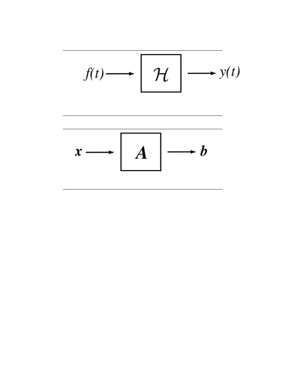
80
CHAPTER 4. LINEAR ALGEBRA OVERVIEW
Figure 4.11:
H [f (t)] = y (t). f and t are continuous time (CT) signals and H is an
LTI operator.
Figure 4.12:
Ax = b where x and b are in C
N
and A is an N x N matrix.
is the mathematically analogous to an N x N matrix A operating on a vector x ∈ C
N
to produce another vector b ∈ C
N
(see Matrices and LTI Systems for an overview).
Ax = b
(4.8)
Just as an eigenvector of A is a v ∈ C
N
such that Av = λv, λ ∈ C,
we can define an eigenfunction (or eigensignal ) of an LTI system H to be a signal
f (t) such that
∀λ, λ ∈ C : H [f (t)] = λf (t)
(4.9)
Eigenfunctions are the simplest possible signals for H to operate on: to calculate the
output, we simply multiply the input by a complex number λ.
4.6.2 Eigenfunctions of any LTI System
The class of LTI systems has a set of eigenfunctions in common: the complex exponentials
e
st
, s ∈ C are eigenfunctions for all LTI systems.
H
e
st
= λ
s
e
st
(4.10)
Note:
While {∀s, s ∈ C : e
st
} are always eigenfunctions of an LTI system, they
are not necessarily the only eigenfunctions.
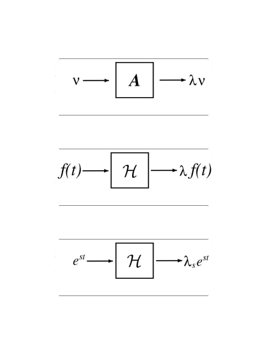
81
Figure 4.13:
Av = λv where v ∈ C
N
is an eigenvector of A.
Figure 4.14:
H [f (t)] = λf (t) where f is an eigenfunction of H.
Figure 4.15:
H
e
st
= λ
s
e
st
where His an LTI system.
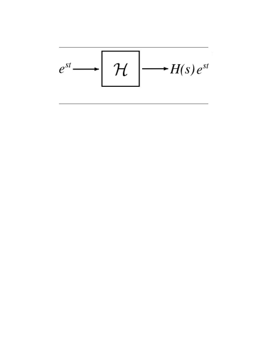
82
CHAPTER 4. LINEAR ALGEBRA OVERVIEW
Figure 4.16:
e
st
is the eigenfunction and H (s) are the eigenvalues.
We can prove Equation 4.10 by expressing the output as a convolution of the input e
st
and the impulse response h (t) of H:
H [e
st
]
=
R
∞
−∞
h (τ ) e
s(t−τ )
dτ
=
R
∞
−∞
h (τ ) e
st
e
−(sτ )
dτ
=
e
st
R
∞
−∞
h (τ ) e
−(sτ )
dτ
(4.11)
Since the expression on the right hand side does not depend on t, it is a constant, λ
s
.
Therefore
H
e
st
= λ
s
e
st
(4.12)
The eigenvalue λ
s
is a complex number that depends on the exponent s and, of course, the
system H. To make these dependencies explicit, we will use the notation H (s) ≡ λ
s
.
Since the action of an LTI operator on its eigenfunctions e
st
is easy to calculate and
interpret, it is convenient to represent an arbitrary signal f (t) as a linear combination of
complex exponentials. The Fourier series gives us this representation for periodic continuous
time signals, while the (slightly more complicated) Fourier transform lets us expand arbitrary
continuous time signals.
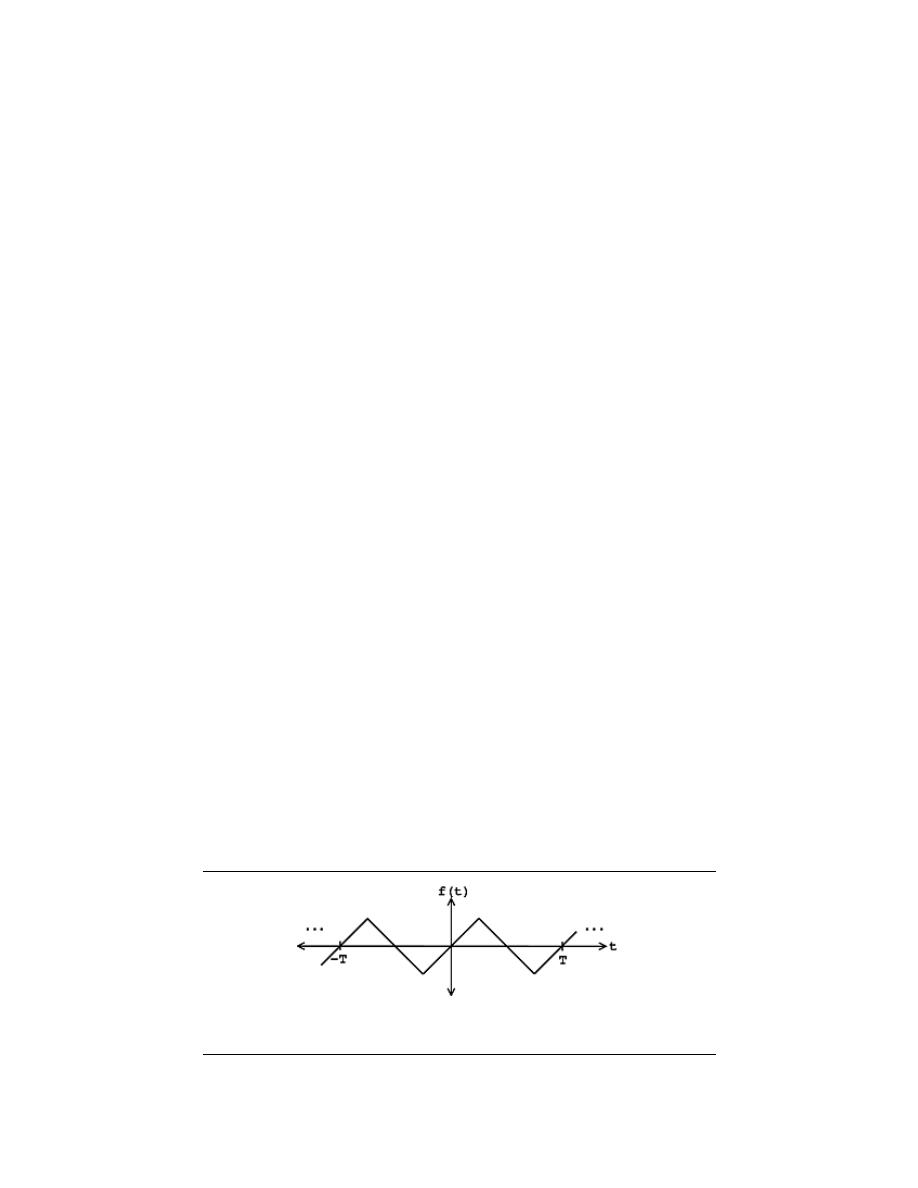
Chapter 5
Fourier Series
6.1 Periodic Signals
Recall that a periodic function is a function that repeats itself exactly after some given
period, or cycle. We represent the defintion of a periodic function mathematically as:
f (t) = f (t + T )
(5.1)
where T > 0 represents the period . Because of this, you may also see a signal referred to
as a T-periodic signal. Any function that satisfies this equation is periodic.
We can think of periodic functions (with period T ) two different ways:
#1) as functions on all of R
#2) or, we can cut out all of the redundancy, and think of them as functions on an
interval [0, T ] (or, more generally, [a, a + T ]). If we know the signal is T-periodic then all
the information of the signal is captured by the above interval.
6.2 Fourier Series: Eigenfunction Approach
5.2.1 Introduction
Since complex exponentials are eigenfunctions of linear time-invariant (LTI) systems, calcu-
lating the output of an LTI system H given e
st
as an input amounts to simple multiplcation,
where H (s) ∈ C is a constant (that depends on s). In the figure below we have a simple
Figure 5.1:
Function over all of R where f (t
0
) = f (t
0
+ T )
83
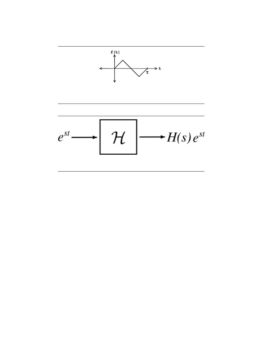
84
CHAPTER 5. FOURIER SERIES
Figure 5.2:
Remove the redundancy of the perioid function so that f (t) is undefined
outside [0, T ].
Figure 5.3:
Simple LTI system.
exponential input that yields the following output:
y (t) = H (s) e
st
(5.2)
Using this and the fact that H is linear, calculating y (t) for combinations of complex
exponentials is also straightforward. This linearity property is depicted in the two equations
below - showing the input to the linear system H on the left side and the output, y (t), on
the right:
1. -
c
1
e
s
1
t
+ c
2
e
s
2
t
→ c
1
H (s
1
) e
s
1
t
+ c
2
H (s
2
) e
s
2
t
2. -
X
n
c
n
e
s
n
t
→
X
n
c
n
H (s
n
) e
s
n
t
The action of H on an input such as those in the two equations above is easy to ex-
plain:
H independently scales each exponential component e
s
n
t
by a different complex
number H (s
n
) ∈ C. As such, if we can write a function f (t) as a combination of complex
exponentials it allows us to:
• - easily calculate the output of H given f (t) as an input (provided we know the
eigenvalues H (s))
• - interpret how H manipulates f (t)

85
5.2.2 Fourier Series
Joseph Fourier
1
demonstrated that an arbitrary T-periodic function f (t) can be written as
a linear combination of harmonic complex sinusoids
f (t) =
∞
X
n=−∞
c
n
e
jω
0
nt
(5.3)
where ω
0
=
2π
T
is the fundamental frequency. For almost all f (t) of practical interest, there
exists c
n
to make Equation 5.3 true. If f (t) is finite energy ( f (t) ∈ L
2
[0, T ]), then the
equality in Equation 5.3 holds in the sense of energy convergence; if f (t) is continuous,
then Equation 5.3 holds pointwise. Also, if f (t) meets some mild conditions (the Dirichlet
conditions), then Equation 5.3 holds pointwise everywhere except at points of discontinuity.
The c
n
- called the Fourier coefficients - tell us ”how much” of the sinusoid e
jω
0
nt
is in
f (t). Equation 5.3 essentially breaks down f (t) into pieces, each of which is easily processed
by an LTI system (since it is an eigenfunction of every LTI system).
Mathematically,
Equation 5.3 tells us that the set of harmonic complex exponentials
∀n, n ∈ Z : e
jω
0
nt
form a basis for the space of T-periodic continuous time functions. Below are a few examples
that are intended to help you think about a given signal or function, f (t), in terms of its
exponential basis functions.
5.2.2.1 Examples
For each of the given functions below, break it down into its ”simpler” parts and find its
fourier coefficients. Click to see the solution.
Exercise 5.1:
f (t) = cos (ω
0
t)
Solution:
The tricky part of the problem is finding a way to represent the above function in
terms of its basis, e
jω
0
nt
. To do this, we will use our knowledge of Euler’s Relation
(Section 2.6.2) to represent our cosine function in terms of the exponential.
f (t) =
1
2
e
jω
0
t
+ e
−(jω
0
t)
Now from this form of our function and from Equation 5.3, by inspection we can
see that our fourier coefficients will be:
c
n
=
1
2
if |n| = 1
0 otherwise
Exercise 5.2:
f (t) = sin (2ω
0
t)
1
http://www-groups.dcs.st-and.ac.uk/∼history/Mathematicians/Fourier.html

86
CHAPTER 5. FOURIER SERIES
Solution:
As done in the previous example, we will again use Euler’s Relation (Section 2.6.2)
to represent our sine function in terms of exponential functions.
f (t) =
1
2j
e
jω
0
t
− e
−(jω
0
t)
And so our fourier coefficients are
c
n
=
−j
2
if n = −1
j
2
if n = 1
0 otherwise
Exercise 5.3:
f (t) = 3 + 4cos (ω
0
t) + 2cos (2ω
0
t)
Solution:
Once again we will use the same technique as was used in the previous two prob-
lems. The break down of our function yields
f (t) = 3 + 4
1
2
e
jω
0
t
+ e
−(jω
0
t)
+ 2
1
2
e
j2ω
0
t
+ e
−(j2ω
0
t)
And from this we can find our fourier coefficients to be:
c
n
=
3 if n = 0
2 if |n| = 1
1 if |n| = 2
0 otherwise
5.2.3 Fourier Coefficients
In general f (t), the Fourier coefficients can be calculated from Equation 5.3 by solving
for c
n
, which requires a little algebraic manipulation (for the complete derivation see the
Fourier coefficients derivation). The end results will yield the following general equation for
the fourier coefficients:
c
n
=
1
T
Z
T
0
f (t) e
−(jω
0
nt)
dt
(5.4)
The sequence of complex numbers {∀n, n ∈ Z : c
n
} is just an alternate representation of the
function f (t). Knowing the Fourier coefficients c
n
is the same as knowing f (t) explicitly
and vice versa.
Given a periodic function, we can transform it into it Fourier series
representation using Equation 5.4. Likewise, we can inverse transform a given sequence
of complex numbers, c
n
, using Equation 5.3 to reconstruct the function f (t).
Along with being a natural representation for signals being manipulated by LTI systems,
the Fourier series provides a description of periodic signals that is convenient in many ways.
By looking at the Fourier series of a signal f (t), we can infer mathematical properties of f (t)
such as smoothness, existence of certain symmetries, as well as the physically meaningful
frequency content.

87
5.2.3.1 Example: Using Fourier Coefficient Equation
Here we will look at a rather simple example that almost requires the use of Equation 5.4
to solve for the fourier coefficients. Once you understand the formula, the solution becomes
a straightforward calculus problem. Find the fourier coefficients for the following equation:
Exercise 5.4:
f (t) =
1 if |t| ≤ T
0 otherwise
Solution:
We will begin by plugging our above function, f (t), into Equation 5.4. Our interval
of integration will now change to match the interval specified by the function.
c
n
=
1
T
Z
T
1
−T
1
(1) e
−(jω
0
nt)
dt
Notice that we must consider two cases: n = 0 and n 6= 0. For n = 0 we can tell
by inspection that we will get
∀n, n = 0 : c
n
=
2T
1
T
For n 6= 0, we will need to take a few more steps to solve. We can begin by looking
at the basic integral of the exponential we have. Remembering our calculus, we
are ready to integrate:
c
n
=
1
T
1
jω
0
n
e
−(jω
0
nt)
|
T
1
t=−T
1
Let us now evaluate the exponential functions for the given limits and expand our
equation to:
c
n
=
1
T
1
− (jω
0
n)
e
−(jω
0
nT
1
)
− e
jω
0
nT
1
Now if we multiple the right side of our equation by
2j
2j
and distribute our negative
sign into the parenthesis, we can utilize Euler’s Relation (Section 2.6.2) to greatly
simplify our expression into:
c
n
=
1
T
2j
jω
0
n
sin (ω
0
nT
1
)
Now, recall earlier that we defined ω
0
=
2π
T
. We can solve this equation for T and
substitute in.
c
n
=
2jω
0
jω
0
n2π
sin (ω
0
nT
1
)
And finally, if we make a few simple cancellations we will arrive at our final answer
for the Fourier coefficients of f (t):
∀n, n 6= 0 : c
n
=
sin (ω
0
nT
1
)
nπ

88
CHAPTER 5. FOURIER SERIES
5.2.4 Summary: Fourier Series Equations
Our first equation (Equation 5.3) is the synthesis equation, which builds our function,
f (t), by combining sinusoids.
Synthesis
f (t) =
∞
X
n=−∞
c
n
e
jω
0
nt
(5.5)
And our second equation (Equation 5.4), termed the analysis equation, reveals how much
of each sinusoid is in f (t).
Analysis
c
n
=
1
T
Z
T
0
f (t) e
−(jω
0
nt)
dt
(5.6)
where we have stated that ω
0
=
2π
T
.
note:
Understand that our interval of integration does not have to be [0, T ] in
our Analysis Equation. We could use any interval [a, a + T ] of length T .
6.3 Derivation of Fourier Coefficients Equation
5.3.1 Introduction
You should already be familiar with the existence of the general Fourier Series equation
(Section 5.2.2), which is written as:
f (t) =
∞
X
n=−∞
c
n
e
jω
0
nt
(5.7)
What we are interested in here is how to determine the Fourier coefficients, c
n
, given a
function f (t). Below we will walk through the steps of deriving the general equation for the
Fourier coefficients of a given function.
5.3.2 Derivation
To solve Equation 5.7 for c
n
, we have to do a little algebraic manipulation. First of all we
will multiply both sides of Equation 5.7 by e
−(jω
0
kt)
, where k ∈ Z.
f (t) e
−(jω
0
kt)
=
∞
X
n=−∞
c
n
e
jω
0
nt
e
−(jω
0
kt)
(5.8)
Now integrate both sides over a given period, T :
Z
T
0
f (t) e
−(jω
0
kt)
dt =
Z
T
0
∞
X
n=−∞
c
n
e
jω
0
nt
e
−(jω
0
kt)
dt
(5.9)
On the right-hand side we can switch the summation and integral along with pulling out
the constant out of the integral.
Z
T
0
f (t) e
−(jω
0
kt)
dt =
∞
X
n=−∞
c
n
Z
T
0
e
jω
0
(n−k)t
dt
!
(5.10)

89
Now that we have made this seemingly more complicated, let us focus on just the integral,
R
T
0
e
jω
0
(n−k)t
dt, on the right-hand side of the above equation. For this intergral we will need
to consider two cases: n = k and n 6= k. For n = k we will have:
∀n, n = k :
Z
T
0
e
jω
0
(n−k)t
dt = T
(5.11)
For n 6= k, we will have:
∀n, n 6= k :
Z
T
0
e
jω
0
(n−k)t
dt =
Z
T
0
cos (jω
0
(n − k) t) dt + j
Z
T
0
sin (jω
0
(n − k) t) dt (5.12)
But cos (jω
0
(n − k) t) has an integer number of periods, n − k, between 0 and T . Imagine
a graph of the cosine; because it has an integer number of periods, there are equal areas
above and below the x-axis of the graph. This statemnt holds true for sin (jω
0
(n − k) t) as
well. What this means is
Z
T
0
cos (jω
0
(n − k) t) dt = 0
(5.13)
as well as the integral involving the sine function. Therefore, we conclude the following
about our intregral of interest:
Z
T
0
e
jω
0
(n−k)t
dt =
T if n = k
0 otherwise
(5.14)
Now let us return our attention to our complicated equation, Equation 5.10, to see if we
can finish finding an equation for our Fourier coefficients. Using the facts that we have just
proven above, we can see that the only time Equation 5.10 will have a nonzero result is
when k and n are equal:
∀n, n = k :
Z
T
0
f (t) e
−(jω
0
nt)
dt = T c
n
(5.15)
Finally, we have our general equation for the Fourier coefficients:
c
n
=
1
T
Z
T
0
f (t) e
−(jω
0
nt)
dt
(5.16)
5.3.2.1 Finding Fourier Coefficients Steps
To find the Fourier coefficients of periodic f (t):
1. - For a given k, multiply f (t) by e
−(jω
0
kt)
, and take the area under the curve (dividing
by T ).
2. - Repeat step (1) forall k ∈ Z.
6.4 Fourier Series in a Nutshell
5.4.1 Introduction
The convolution integral is the fundamental expression relating the input and output of an
LTI system. However, it has three shortcomings:
1. - It can be tedious to calculate.
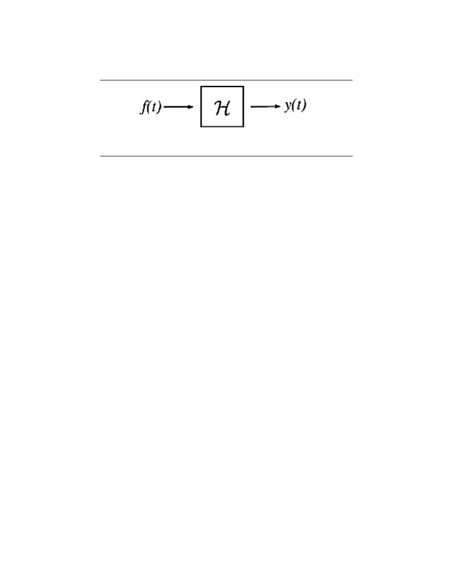
90
CHAPTER 5. FOURIER SERIES
Figure 5.4:
Transfer Functions modeled as LTI System.
2. - It offers only limited physical interpretation of what the system is actually doing.
3. - It gives little insight on how to design systems to accomplish certain tasks.
The Fourier Series, along with the Fourier Transform and Laplace Transofrm, provides a
way to address these three points. Central to all of these methods is the concept of an
eigenfunction (or eigenvector). We will look at how we can rewrite any given signal, f (t),
in terms of complex exponentials.
In fact, by making our notions of signals and linear systems more mathematically ab-
stract, we will be able to draw enlightening parallels between signals and systems and linear
algebra.
5.4.2 Eigenfunctions and LTI Systems
The action of a LTI system H [. . . ] on one of its eigenfunctions e
st
is
1. - extremely easy (and fast) to calculate
H [st] = H [s] e
st
(5.17)
2. - easy to interpret: H [. . . ] just scales e
st
, keeping its frequency constant.
If only every function were an eigenfunction of H [. . . ] ...
5.4.2.1 LTI System
... of course, not every function can be, but for LTI systems, their eigenfunctions span
(Section 4.1.2) the space of periodic functions, meaning that for (almost) any periodic
function f (t) we can find {c
n
} where n ∈ Z and c
i
∈ C such that:
f (t) =
∞
X
n=−∞
c
n
e
jω
0
nt
(5.18)
Given Equation 5.18, we can rewrite H [t] = y (t) as the following system
where we have:
f (t) =
X
n
c
n
e
jω
0
nt
y (t) =
X
n
c
n
H (jω
0
n) e
jω
0
nt
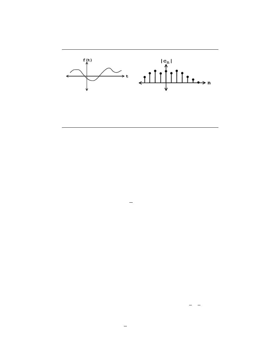
91
(a)
(b)
Figure 5.5:
We begin with our smooth signal f (t) on the left, and then use the Fourier
series to find our Fourier coefficients - shown in the figure on the right.
This transformation from f (t) to y (t) can also be illustrated through the process below.
Note that each arrow indicates an operation on our signal or coefficients.
f (t) → {c
n
} → {c
n
H (jω
0
n)} → y (t)
(5.19)
where the three steps (arrows) in the above illustration represent the following three oper-
ations:
1. - Transform with analysis (Fourier Coefficient equation):
c
n
=
1
T
Z
T
0
f (t) e
−(jω
0
nt)
dt
2. - Action of H on the Fourier series - equals a multiplication by H (jω
0
n)
3. - Translate back to old basis - inverse transform using our synthesis equation from the
Fourier series:
y (t) =
∞
X
n=−∞
c
n
e
jω
0
nt
5.4.3 Physical Interpretation of Fourier Series
The Fourier series {c
n
} of a signal f (t), defined in Equation 5.18, also has a very important
physical interpretation. Coefficient c
n
tells us ”how much” of frequency ω
0
n is in the signal.
Signals that vary slowly over time - smooth signals - have large c
n
for small n.
Signals that vary quickly with time - edgy or noisy signals - will have large c
n
for large
n.
Example 5.1:
Periodic Pulse
We have the following pulse function, f (t), over the interval
−
T
2
,
T
2
:
Using our formula for the Fourier coefficients,
c
n
=
1
T
Z
T
0
f (t) e
−(jω
0
nt)
dt
(5.20)
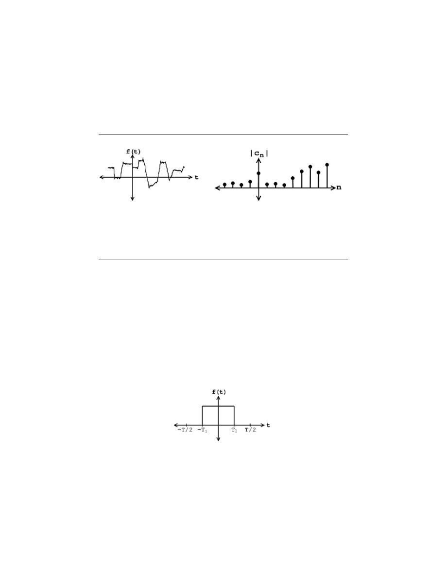
92
CHAPTER 5. FOURIER SERIES
(a)
(b)
Figure 5.6:
We begin with our noisy signal f (t) on the left, and then use the Fourier
series to find our Fourier coefficients - shown in the figure on the right.
Figure 5.7:
Periodic Signal f (t)

93
Figure 5.8:
Our Fourier coefficients when T
1
=
T
8
we can easily calculate our c
n
. We will leave the calculation as an exercise for you!
After solving the the equation for our f (t), you will get the following results:
c
n
=
2T
1
T
if n = 0
2sin(ω
0
nT
1
)
nπ
if n 6= 0
(5.21)
For T
1
=
T
8
, see the figure below for our results:
Our signal f (t) is flat except for two edges (discontinuities). Because of this, c
n
around n = 0 are large and c
n
gets smaller as n approaches infinity.
question:
Why does c
n
= 0 for n = {. . . , −4, 4, 8, 16, . . . }? (What part
of e
−(jω
0
nt)
lies over the pulse for these values of n?)
6.5 Fourier Series Properties
We will begin by refreshing your memory of our basic Fourier series equations:
f (t) =
∞
X
n=−∞
c
n
e
jω
0
nt
(5.22)
c
n
=
1
T
Z
T
0
f (t) e
−(jω
0
nt)
dt
(5.23)
Let F · denote the tranformation from f (t) to the Fourier coefficients
F f (t) = ∀n, n ∈ Z
F · maps complex valued functions to sequences of complex numbers.
5.5.1 Linearity
F · is a linear transformation .
Theorem 5.1:
If F f (t) = c
n
and F g (t) = d
n
. Then
∀α, α ∈ C : Fαf (t) = αc
n
and
F f (t) + g (t) = c
n
+ d
n

94
CHAPTER 5. FOURIER SERIES
Proof:
Easy. Just linearety of integral.
F f (t) + g (t)
=
∀n, n ∈ Z :
R
T
0
(f (t) + g (t)) e
−(jω
0
nt)
dt
=
∀n, n ∈ Z :
1
T
R
T
0
f (t) e
−(jω
0
nt)
dt +
1
T
R
T
0
g (t) e
−(jω
0
nt)
dt
=
∀n, n ∈ Z : c
n
+ d
n
=
c
n
+ d
n
(5.24)
5.5.2 Shifting
Shifting in time equals a phase shift of Fourier coefficients
Theorem 5.2:
F f (t − t
0
) = e
−(jω
0
nt
0
)
c
n
if c
n
= |c
n
|e
j∠c
n
, then
|e
−(jω
0
nt
0
)
c
n
| = |e
−(jω
0
nt
0
)
||c
n
| = |c
n
|
∠e
−(jω
0
t
0
n)
= ∠c
n
− ω
0
t
0
n
Proof:
F f (t − t
0
)
=
∀n, n ∈ Z :
1
T
R
T
0
f (t − t
0
) e
−(jω
0
nt)
dt
=
∀n, n ∈ Z :
1
T
R
T −t
0
−t
0
f (t − t
0
) e
−(jω
0
n(t−t
0
))
e
−(jω
0
nt
0
)
dt
=
∀n, n ∈ Z :
1
T
R
T −t
0
−t
0
f ˜
t
e
−
(
jω
0
n˜
t
)e
−(jω
0
nt
0
)
dt
=
∀n, n ∈ Z : e
−
(
jω
0
n˜
t
)c
n
(5.25)
5.5.3 Parseval’s Relation
Z
T
0
(|f (t) |)
2
dt = T
∞
X
n=−∞
(|c
n
|)
2
(5.26)
Parseval’s relation allows us to calculate the energy of a signal from its Fourier series.
note:
Parseval tells us that the Fourier series maps L
2
([0, T ]) to l
2
(Z).
Exercise 5.5:
For f (t) to have ”finite energy,” what do the c
n
do as n → ∞?
Solution:
(|c
n
|)
2
< ∞ for f (t) to have finite energy.
Exercise 5.6:
If ∀n, |n| > 0 : c
n
=
1
n
, is f ∈ L
2
([0, T ])?
Solution:
Yes, because (|c
n
|)
2
=
1
n
2
, which is summable.
Exercise 5.7:
Now, if ∀n, |n| > 0 : c
n
=
1
√
n
, is f ∈ L
2
([0, T ])?
Solution:
No, because (|c
n
|)
2
=
1
n
, which is not summable.
The rate of decay of the Fourier series determines if f (t) has finite energy.
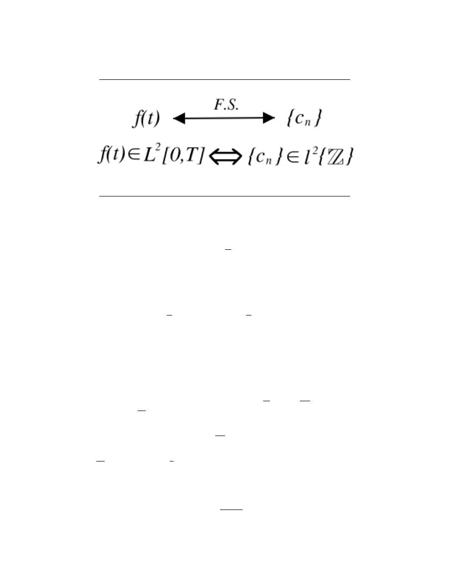
95
Figure 5.9
5.5.4 Differentiation in Fourier Domain
F f (t) = c
n
⇒ F
d
dt
f (t) = jnω
0
c
n
(5.27)
Since
f (t) =
∞
X
n=−∞
c
n
e
jω
0
nt
(5.28)
then
d
dt
f (t)
=
P
∞
n=−∞
c
n
d
dt
e
jω
0
nt
=
P
∞
n=−∞
c
n
jω
0
ne
jω
0
nt
(5.29)
A differentiator attenuates the low frequencies in f (t) and accentuates the high frequencies.
It removes general trends and accentuates areas of sharp variation.
note:
A common way to mathematically measure the smoothness of a function
f (t) is to see how many derivatives are finite energy.
This is done by looking at the Fourier coefficients of the signal, specifically how fast they
decay as n → ∞. If F f (t) = c
n
and |c
n
| has the form
1
n
k
, then F
d
m
dt
m
f (t) = (jnω
0
)
m
c
n
and has the form
n
m
n
k
. So for the m
th
derivative to have finite energy, we need
X
|
n
m
n
k
|
2
!
< ∞
thus
n
m
n
k
decays faster than
1
n
which implies that
2k − 2m > 1
or
k >
2m + 1
2
Thus the decay rate of the Fourier series dictates smoothness.

96
CHAPTER 5. FOURIER SERIES
5.5.5 Integration in the Fourier Domain
If
F f (t) = c
n
(5.30)
then
F
Z
t
−∞
f (τ ) dτ =
1
jω
0
n
c
n
(5.31)
note:
If c
0
6= 0, this expression doesn’t make sense.
Integration accentuates low frequencies and attenuates high frequencies. Integrators
bring out the general trends in signals and supress short term variation (which is noise in
many cases). Integrators are much nicer than differentiators.
5.5.6 Signal Multiplication
Given a signal f (t) with Fourier coefficients c
n
and a signal g (t) with Fourier coefficients
d
n
, we can define a new signal, y (t), where y (t) = f (t) g (t). We find that the Fourier
Series representation of y (t), e
n
, is such that e
n
=
P
∞
k=−∞
(c
k
d
n−k
). This is to say that
signal multiplication in the time domain is equivalent to discrete-time convolution in the
frequency domain. The proof of this is as follows
e
n
=
1
T
R
T
0
f (t) g (t) e
−(jω
0
nt)
dt
=
1
T
R
T
0
P
∞
k=−∞
c
k
e
jω
0
kt
g (t) e
−(jω
0
nt)
dt
=
P
∞
k=−∞
c
k
1
T
R
T
0
g (t) e
−(jω
0
(n−k)t)
dt
=
P
∞
k=−∞
(c
k
d
n−k
)
(5.32)
6.6 Symmetry Properties of the Fourier Series
5.6.1 Symmetry Properties
5.6.1.1 Real Signals
Real signals have a conjugate symmetric Fourier series.
Theorem 5.3:
If f (t) is real it implies that f (t) = f (t)
∗
(f (t)
∗
is the complex conjugate of
f (t)), then c
n
= c
−n
∗
which implies that Re (c
n
) = Re (c
−n
), i.e. the real part of
c
n
is even, and Im (c
n
) = − (Im (c
−n
)), i.e. the imaginary part of c
n
is odd. See
Figure 5.10. It also implies that |c
n
| = |c
−n
|, i.e. that magnitude is even, and that
∠c
n
= (∠ − c
−n
), i.e. the phase is odd.
Proof:
c
−n
=
1
T
R
T
0
f (t) e
jω
0
nt
dt
=
∀t, f (t) = f (t)
∗
:
1
T
R
T
0
f (t)
∗
e
−(jω
0
nt)
dt
∗
=
1
T
R
T
0
f (t) e
−(jω
0
nt)
dt
∗
=
c
n
∗
(5.33)
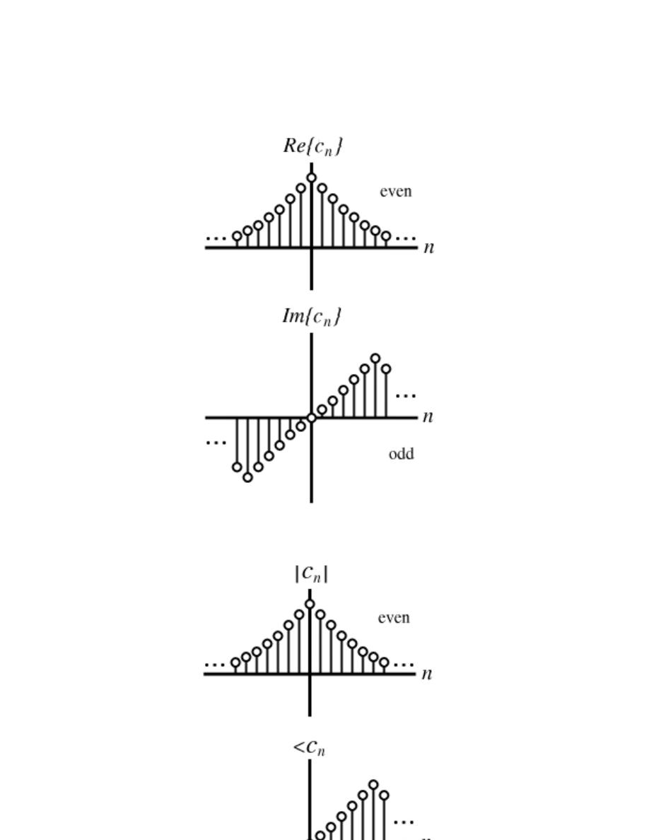
97
(a)
(b)
Figure 5.10:
(a) Re (c
n
) = Re (c
−n
), and Im (c
n
) = − (Im (c
−n
)). (b) |c
n
| = |c
−n
|, and
∠c
n
= (∠ − c
−n
).

98
CHAPTER 5. FOURIER SERIES
5.6.1.2 Real and Even Signals
Real and even signals have real and even Fourier series.
Theorem 5.4:
If f (t) = f (t)
∗
and f (t) = (f (−t)), i.e. the signal is real and even, then c
n
= c
−n
and c
n
= c
n
∗
.
Proof:
c
n
=
1
T
R
T
2
−
(
T
2
)
f (t) e
−(jω
0
nt)
dt
=
1
T
R
0
−
(
T
2
) f (t) e
−(jω
0
nt)
dt +
1
T
R
T
2
0
f (t) e
−(jω
0
nt)
dt
=
1
T
R
T
2
0
f (−t) e
jω
0
nt
dt +
1
T
R
T
2
0
f (t) e
−(jω
0
nt)
dt
=
2
T
R
T
2
0
f (t) cos (ω
0
nt) dt
(5.34)
f (t) and cos (ω
0
nt) are both real which implies that c
n
is real. Also cos (ω
0
nt) =
cos (− (ω
0
nt)) so c
n
= c
−n
. It is also easy to show that f (t) = 2
P
∞
n=0
(c
n
cos (ω
0
nt))
since f (t), c
n
, and cos (ω
0
nt) are all real and even.
5.6.1.3 Real and Odd Signals
Real and odd signals have Fourier Series that are odd and purely imaginary.
Theorem 5.5:
If f (t) = − (f (−t)) and f (t) = f (t)
∗
, i.e.
the signal is real and odd, then
c
n
= −c
−n
and c
n
= − (c
n
∗
), i.e. c
n
is odd and purely imaginary.
Proof:
Do it at home.
If f (t) is odd, then we can expand it in terms of sin (ω
0
nt):
f (t) =
∞
X
n=1
(2c
n
sin (ω
0
nt))
5.6.2 Summary
In summary, we can find f
e
(t), an even function, and f
o
(t), an odd function, such that
f (t) = f
e
(t) + f
o
(t)
(5.35)
which implies that, for any f (t), we can find {a
n
} and {b
n
} such that
f (t) =
∞
X
n=0
(a
n
cos (ω
0
nt)) +
∞
X
n=1
(b
n
sin (ω
0
nt))
(5.36)
Example 5.2:
Triangle Wave
f (t) is real and odd.
c
n
=
4A
jπ
2
n
2
if n = {. . . , −11, −7, −3, 1, 5, 9, . . . }
−
4A
jπ
2
n
2
if n = {. . . , −9, −5, −1, 3, 7, 11, . . . }
0 if n = {. . . , −4, −2, 0, 2, 4, . . . }
Does c
n
= −c
−n
?
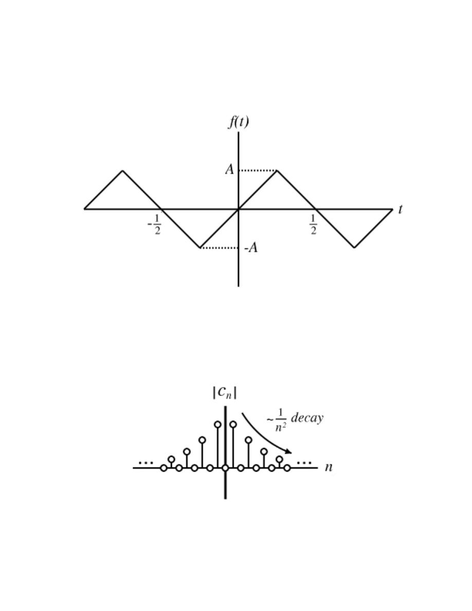
99
Figure 5.11:
T = 1 and ω
0
= 2π.
Figure 5.12:
The Fourier series of a triangle wave.

100
CHAPTER 5. FOURIER SERIES
Note:
We can often gather information about the smoothness of a signal by
examining its Fourier coefficients.
Take a look at the above examples. The pulse and sawtooth waves are not continuous and
there Fourier series’ fall off like
1
n
. The triangle wave is continuous, but not differentiable
and its Fourier series falls off like
1
n
2
.
The next 3 properties will give a better feel for this.
6.7 Circular Convolution Property of Fourier Series
5.7.1 Signal Circular Convolution
Given a signal f (t) with Fourier coefficients c
n
and a signal g (t) with Fourier coefficients
d
n
, we can define a new signal, v (t), where v (t) = (f (t) @@g (t)) We find that the Fourier
Series representation of y (t), a
n
, is such that a
n
= c
n
d
n
. (f (t) @@g (t)) is the circular
convolution of two periodic signals and is equivilent to the convolution over one interval,
i.e. (f (t) @@g (t)) =
R
T
0
R
T
0
f (τ ) g (t − τ ) dτ dt.
note:
Circular convolution in the time domain is equivalent to multiplication of
the Fourier coefficients.
This is proved as follows
a
n
=
1
T
R
T
0
v (t) e
−(jω
0
nt)
dt
=
1
T
2
R
T
0
R
T
0
f (τ ) g (t − τ ) dτ e
−(jω
0
nt)
dt
=
1
T
R
T
0
f (τ )
1
T
R
T
0
g (t − τ ) e
−(jω
0
nt)
dt
dτ
=
∀ν, ν = t − τ :
1
T
R
T
0
f (τ )
1
T
R
T −τ
−τ
g (ν) e
−(jω
0
(ν+τ ))
dν
dτ
=
1
T
R
T
0
f (τ )
1
T
R
T −τ
−τ
g (ν) e
−(jω
0
nν)
dν
e
−(jω
0
nτ )
dτ
=
1
T
R
T
0
f (τ ) d
n
e
−(jω
0
nτ )
dτ
=
d
n
1
T
R
T
0
f (τ ) e
−(jω
0
nτ )
dτ
=
c
n
d
n
(5.37)
Example 5.3:
Take a look at a square pulse with a period, T
1
=
T
4
:
For this signal
c
n
=
(
1
T
if n = 0
1
2
sin
(
π
2
n
)
π
2
n
otherwise
Exercise 5.8:
What signal has Fourier coefficients a
n
= c
n
2
=
1
4
sin
2
(
π
2
n
)
(
π
2
n
)
2
?
Solution:
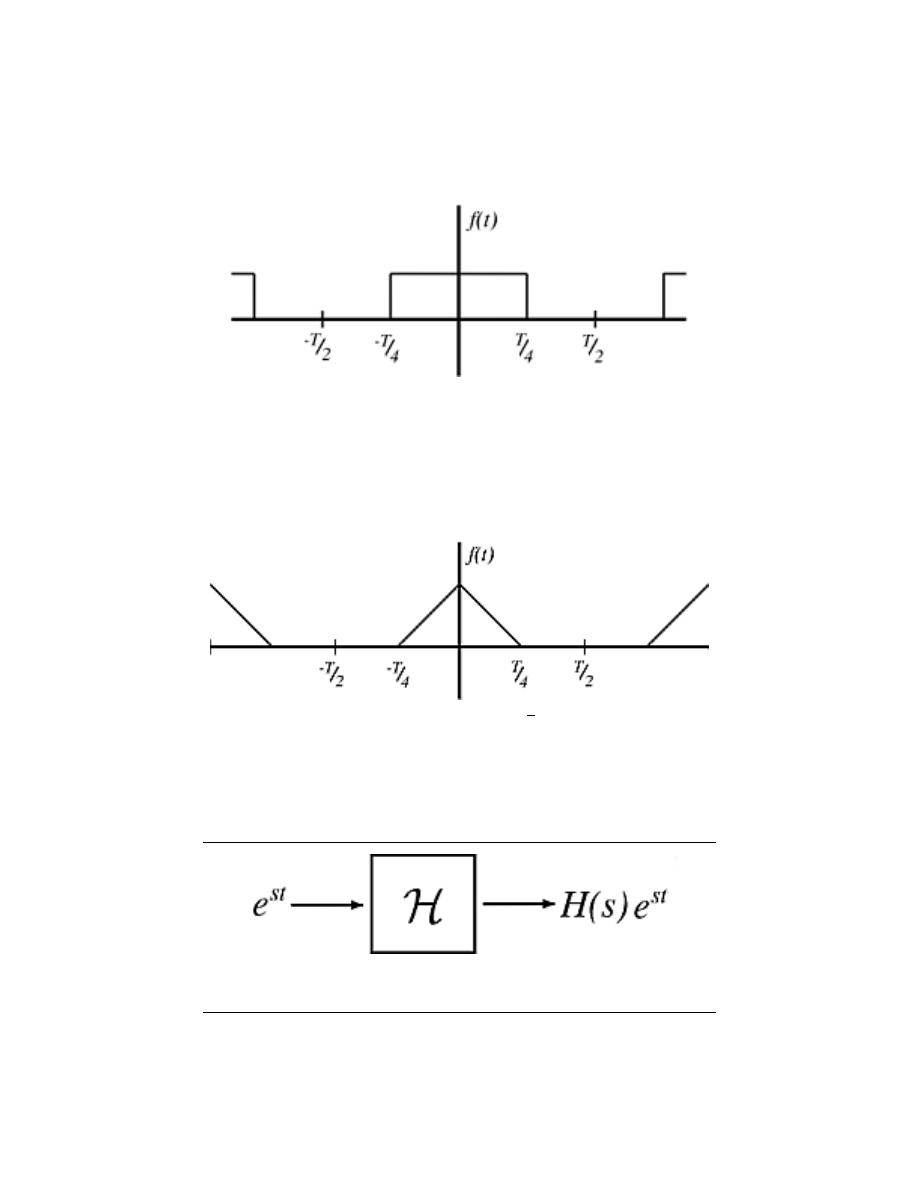
101
Figure 5.13
Figure 5.14:
A triangle pulse train with a period of
T
4
.
Figure 5.15:
Input and output signals to our LTI system.
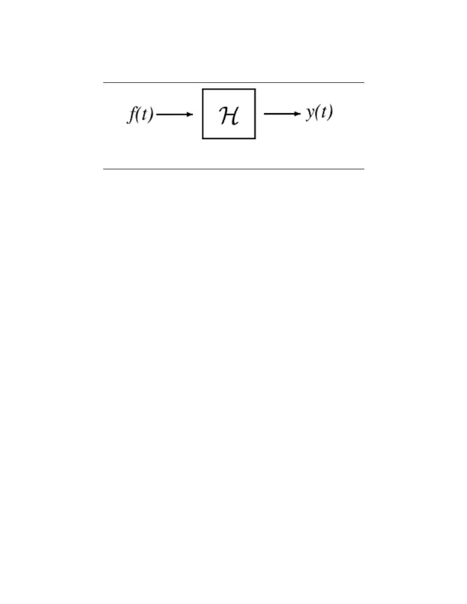
102
CHAPTER 5. FOURIER SERIES
Figure 5.16:
LTI system
6.8 Fourier Series and LTI Systems
5.8.1 Introducing the Fourier Series to LTI Systems
Before looking at this module, one should be familiar with the concepts of eigenfunction
and LTI systems. Recall, for H LTI system we get the following relationship
where e
st
is an eigenfunction of H. Its corresponding eigenvalue H (s) can be calculated
using the impluse response h (t)
H (s) =
Z
∞
−∞
h (τ ) e
−(sτ )
dτ
So, using the Fourier Series expansion for periodic f (t) where we input
f (t) =
X
n
c
n
e
jω
0
nt
into the system
our output y (t) will be
y (t) =
X
n
H (jω
0
n) c
n
e
jω
0
nt
So we can see that by applying the fourier series expansion equations, we can go from f (t)
to c
n
and vice versa, and we do the same for our output, y (t)
5.8.2 Effects of Fourier Series
We can think of an LTI system as shaping the frequency content of the input. Keep in
mind the basic LTI system we presented above in Figure 5.16. The LTI system, H, simply
multiplies all of our Fourier coefficients and scales them.
Given the Fourier coefficients {c
n
} of the input and the eigenvalues of the system
{H (jw
0
n)}, the Fouriers series of the output is {H (jw
0
n) c
n
} (simple term-by-term multi-
plication).
note:
The eigenvalues H (jw
0
n) completely describe what a LTI system does to
periodic signals with period T = 2πw
0
Example 5.4:
What does this system do?
Example 5.5:
What about this system?
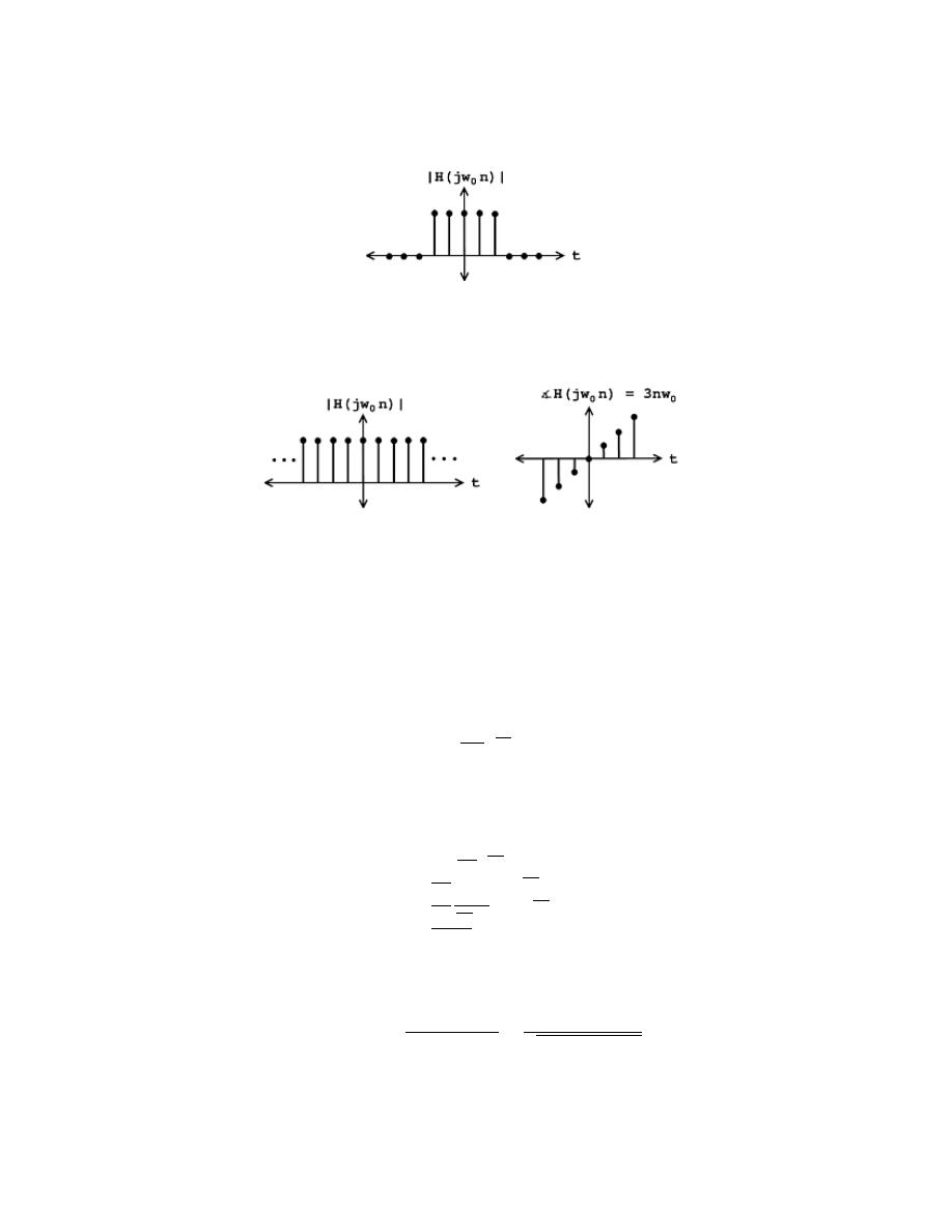
103
Figure 5.17
(a)
(b)
Figure 5.18
5.8.3 Examples
Example 5.6:
RC Circuit
h (t) =
1
RC
e
−t
RC
u (t)
What does this system do to the Fourier Series of an input f (t)?
Calculate the eigenvalues of this system
H (s)
=
R
∞
−∞
h (τ ) e
−(sτ )
dτ
=
R
∞
0
1
RC
e
−τ
RC
e
−(sτ )
dτ
=
1
RC
R
∞
0
e
(−τ )
(
1
RC
+s
)dτ
=
1
RC
1
1
RC
+s
e
(−τ )
(
1
RC
+s
)|
∞
τ =0
=
1
1+RCs
(5.38)
Now, say we feed the RC circuit a periodic (period T = 2πw
0
) input f (t).
Look at the eigenvalues for s = jw
0
n
|H (jw
0
n) | =
1
|1 + RCjw
0
n|
=
1
√
1 + R
2
C
2
w
0
2
n
2
The RC circuit is a lowpass system: it passes low frequencies ( n around 0) and
attenuates high frequencies (large n).

104
CHAPTER 5. FOURIER SERIES
Example 5.7:
Square pulse wave througth RC circuit
•- Input Signal: Taking the fourier series of f (t)
c
n
=
1
2
sin
π
2
n
π
2
n
1
t
at n = 0
•- System: eigenvalues
H (jw
0
n) =
1
1 + jRCw
0
n
•- Output Signal: Taking the fourier series of y (t)
d
n
= H (jw
0
n) c
n
=
1
1 + jRCw
0
n
1
2
sin
π
2
n
π
2
n
d
n
=
1
1 + jRCw
0
n
1
2
sin
π
2
n
π
2
n
y (t) =
X
d
n
e
jw
0
nt
What can we infer about y (t) from {d
n
}?
1.- Is y (t) real?
2.- Is y (t) even symmetric? odd symmetric?
3.- Qualitatively, what does y (t) look like? Is it ”smoother” than f (t)? (decay
rete of d
n
vs. c
n
)
d
n
=
1
1 + jRCw
0
n
1
2
sin
π
2
n
π
2
n
|d
n
| =
1
q
1 + (RCw
0
)
2
n
2
1
2
sin
π
2
n
π
2
n
6.9 Convergence of Fourier Series
5.9.1 Introduction
Before looking at this module, hopefully you have become fully convinced of the fact that
any periodic (pg ??) function, f (t), can be represented as a sum of complex sinusoids.
If you are not, then try looking back at eigen-stuff in a nutshell or eigenfunctions of LTI
systems. We have shown that we can represent a signal as the sum of exponentials through
the Fourier Series equations below:
f (t) =
X
n
c
n
e
jω
0
nt
(5.39)
c
n
=
1
T
Z
T
0
f (t) e
−(jω
0
nt)
dt
(5.40)

105
Joseph Fourier
2
insisted that these equations were true, but could not prove it. Lagrange
publicly ridiculed Fourier, and said that only continuous functions can be represented by
Equation 5.39 (indeed he proved that Equation 5.39 holds for continuous-time functions).
However, we know now that the real truth lies in between Fourier and Lagrange’s positions.
5.9.2 Understanding the Truth
Formulating our question mathematically, let
f
0
N
(t) =
N
X
n=−N
c
n
e
jω
0
nt
where c
n
equals the Fourier coefficients of f (t) (see Equation 5.40).
f
0
N
(t) is a ”partial reconstruction” of f (t) using the first 2N+1 Fourier coefficients.
f
0
N
(t) approximates f (t), with the approximation getting better and better as N gets
large. Therefore, we can think of the set {∀N, N = {0, 1, . . . } : f
0
N
(t)} as a sequence of
functions , each one approximating f (t) better than the one before.
The question is, does this sequence converge to f (t)? Does f
0
N
(t) → f (t) as N → ∞?
We will try to answer this question by thinking about convergence in two different ways:
1. - Looking at the energy of the error signal:
e
N
(t) = f (t) − f
0
N
(t)
2. - Looking at lim
N →∞
f
0
N
(t) at each point and comparing to f (t).
5.9.2.1 Approach #1
Let e
N
(t) be the difference (i.e. error) between the signal f (t) and its partial reconstruction
f
0
N
(t)
e
N
(t) = f (t) − f
0
N
(t)
(5.41)
If f (t) ∈ L
2
([0, T ]) (finite energy), then the energy of e
N
(t) → 0 as N → ∞ is
Z
T
0
(|e
N
(t) |)
2
dt =
Z
T
0
(f (t) − f
0
N
(t))
2
dt → 0
(5.42)
We can prove this equation using Parseval’s relation:
lim
N →∞
Z
T
0
(|f (t) − f
0
N
(t) |)
2
dt = lim
N →∞
∞
X
N =−∞
(|F
n
f (t) − F
n
f
0
N
(t) |)
2
= lim
N →∞
X
|n|>N
(|c
n
|)
2
= 0
where the last equation before zero is the tail sum of the Fourier Series, which approaches
zero because f (t) ∈ L
2
([0, T ]). Since physical systems respond to energy, the Fourier Series
provides an adequate representation for all f (t) ∈ L
2
([0, T ]) equaling finite energy over one
period.
5.9.2.2 Approach #2
The fact that e
N
→ 0 says nothing about f (t) and lim
N →∞
f
0
N
(t) being equal at a given point.
Take the two functions graphed below for example:
2
http://www-groups.dcs.st-and.ac.uk/∼history/Mathematicians/Fourier.html
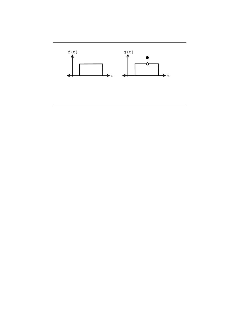
106
CHAPTER 5. FOURIER SERIES
(a)
(b)
Figure 5.19
Given these two functions, f (t) and g (t), then we can see that for all t, f (t) 6= g (t),
but
Z
T
0
(|f (t) − g (t) |)
2
dt = 0
From this we can see the following relationships:
energyconvergence 6= pointwiseconvergence
pointwiseconvergence ⇒ convergenceinL
2
([0, T ])
However, the reverse of the above statement does not hold true.
It turns out that if f (t) has a discontinuity (as can be seen in figure of g (t) above) at
t
0
, then
f (t
0
) 6= lim
N →∞
f
0
N
(t
0
)
But as long as f (t) meets some other fairly mild conditions, then
f (t
0
) = lim
N →∞
f
0
N
(t
0
)
if f (t) is continuous at t = t
0
.
6.10 Dirichlet Conditions
Named after the German mathematician, Peter Dirichlet, the Dirichlet conditions are
the sufficient conditions to guarantee existence and convergence of the Fourier series or
the Fourier transform.
5.10.1 The Weak Dirichlet Condition for the Fourier Series
Condition 5.1:
The Weak Dirichlet Condition
For the Fourier Series to exist, the Fourier coefficients must be finite. The Weak
Dirichlet Condition guarantees this existence. It essentially says that the inte-
gral of the absolute value of the signal must be finite. The limits of integration are
different for the Fourier Series case than for the Fourier Transform case. This is a
direct result of the differing definitions of the two.

107
Proof:
The Fourier Series exists (the coefficients are finite) if
Weak Dirichlet Condition for the Fourier Series
Z
T
0
|f (t) |dt < ∞
(5.43)
This can be shown from the intial condition that the Fourier Series coefficients be
finite.
|c
n
| = |
1
T
Z
T
0
f (t) e
−(jω
0
nt)
dt| ≤
1
T
Z
T
0
|f (t) ||e
−(jω
0
nt)
|dt
(5.44)
Remembering our complex exponentials, we know that in the above equation
|e
−(jω
0
nt)
| = 1, which gives us
1
T
Z
T
0
|f (t) |dt =
1
T
Z
T
0
|f (t) |dt
(5.45)
< ∞
(5.46)
note:
If we have the function:
∀t, 0 < t ≤ T : f (t) =
1
t
then you should note that this functions fails the above condition.
5.10.1.1 The Weak Dirichlet Condition for the Fourier Transform
Condition 5.2:
The Fourier Transform exists if
Weak Dirichlet Condition for the Fourier Transform
Z
∞
−∞
|f (t) |dt < ∞
(5.47)
This can be derived the same way the weak Dirichlet for the Fourier Series was
derived, by beginning with the definition and showing that the Fourier Transform
must be less than infinity everywhere.
5.10.2 The Strong Dirichlet Conditions
The Fourier Transform exists if the signal has a finite number of discontinuities and a
finite number of maxima and minima . For the Fourier Series to exist, the following two
conditions must be satisfied (along with the Weak Dirichlet Condition):
1. - In one period, f (t) has only a finite number of minima and maxima.
2. - In one period, f (t) has only a finite number of discontinuities and each one is finite.
These are what we refer to as the Strong Dirichlet Conditions . In theory we can think
of signals that violate these conditions, sin (logt) for instance. However, it is not possible to
create a signal that violates these conditions in a lab. Therefore, any real-world signal will
have a Fourier representation.
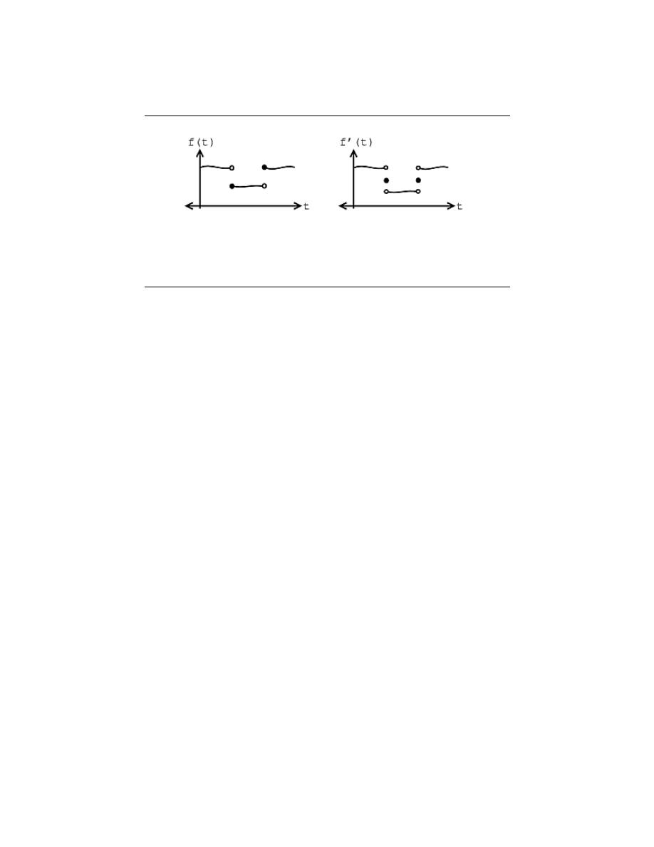
108
CHAPTER 5. FOURIER SERIES
(a)
(b)
Figure 5.20:
Discontinuous functions, f (t).
5.10.2.1 Example
Let us assume we have the following function and equality:
f
0
(t) = lim
N →∞
f
0
N
(t)
(5.48)
If f (t) meets all three conditions of the Strong Dirichlet Conditions, then
f (τ ) = f
0
(τ )
at every τ at which f (t) is continuous. And where f (t) is discontinuous, f
0
(t) is the average
of the values on the right and left. See the figures below as an example:
note:
The functions that fail the Dirchlet conditions are pretty pathological - as
engineers, we are not too interested in them.
6.11 Gibbs’s Phenomena
5.11.1 Introduction
The Fourier Series is the representation of continuous-time, periodic signals in terms of
complex exponentials. The Dirichlet conditions suggest that discontinuous signals may have
a Fourier Series representation so long as there are a finite number of discontinuities. This
seems counter-intuitive, however, as complex exponentials are continuous functions. It does
not seem possible to exactly reconstruct a discontinuous function from a set of continuous
ones. In fact, it is not. However, it can be if we relax the condition of ’exactly’ and replace
it with the idea of ’almost everywhere’. This is to say that the reconstruction is exactly the
same as the original signal except at a finite number of points. These points, not necessarily
suprisingly, occur at the points of discontinuities.
5.11.1.1 History
In the late 1800s, many machines were built to calculate Fourier coefficients and re-synthesize:
f
0
N
(t) =
N
X
n=−N
c
n
e
jω
0
nt
(5.49)

109
Albert Michelson (an extraordinary experimental physicist) built a machine in 1898 that
could compute c
n
up to n = ±79, and he re-synthesized
f
0
79
(t) =
79
X
n=−79
c
n
e
jω
0
nt
(5.50)
The machine performed very well on all tests except those involving discontinuous func-
tions . When a square wave, like that shown in Figure 5.21, was inputed into the machine,
”wiggles” around the discontinuities appeared, and even as the number of Fourier coeffi-
cients approached infinity, the wiggles never disappeared - these can be seen in the last plot
in Figure 5.21. J. Willard Gibbs first explained this phenomenon in 1899, and therefore
these discontinuous points are referred to as Gibbs Phenomenon .
5.11.2 Explanation
We begin this discussion by taking a signal with a finite number of discontinuities (like a
square pulse ) and finding its Fourier Series representation. We then attempt to recon-
struct it from these Fourier coefficients. What we find is that the more coefficients we use,
the more the signal begins to resemble the original. However, around the discontinuities,
we observe rippling that does not seem to subside. As we consider even more coefficients,
we notice that the ripples narrow, but do not shorten. As we approach an infinite number
of coefficients, this rippling still does not go away. This is when we apply the idea of almost
everywhere. While these ripples remain (never dropping below 9% of the pulse height), the
area inside them tends to zero, meaning that the energy of this ripple goes to zero. This
means that their width is approaching zero and we can assert that the reconstruction is
exactly the original except at the points of discontinuity. Since the Dirichlet conditions
assert that there may only be a finite number of discontinuities, we can conclude that the
principle of almost everywhere is met. This phenomenon is a specific case of nonuniform
convergence .
Below we will use the square wave, along with its Fourier Series representation, and show
several figures that reveal this phenomenon more mathematically.
5.11.2.1 Square Wave
The Fourier series representation of a square signal below says that the left and right sides
are ”equal.” In order to understand Gibbs Phenomenon we will need to redefine the way we
look at equality.
s (t) = a
0
+
∞
X
k=1
a
k
cos
2πkt
T
+
∞
X
k=1
b
k
sin
2πkt
T
(5.51)
5.11.2.2 Example
The figure below shows several Fourier series approximation of the square wave using a
varied number of terms, denoted by K:
When comparing the square wave to its Fourier series representation in Figure 5.21, it
is not clear that the two are equal. The fact that the square wave’s Fourier series requires
more terms for a given representation accuracy is not important. However, close inspection
of Figure 5.21 does reveal a potential issue: Does the Fourier series really equal the square
wave at all values of t? In particular, at each step-change in the square wave, the Fourier
series exhibits a peak followed by rapid oscillations. As more terms are added to the series,
the oscillations seem to become more rapid and smaller, but the peaks are not decreasing.
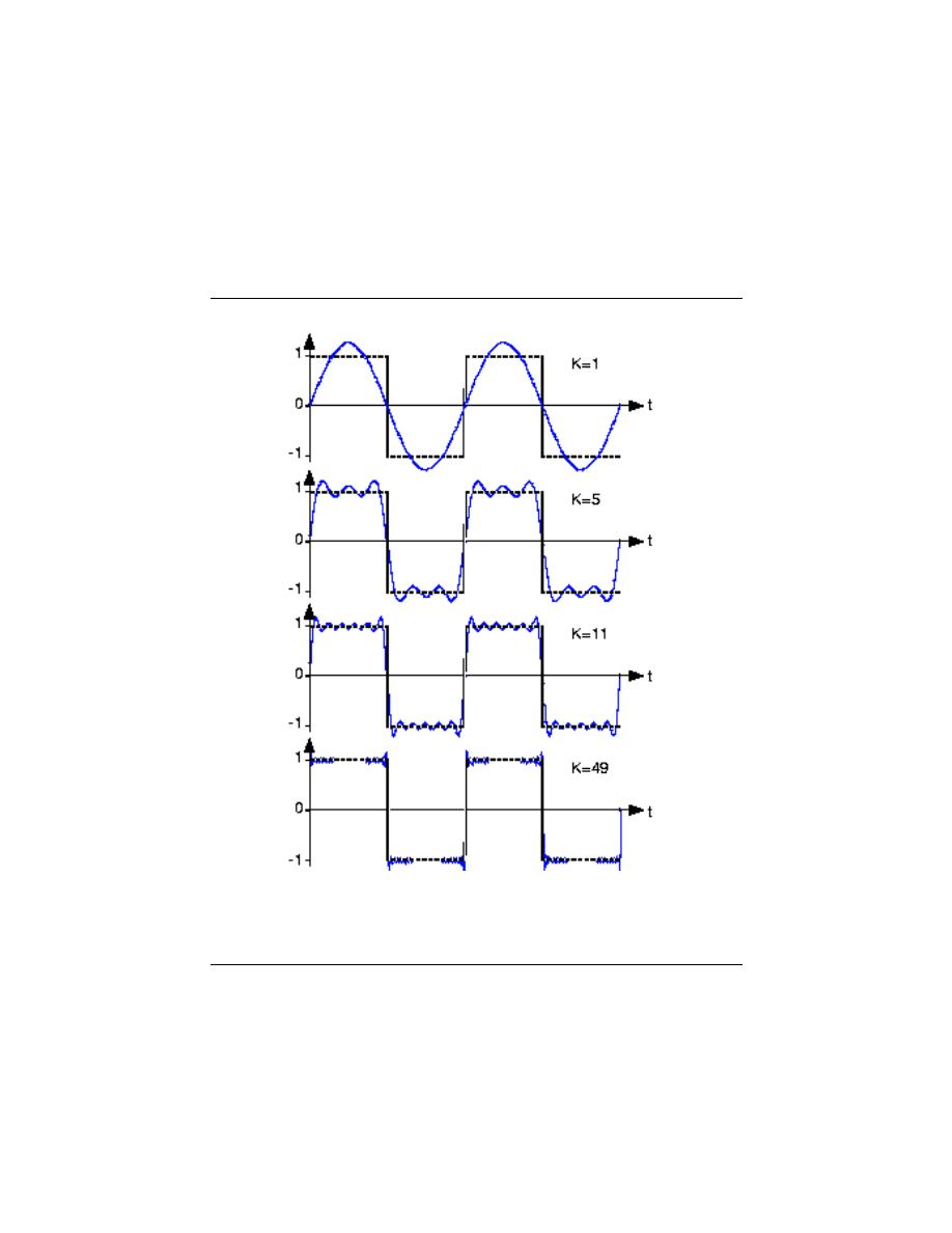
110
CHAPTER 5. FOURIER SERIES
Fourier series approximation of a square wave
Figure 5.21: Fourier series approximation to sq (t). The number of terms in the Fourier
sum is indicated in each plot, and the square wave is shown as a dashed line over two
periods.

111
Consider this mathematical question intuitively: Can a discontinuous function, like the
square wave, be expressed as a sum, even an infinite one, of continuous ones? One should at
least be suspicious, and in fact, it can’t be thus expressed. This issue brought Fourier
3
much
criticism from the French Academy of Science (Laplace, Legendre, and Lagrange comprised
the review committee) for several years after its presentation on 1807. It was not resolved
for also a century, and its resolution is interesting and important to understand from a
practical viewpoint.
The extraneous peaks in the square wave’s Fourier series never disappear; they are
termed Gibb’s phenomenon after the American physicist Josiah Willard Gibbs. They
occur whenever the signal is discontinuous, and will always be present whenever the signal
has jumps.
5.11.2.3 Redefine Equality
Let’s return to the question of equality; how can the equal sign in the definition of the
Fourier series (pg ??) be justified? The partial answer is that pointwise–each and every
value of t–equality is not guaranteed. What mathematicians later in the nineteenth century
showed was that the rms error of the Fourier series was always zero.
lim
K→∞
rms (
K
) = 0
(5.52)
What this means is that the difference between an actual signal and its Fourier series
representation may not be zero, but the square of this quantity has zero integral! It is
through the eyes of the rms value that we define equality: Two signals s
1
(t), s
2
(t) are
said to be equal in the mean square if rms (s
1
− s
2
) = 0. These signals are said to be
equal pointwise if s
1
(t) = s
2
(t) for all values of t. For Fourier series, Gibb’s phenomenon
peaks have finite height and zero width: The error differs from zero only at isolated points–
whenever the periodic signal contains discontinuities–and equals about 9% of the size of the
discontinuity. The value of a function at a finite set of points does not affect its integral.
This effect underlies the reason why defining the value of a discontinuous function at its
discontinuity is meaningless. Whatever you pick for a value has no practical relevance for
either the signal’s spectrum or for how a system responds to the signal. The Fourier series
value ”at” the discontinuity is the average of the values on either side of the jump.
6.12 Fourier Series Wrap-Up
Below we will highlight some of the most important concepts about the Fourier Series and
our understanding of it through eigenfunctions and eigenvalues. Hopefully you are familiar
with all of this material, so this document will simply serve as a refrehser, but if not, then
refer to the many links below for more information on the various ideas and topics.
1. - We can represent a periodic function (or a function on an interval) f (t) as a combi-
nation of complex exponentials:
f (t) =
∞
X
n=−∞
c
n
e
jω
0
nt
(5.53)
c
n
=
1
T
Z
T
0
f (t) e
−(jω
0
nt)
dt
(5.54)
Where the fourier coefficints, c
n
, approximately equal how much of frequency ω
o
n is
in the signal.
3
http://www-groups.dcs.st-and.ac.uk/∼history/Mathematicians/Fourier.html

112
CHAPTER 5. FOURIER SERIES
2. - Since e
jω
0
nt
are eigenfunctions of LTI systems, we can interpret the action of a system
on a signal in terms of its eigenvalues:
H (jω
0
n) =
Z
∞
−∞
h (t) e
−(jω
0
nt)
dt
(5.55)
• - |H (jω
0
n) | is large ⇒ system accentuates frequency ω
0
n
• - |H (jω
0
n) | is small ⇒ system attenuates frequency ω
0
n
3. - In addition, the {c
n
} of a periodic function f (t) can tell us about:
• - symmetries in f (t)
• - smoothness of f (t), where smoothness can be interpretted as the decay rate of
|c
n
|.
4. - We can approximate a function by re-synthesizing using only some of the Fourier
coefficients (truncating the F.S.)
f
0
N
(t) =
X
n≤|N |
c
n
e
jω
0
nt
(5.56)
This approximation works well where f (t) is continuous, but not so well where f (t)
is discontinuous. This idea is explained by Gibb’s Phenomena.

Chapter 6
Hilbert Spaces and Orthogonal
Expansions
7.1 Vector Spaces
6.1.1 Introduction
Much of the language in this section will be familiar to you - you should have previously
been exposed to the concepts of
• - inner products
• - Orthogonality
• - basis expansions
in the context of R
n
. We’re going to take what we know about vectors and apply it to
functions (continuous time signals).
6.1.2 Vector Spaces
Vector space :
A linear vector space S is a collection of ”vectors” such that (1)
if f
1
∈ S ⇒ αf
1
∈ S for all scalars α (where α ∈ R or α ∈ C) and (2) if f
1
∈ S,
f
2
∈ S, then f
1
+ f
2
∈ S
If the scalars α are real, S is called a real vector space .
If the scalars α are complex, S is called a complex vector space .
If the ”vectors” in S are functions of a continuous variable, we sometimes call S a linear
function space
6.1.2.1 Properties
We define a set V to be a vector space if
1. - x + y = y + x for each x and y in V
2. - x + (y + z) = (x + y) + z for each x, y, and z in V
3. - There is a unique ”zero vector” such that x + 0 = x for each x in V
113
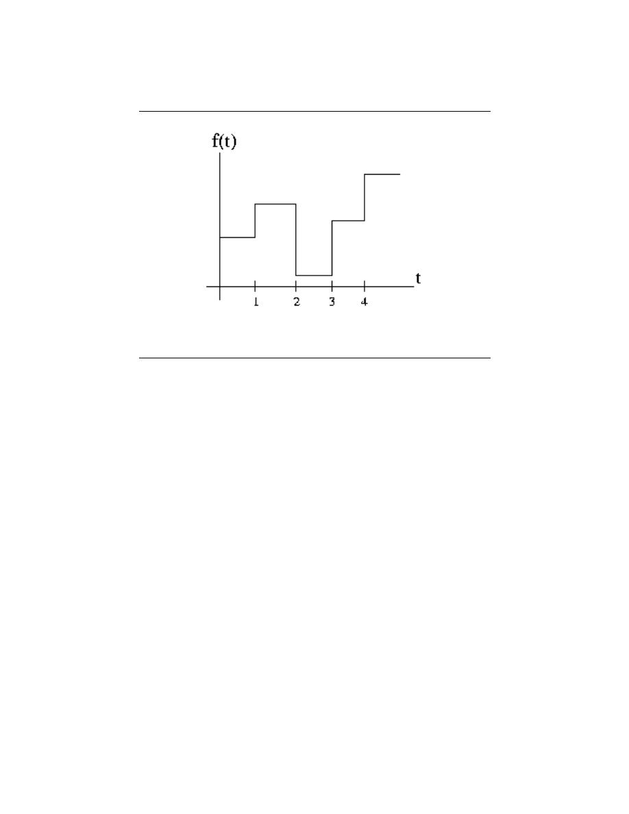
114
CHAPTER 6. HILBERT SPACES AND ORTHOGONAL EXPANSIONS
Figure 6.1
4. - For each x in V there is a unique vector −x such that x + (−x) = 0.
5. - 1x = x
6. - (c
1
c
2
) x = c
1
(c
2
x) for each x in V and c
1
and c
2
in C.
7. - c (x + y) = cx + cy for each x and y in V and c in C.
8. - (c
1
+ c
2
) x = c
1
x + c
2
x for each x in V and c
1
and c
2
in C.
6.1.2.2 Examples
• - R
n
= realvectorspace
• - C
n
= complexvectorspace
• - L
1
(R) =
n
f (t) |
R
∞
−∞
|f (t) |dt < ∞
o
is a vector space
• - L
∞
(R) = { f (t) |f (t) is bounded} is a vector space
• - L
2
(R) =
n
f (t) |
R
∞
−∞
(|f (t) |)
2
dt < ∞
o
= finite energy signals is a vector space
• - L
2
([0, T ]) = finite energy functions on interval [0, T]
• - `
1
(Z), `
2
(Z), `
∞
(Z) are vector spaces
• - The collection of functions piecewise constant between the integers is a vector space
• - R
+
2
=
x
0
x
1
|x
0
> 0 x
1
> 0
is not a vector space.
1
1
∈ R
+
2
, but ∀α, α <
0 : α
1
1
/
∈ R
+
2
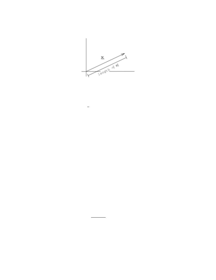
115
Figure 6.2
• - D = {∀z, |z| ≤ 1 : z ∈ C} is not a vector space. z
1
= 1 ∈ D, z
2
= j ∈ D, but
z
1
+ z
2
/
∈ D, |z
1
+ z
2
| =
√
2 > 1
note:
Vector spaces can be collections of functions, collections of sequences, as
well as collections of traditional vectors (i.e. finite lists of numbers)
7.2 Norms
6.2.1 Introduction
Much of the language in this section will be familiar to you - you should have previously
been exposed to the concepts of
• - inner products
• - orthogonality
• - basis expansions
in the context of R
n
. We’re going to take what we know about vectors and apply it to
functions (continuous time signals).
6.2.2 Norms
The norm of a vector is a real number that represents the ”size” of the vector.
Example 6.1:
In R
2
, we can define a norm to be a vectors geometric length.
x = (x
0
, x
1
)
T
, norm k x k=
√
x
0
2
+ x
1
2
Mathematically, a norm k · k is just a function (taking a vector and returning a
real number) that satisfies three rules.
To be a norm, k · k must satisfy:
1. - the norm of every vector is positive ∀x, x ∈ S :k x k> 0
2. - scaling a vector scales the norm by the same amount k αx k= |α| k x k for all vectors
x and scalars α
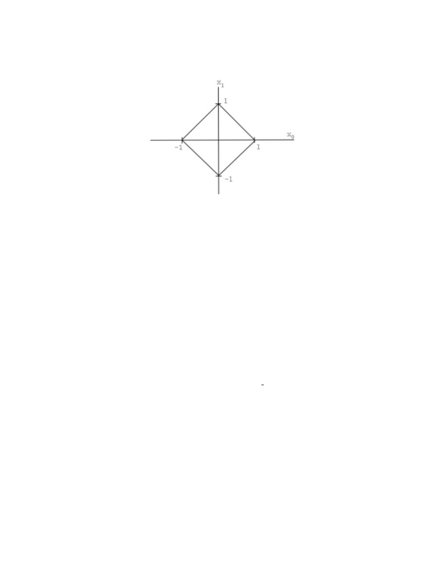
116
CHAPTER 6. HILBERT SPACES AND ORTHOGONAL EXPANSIONS
Figure 6.3: Collection of all x ∈ R
2
with k x k
1
= 1
3. - Triangle Property: k x + y k≤k x k + k y k for all vectors x, y. ”The ”size” of the
sum of two vectors is less than or equal to the sum of their sizes”
A vector space with a well defined norm is called a normed vector space or normed
linear space .
6.2.2.1 Examples
Example 6.2:
R
n
(or C
n
), x =
x
0
x
1
. . .
x
n−1
, k x k
1
=
P
n−1
i=0
(|x
i
|), R
n
with this norm is called
`
1
([0, n − 1]).
Example 6.3:
R
n
(or C
n
), with norm k x k
2
=
P
n−1
i=0
(|x
i
|)
2
1
2
, R
n
is called `
2
([0, n − 1])
(the usual ”Euclidean”norm).
Example 6.4:
R
n
(or C
n
, with norm k x k
∞
= max
i
{|x
i
|} is called `
∞
([0, n − 1])
6.2.2.2 Spaces of Sequences and Functions
We can define similar norms for spaces of sequences and functions.
Discrete time signals = sequences of numbers
x [n] = {. . . , x
−2
, x
−1
, x
0
, x
1
, x
2
, . . . }
• - k x [n] k
1
=
P
∞
i=−∞
(|x [i] |), x [n] ∈ `
1
(Z) ⇒ k x k
1
< ∞
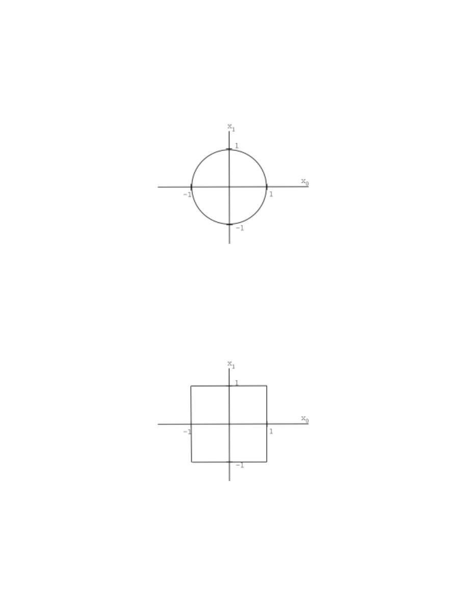
117
Figure 6.4: Collection of all x ∈ R
2
with k x k
2
= 1
Figure 6.5:
x ∈ R
2
with k x k
∞
= 1

118
CHAPTER 6. HILBERT SPACES AND ORTHOGONAL EXPANSIONS
Figure 6.6:
General plot of vectors and angle referred to in above equations.
• - k x [n] k
2
=
P
∞
i=−∞
(|x [i] |)
2
1
2
, x [n] ∈ `
2
(Z) ⇒ k x k
2
< ∞
• - k x [n] k
p
=
P
∞
i=−∞
((|x [i] |)
p
)
1
p
, x [n] ∈ `
p
(Z) ⇒ k x k
p
< ∞
• - k x [n] k
∞
= sup
i
|x [i] |, x [n] ∈ `
∞
(Z) ⇒ k x k
∞
< ∞
For continuous time functions:
• - k f (t) k
p
=
R
∞
−∞
(|f (t) |)
p
dt
1
p
, f (t) ∈ L
p
(R) ⇒ k f (t) k
p
< ∞
• - (On the interval) k f (t) k
p
=
R
T
0
(|f (t) |)
p
dt
1
p
, f (t) ∈ L
p
([0, T ]) ⇒ k f (t) k
p
< ∞
7.3 Inner Products
6.3.1 Definition: Inner Product
You may have run across inner prodcuts , also called dot products , on R
n
before in
some of your math or science courses. If not, we define the inner product as follows, given
we have some x ∈ R
n
and y ∈ R
n
inner product :
The inner product is defined mathematically as:
x · y
=
y
T
x
=
y
0
y
1
. . .
y
n−1
x
0
x
1
..
.
x
n−1
=
P
n−1
i=0
(x
i
y
i
)
(6.1)
6.3.1.1 Inner Product in 2-D
If we have x ∈ R
2
and y ∈ R
2
, then we can write the inner product as
x · y =k x kk y k cos (θ)
(6.2)
where θ is the angle between x and y.
Geometrically, the inner product tells us about the strength of x in the direction of y.
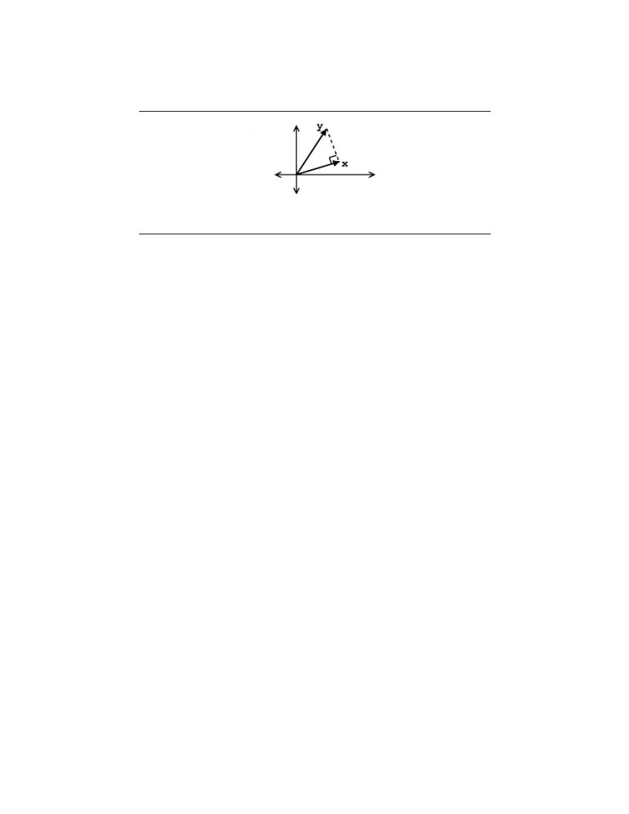
119
Figure 6.7:
Plot of two vectors from above example.
Example 6.5:
For example, if k x k= 1, then
x · y =k y k cos (θ)
The following characteristics are revealed by the inner product:
• - x · y measures the length of the projection of y onto x.
• - x · y is maximum (for given k x k, k y k) when x and y are in the same direction
( θ = 0 ⇒ cos (θ) = 1).
• - x · y is zero when cos (θ) = 0 ⇒ θ = 90
◦
, i.e. x and y are orthogonal .
6.3.1.2 Inner Product Rules
In general, an inner product on a complex vector space is just a function (taking two vectors
and returning a complex number) that satisfies certain rules:
• - Conjugate Symmetry:
x · y = x · y
∗
• - Scaling:
αx · y = αx · y
• - Additivity:
x + y · z = x · z + y · z
• - ”Positivity”:
∀x, x 6= 0 : x · x > 0
orthogonal :
we say that x and y are orthogonal if:
x · y = 0

120
CHAPTER 6. HILBERT SPACES AND ORTHOGONAL EXPANSIONS
7.4 Hilbert Spaces
6.4.1 Hilbert Spaces
A vector space S with a valid inner product defined on it is called an inner product space
, which is also a normed linear space . A Hilbert space is an inner product space
that is complete with respect to the norm defined using the inner product. Hilbert spaces
are named after David Hilbert
1
, who developed this idea through his studies of integral
equations. We define our valid norm using the inner product as:
k x k=
√
x · x
(6.3)
Hilbert spaces are useful in studying and generalizing the concepts of Fourier expansion,
Fourier transforms, and are very important to the study of quantum mechanics. Hilbert
spaces are studied under the functional analysis branch of mathematics.
6.4.1.1 Examples of Hilbert Spaces
Below we will list a few examples of Hilbert spaces. You can verify that these are valid inner
products at home.
• - For C
n
,
x · y = y
T
x =
y
0
∗
y
1
∗
. . .
y
n−1
∗
x
0
x
1
..
.
x
n−1
=
n−1
X
i=0
(x
i
y
i
∗
)
• - Space of finite energy comlpex functions: L
2
(R)
f · g =
Z
∞
−∞
f (t) g (t)
∗
dt
• - Space of square-summable sequences: `
2
(Z)
x · y =
∞
X
i=−∞
x [i] y [i]
∗
7.5 Cauchy-Schwarz Inequality
6.5.1 Introduction
Recall in R
2
, x · y =k x kk y k cos (θ)
|x · y| ≤k x kk y k
(6.4)
The same relation holds for inner product spaces in general...
1
http://www-history.mcs.st-andrews.ac.uk/history/Mathematicians/Hilbert.html

121
6.5.1.1 Cauchy-Schwarz Inequality
Cauchy-Schwarz Inequality :
For x, y in an inner product space
|x · y| ≤k x kk y k
with equality holding if and only if x and y are linearly independent (Section 4.1.1),
i.e. x = αy for some scalar α.
6.5.2 Matched Filter Detector
Also referred to as Cauchy-Schwarz’s ”Killer App.”
6.5.2.1 Concept behind Matched Filter
If we are given two vectors, f and g, then the Cauchy-Schwarz Inequality (CSI) is maximized
when f = αg. This tells us:
• - f is in the same ”direction” as g
• - if f and g are functions, f = αg means f and g have the same shape.
For example, say we are in a situation where we have a set of signals, defined as {g
1
(t) , g
2
(t) , . . . , g
k
(t)},
and we want to be able to tell which, if any, of these signals resemble another given signal
f (t).
strategy: In order to find the signal(s) that resembles f (t) we will take the inner
products. If g
i
(t) resembles f (t), then the absolute value of the inner product,
|f (t) · g
i
(t) |, will be large.
This idea of being able to measure and rank the ”likeness” of two signals leads us to the
Matched Filter Detector .
6.5.2.2 Comparing Signals
The simplest use of the Matched Filter would be to take a set of ”candidate” signals, say
our set of {g
1
(t) , g
2
(t) , . . . , g
k
(t)}, and try to match it to a ”template” signal, f (t). For
example say we are given the below template and candidate signals:
Now if our only question was which function was a closer match to f (t) then we can
easily come up with the answer based on inspection - g
2
(t). However, this will not always
be the case. Also, we may want to develop a method, or algorithm, that could automate
these comparisons. Or perhaps we wish to have a quantitative value expressing just how
simliar the signals are. To address these issues, we will lay out a more formal approach to
comparing the signals, which will, as mentioned above, be based on the inner product.
In order to see which of our candidate signals, g
1
(t) or g
2
(t), best resembles f (t) we
need to perform the following steps:
• - Normalize the g
i
(t)
• - Take the inner product with f (t)
• - Find the biggest!
Or, putting it mathematically:
Bestcandidate = argmax
i
|f · g
i
|
k g
i
k
(6.5)
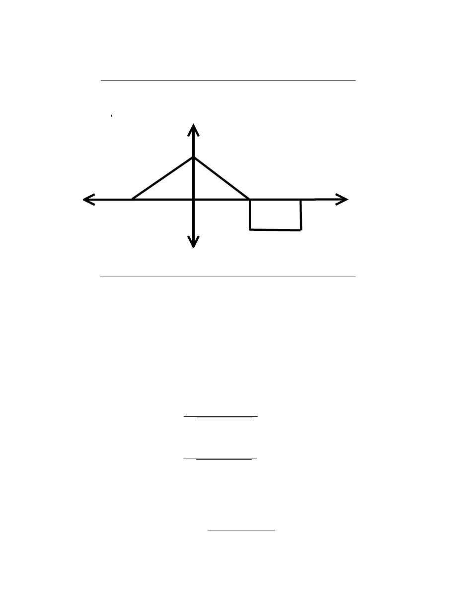
122
CHAPTER 6. HILBERT SPACES AND ORTHOGONAL EXPANSIONS
Template Signal
f(t)
t
Figure 6.8:
Our signal we wish to find match of.
6.5.2.3 Finding a Pattern
Extending these thoughts of using the Matched Filter to find similarities among signals, we
can use the same idea to search for a pattern in a long signal. The idea is simply to repeatedly
perform the same calculation as we did previously; however, now instead of calculating on
different signals we will simply perform the inner product with different shifted versions of
our ”pattern” signal. For example, say we have the following two signals - a pattern signal
and long signal.
Here we will look at two shifts of our pattern signal, shifting the signal by s
1
and s
2
.
These two possibilities yield the following calculations and results:
• - Shift of s
1
:
R
s
1
+T
s
1
g (t) f (t − s
1
) dt
q
R
s
1
+T
s
1
(|g (t) |)
2
dt
= ”large”
(6.6)
• - Shift of s
2
:
R
s
2
+T
s
2
g (t) f (t − s
2
) dt
q
R
s
2
+T
s
2
(|g (t) |)
2
dt
= ”small”
(6.7)
Therefore, we can define a generalized equation for our matched filter:
m (s) = matchedfilter
(6.8)
m (s) =
R
s+T
s
g (t) f (t − s) dt
k g (t) k |
L
2
([s,s+T ])
(6.9)
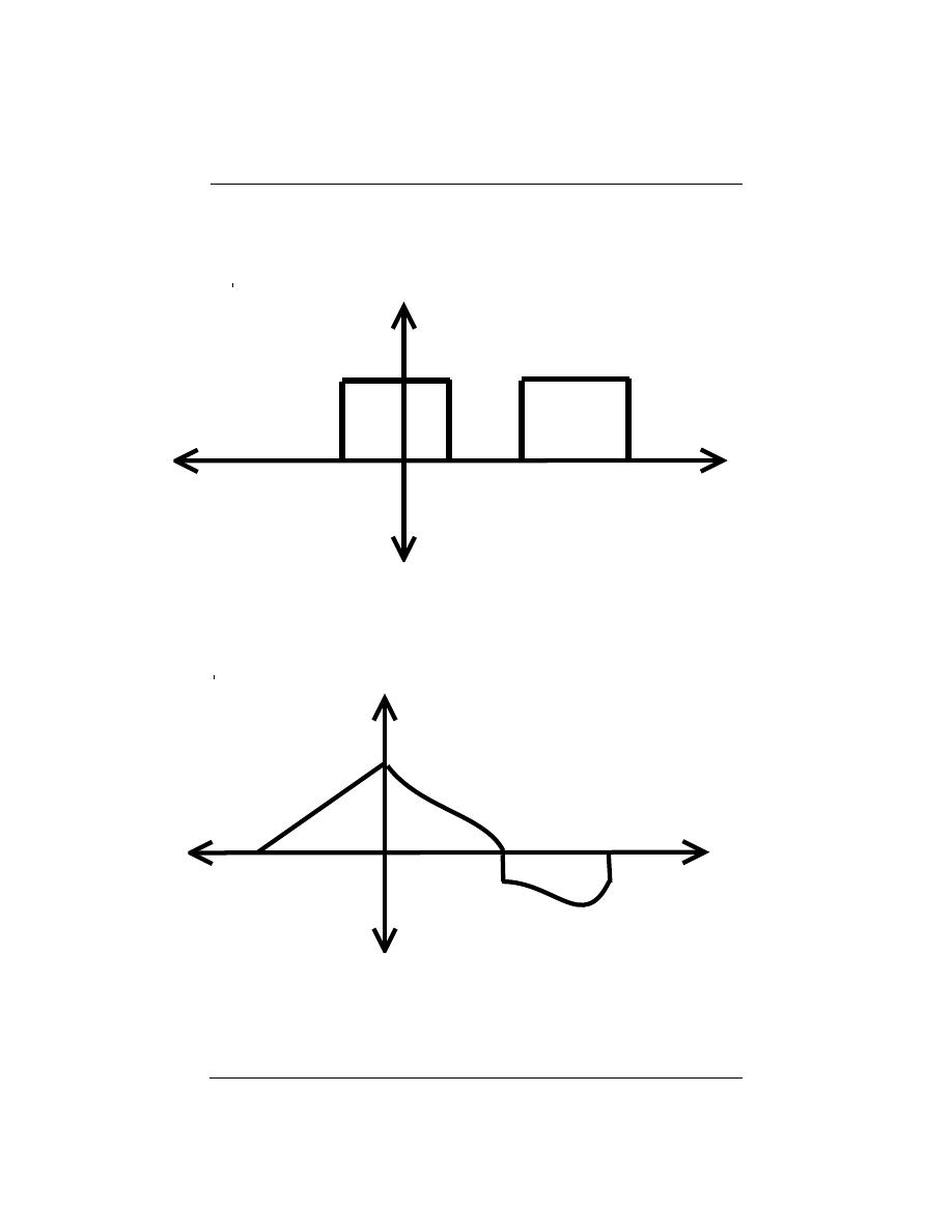
123
Candidate Signals
g (t)
t
1
(a)
g (t)
t
2
(b)
Figure 6.9:
Clearly by looking at these we can see which signal will provide the better
match to our template signal.
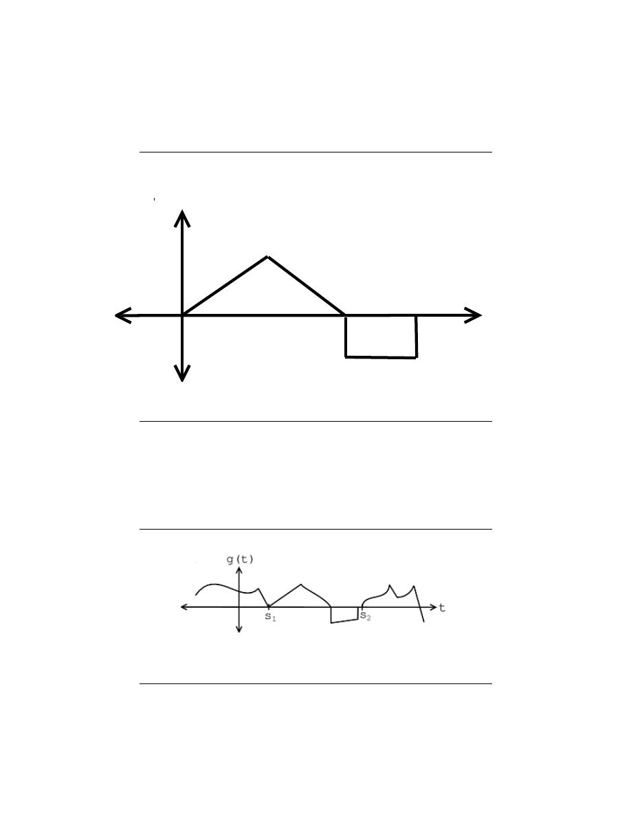
124
CHAPTER 6. HILBERT SPACES AND ORTHOGONAL EXPANSIONS
Pattern Signal
f(t)
t
Figure 6.10:
The pattern we are looking for in a our long signal having a length T .
Long Signal
Figure 6.11:
Here is the long signal that contains a piece that resembles our pattern
signal.

125
(a)
(b)
Figure 6.12:
Example of ”Where’s Waldo?” picture. Our Matched Filter Detector can
be implemented to find a possible match for Waldo.
where the numerator in Equation 6.9 is the convolution of g (t) ∗ f (−t). Now in order to
decide whether or not the result from our matched filter detector is high enough to indicate
an acceptable match between the two signals, we define some threshold . If
m (s
0
) ≥ threshold
then we have a match at location s
0
.
6.5.2.4 Practical Examples
6.5.2.4.1 Image Detection
In 2-D, this concept is used to match images together, such as verifying fingerprints for
security or to match photos of someone. For example, this idea could be used for the
ever-popular ”Where’s Waldo?” books! If we are given the below template and piece of a
”Where’s Waldo?” book,
then we could easily develop a program to find the closest resemblance to the image
of Waldo’s head in the larger picture. We would simply implement our same match filter
algorithm: take the inner products at each shift and see how large our resulting answers
are. This idea was implemented on this same picture for a Signals and Systems Project
2
at
Rice University (click the link to learn more).
2
http://www.owlnet.rice.edu/∼elec301/Projects99/waldo/process.html

126
CHAPTER 6. HILBERT SPACES AND ORTHOGONAL EXPANSIONS
Send:
= ’1’
= ’0’
Figure 6.13:
Frequency Shift Keying for ’1’ and ’0’.
6.5.2.4.2 Communications Systems
Matched filter detector are also commonly used in Communications Systems. In fact, they
are the optimal detectors in Gaussian noise. Signals in the real-world are often distorted by
the environment around them, so there is a constant struggle to develop ways to be able to
receive a distorted signal and then be able to filter it in some way to determine what the
original signal was. Matched filters provide one way to compare a received signal with two
possible original (”template”) signals and determine which one is the closest match to the
received signal.
For example, below we have a simplified example of Frequency Shift Keying (FSK) where
we having the following coding for ’1’ and ’0’:
Based on the above coding, we can create digital signals based on 0’s and 1’s by putting
together the above two ”codes” in an infinite number of ways. For this example we will
transmit a basic 3-bit number, 101, which is displayed in the following figure:
Now, the signal picture aboved represents our original signal that will be transmitted over
some commmuncication system, which will inevitably pass through the ”communications
channel,” the part of the system that will distort and alter our signal. As long as the noise
is not too great, our matched filter should keep us from having to worry about these changes
to our transmitted signal. Once this signal has been received, we will pass the noisy signal
through a simple system, simliar to the simplified version shown below:
The above diagram basical shows that our noisy signal will be passed in (we will assume
that it passes in one ”bit” at a time) and this signal will be split and passed to two different
matched filter detectors. Each one will compare the noisy, received signal to one of the two
codes we defined for ’1’ and ’0.’ Then this value will be passed on and whichever value is
higher (i.e. whichever FSK code signal the noisy signal most resembles) will be the value
that the receiver takes. For example, the first bit that will be sent through will be a ’1’ so
the upper level of the block diagram will have a higher value, thus denoting that a ’1’ was
sent by the signal, even though the signal may appear very noisy and distorted.
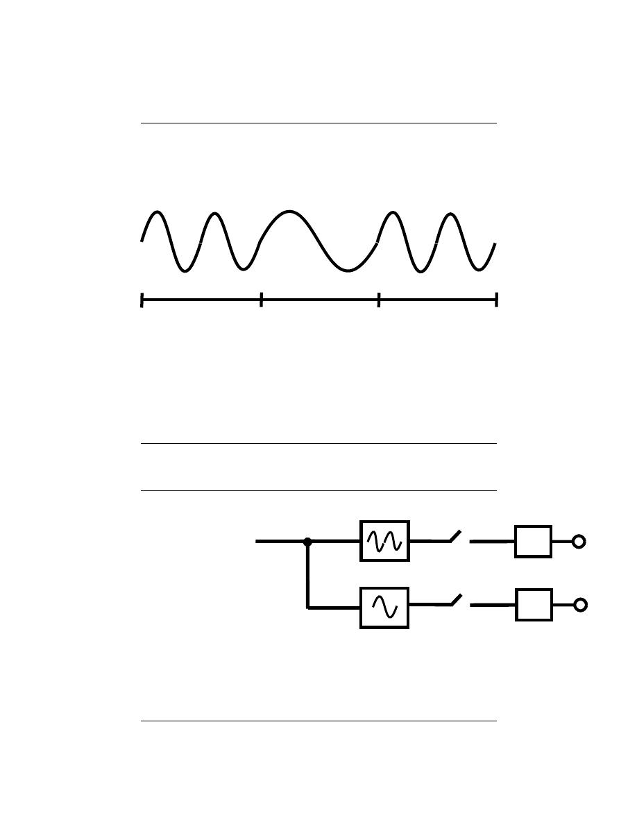
127
1
1
0
asdfasd
asdfasd
Figure 6.14:
The bit stream ”101” coded with the above FSK.
Noisy
Signal
Input
Choose
Max
(.)
(.)
Matched
Filters
Figure 6.15:
Block diagram of matched filter detector.

128
CHAPTER 6. HILBERT SPACES AND ORTHOGONAL EXPANSIONS
6.5.3 Proof of CSI
Here will look at the proof of our Cauchy-Schwarz Inequality (CSI) for a real vector space
.
Theorem 6.1:
CSI for Real Vector Space
For f ∈ HilbertSpaceS and g ∈ HilbertSpaceS, show:
|f · g| ≤k f kk g k
(6.10)
with equality if and only if g = αf .
Proof:
•- If g = αf , show |f · g| =k f kk g k
|f · g| = |f · αf | = |α||f · f | = |α|(k f k)
2
|f · g| =k f k (|α| k f k) =k f kk g k
This verifies our above statement of the CSI!
•- If g 6= αf , show |f · g| <k f kk g k where we have ∀β, β ∈ R : βf + g 6= 0
0 < (k βf + g k)
2
= βf + g · βf + g = β
2
f · f + 2βf · g + g · g
= β
2
(k f k)
2
+ 2βf · g + (k g k)
2
And we get a quadritic in β. Visually, the quadratic polynomial in β > 0 forall
β. Also, note that this polynomial has no real roots and the discriminant is
less than 0. - BLAH BLAH BLAH –
aβ
2
+ bβ + c
has discriminant β
2
− 4ac where we have:
a = (k f k)
2
b = 2f · g
c = (k g k)
2
Therefore, we can plug this values into the above polynomials discriminant to
get:
4(|f · g|)
2
− 4(k f k)
2
(k g k)
2
< 0
(6.11)
|f · g| <k f kk g k
(6.12)
And finally we have proven the Cauchy-Schwarz Inequality formula for real
vectors spaces.
question:
What changes do we have to make to the proof for a
complex vector space? (try to figure this out at home)
7.6 Common Hilbert Spaces
6.6.1 Common Hilbert Spaces
Below we will look at the four most common Hilbert spaces that you will have to deal with
when discussing and manipulating signals and systems.

129
6.6.1.1
R
n
(reals scalars) and C
n
(complex scalars), also called `
2
([0, n − 1])
x =
x
0
x
1
. . .
x
n−1
is a list of numbers (finite sequence). The inner product for our two
spaces are as follows:
• - Inner product R
n
:
x · y
=
y
T
x
=
P
n−1
i=0
(x
i
y
i
)
(6.13)
• - Inner product C
n
:
x · y
=
y
T ∗
x
=
P
n−1
i=0
(x
i
y
i
∗
)
(6.14)
Model for: Discrete time signals on the interval [0, n − 1] or Periodic (with period n)
discrete time signals.
x
0
x
1
. . .
x
n−1
6.6.1.2
f ∈ L
2
([a, b]) is a finite energy function on [a, b]
Inner Product
f · g =
Z
b
a
f (t) g (t)
∗
dt
(6.15)
Model for: continuous time signals on the interval [a, b] or Periodic (with period T = b − a)
continuous time signals
6.6.1.3
x ∈ `
2
(Z) is an infinite sequence of numbers that’s square-summable
Inner product
x · y =
∞
X
i=−∞
x [i] y [i]
∗
(6.16)
Model for: discrete time, non-periodic signals
6.6.1.4
f ∈ L
2
(R) is a finite energy function on all of R.
Inner product
f · g =
Z
∞
−∞
f (t) g (t)
∗
dt
(6.17)
Model for: continuous time, non-periodic signals

130
CHAPTER 6. HILBERT SPACES AND ORTHOGONAL EXPANSIONS
Figure 6.16

131
6.6.2 Associated Fourier Analysis
Each of these 4 Hilbert spaces has a type of Fourier analysis associated with it.
• - L
2
([a, b]) → Fourier series
• - `
2
([0, n − 1]) → Discrete Fourier Transform
• - L
2
(R) → Fourier Transform
• - `
2
(Z) → Discrete Time Fourier Transform
But all 4 of these are based on the same principles (Hilbert space).
Important note:
Not all normed spaces are Hilbert spaces
For example: L
1
(R), k f k
1
=
R |f (t) |dt. Try as you might, you can’t find an inner product
that induces this norm, i.e. a · · · such that
f · f
=
R (|f (t) |)
2
dt
2
=
k f k
1
2
(6.18)
In fact, of all the L
p
(R) spaces, L
2
(R) is the only one that is a Hilbert space.
Hilbert spaces are by far the nicest. If you use or study orthonormal basis expansion
then you will start to see why this is true.
7.7 Types of Basis
6.7.1 Normalized Basis
Normalized Basis :
a basis (Section 4.1.3) {b
i
} where each b
i
has unit norm
∀i, i ∈ Z :k b
i
k= 1
(6.19)
note:
The concept of basis applies to all vector spaces. The concept of normal-
ized basis applies only to normed spaces.
You can always normalize a basis: just multiply each basis vector by a constant, such as
1
kb
i
k
Example 6.6:
We are given the following basis:
{b
0
, b
1
} =
1
1
,
1
−1
Normalized with `
2
norm:
˜
b
0
=
1
√
2
1
1
˜
b
1
=
1
√
2
1
−1
Normalized with `
1
norm:
˜
b
0
=
1
2
1
1
˜
b
1
=
1
2
1
−1
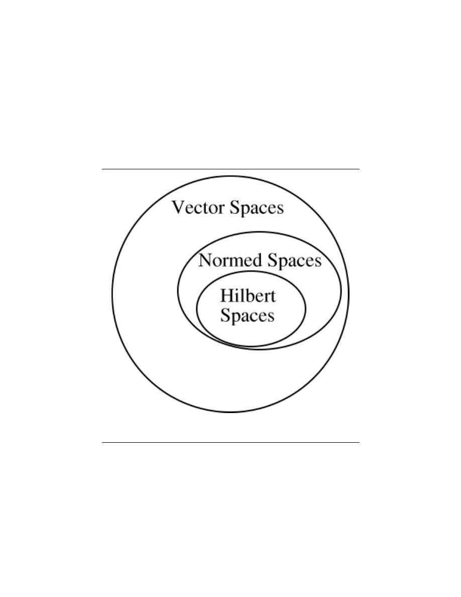
132
CHAPTER 6. HILBERT SPACES AND ORTHOGONAL EXPANSIONS
Figure 6.17

133
6.7.2 Orthogonal Basis
Orthogonal Basis :
a basis {b
i
} in which the elements are mutually orthog-
onal
∀i, i 6= j : b
i
· b
j
= 0
note:
The concept of orthogonal basis applies only to Hilbert Spaces (pg ??).
Example 6.7:
Standard basis for R
2
, also referred to as `
2
([0, 1]):
b
0
=
1
0
b
1
=
0
1
b
0
· b
1
=
1
X
i=0
(b
0
[i] b
1
[i]) = 1 × 0 + 0 × 1 = 0
Example 6.8:
Now we have the following basis and relationship:
1
1
,
1
−1
= {h
0
, h
1
}
h
0
· h
1
= 1 × 1 + 1 × (−1) = 0
6.7.3 Orthonormal Basis
Pulling the previous two sections (definitions) together, we arrive at the most important
and useful basis type:
Orthonormal Basis :
a basis that is both normalized and orthogonal
∀i, i ∈ Z :k b
i
k= 1
∀i, i 6= j : b
i
· b
j
notation:
We can shorten these two statements into one:
b
i
· b
j
= δ
ij
where
δ
ij
=
1 if i = j
0 if i 6= j
Where δ
ij
is referred to as the Kronecker delta function and is also often written
as δ [i − j].
Example 6.9:
Orthonormal Basis Example #1
{b
0
, b
2
} =
1
0
,
0
1

134
CHAPTER 6. HILBERT SPACES AND ORTHOGONAL EXPANSIONS
Example 6.10:
Orthonormal Basis Example #2
{b
0
, b
2
} =
1
1
,
1
−1
Example 6.11:
Orthonormal Basis Example #3
{b
0
, b
2
} =
1
√
2
1
1
,
1
√
2
1
−1
6.7.3.1 Beauty of Orthonormal Bases
Orthonormal bases are very easy to deal with! If {b
i
} is an orthonormal basis, we can write
for any x
x =
X
i
(α
i
b
i
)
(6.20)
It is easy to find the α
i
:
x · b
i
=
P
k
(α
k
b
k
) · b
i
=
P
k
(α
k
b
k
· b
i
)
(6.21)
where in the above equation we can use our knowledge of the delta function to reduce this
equation:
b
k
· b
i
= δ
ik
=
1 if i = k
0 if i 6= k
x · b
i
= α
i
(6.22)
Therefore, we can conclude the following important equation for x:
x =
X
i
(x · b
i
b
i
)
(6.23)
The α
i
’s are easy to compute (no interaction between the b
i
’s)
Example 6.12:
Given the following basis:
{b
0
, b
1
} =
1
√
2
1
1
,
1
√
2
1
−1
represent x =
3
2
Example 6.13:
Slightly Modified Fourier Series
We are given the basis
1
√
T
e
jω
0
nt
|
∞
n=−∞
on L
2
([0, T ]) where T =
2π
ω
0
.
f (t) =
∞
X
n=−∞
f · e
jω
0
nt
e
jω
0
nt
1
√
T
Where we can calculate the above inner product in L
2
as
f · e
jω
0
nt
=
1
√
T
Z
T
0
f (t) e
jω
0
nt∗
dt =
1
√
T
Z
T
0
f (t) e
−(jω
0
nt)
dt

135
6.7.3.2 Orthonormal Basis Expansions in a Hilbert Space
Let {b
i
} be an orthonormal basis for a Hilbert space H. Then, for any x ∈ H we can write
x =
X
i
(α
i
b
i
)
(6.24)
where α
i
= x · b
i
.
• - ”Analysis”: decomposing x in term of the b
i
α
i
= x · b
i
(6.25)
• - ”Synthesis”: building x up out of a weighted combination of the b
i
x =
X
i
(α
i
b
i
)
(6.26)
7.8 Orthonormal Basis Expansions
6.8.1 Main Idea
When working with signals many times it is helpful to break up a signal into smaller, more
manageable parts. Hopefully by now you have been exposed to the concept of eigenvectors
and there use in decomposing a signal into one of its possible basis. By doing this we are able
to simplify our calculations of signals and systems through eigenfunctions of LTI systems.
Now we would like to look at an alternative way to represent signals, through the use
of orthonormal basis . We can think of orthonormal basis as a set of building blocks we
use to construct functions. We will build up the signal/vector as a weighted sum of basis
elements.
Example 6.14:
The complex sinusoids
1
√
T
e
jω
0
nt
forall −∞ < n < ∞ form an orthonormal basis
for L
2
([0, T ]).
In our Fourier series equation, f (t) =
P
∞
n=−∞
c
n
e
jω
0
nt
, the {c
n
} are just another
representation of f (t).
note:
For signals/vectors in a Hilbert Space (pg ??), the expansion coefficients
are easy to find.
6.8.2 Alternate Representation
Recall our definition of a basis : A set of vectors {b
i
} in a vector space S is a basis if
1. - The b
i
are linearly independent.
2. - The b
i
span (Section 4.1.2) S. That is, we can find {α
i
}, where α
i
∈ C (scalars) such
that
∀x, x ∈ S : x =
X
i
(α
i
b
i
)
(6.27)
where x is a vector in S, α is a scalar in C, and b is a vector in S.
Condition 2 in the above definition says we can decompose any vector in terms of the
{b
i
}. Condition 1 ensures that the decomposition is unique (think about this at home).

136
CHAPTER 6. HILBERT SPACES AND ORTHOGONAL EXPANSIONS
note:
The {α
i
} provide an alternate representation of x.
Example 6.15:
Let us look at simple example in R
2
, where we have the following vector:
x =
1
2
Standard Basis: {e
0
, e
1
} =
n
(1, 0)
T
, (0, 1)
T
o
x = e
0
+ 2e
1
Alternate Basis: {h
0
, h
1
} =
n
(1, 1)
T
, (1, −1)
T
o
x =
3
2
h
0
+
−1
2
h
1
In general, given a basis {b
0
, b
1
} and a vector x ∈ R
2
, how do we find the α
0
and α
1
such that
x = α
0
b
0
+ α
1
b
1
(6.28)
6.8.3 Finding the Alphas
Now let us address the question posed above about finding α
i
’s in general for R
2
. We start
by rewriting Equation 6.28 so that we can stack our b
i
’s as columns in a 2×2 matrix.
x
= α
0
b
0
+ α
1
b
1
(6.29)
x
=
..
.
..
.
b
0
b
1
..
.
..
.
α
0
α
1
(6.30)
Example 6.16:
Here is a simple example, which shows a little more detail about the above equa-
tions.
x [0]
x [1]
=
α
0
b
0
[0]
b
0
[1]
+ α
1
b
1
[0]
b
1
[1]
=
α
0
b
0
[0] + α
1
b
1
[0]
α
0
b
0
[1] + α
1
b
1
[1]
(6.31)
x [0]
x [1]
=
b
0
[0]
b
1
[0]
b
0
[1]
b
1
[1]
α
0
α
1
(6.32)
6.8.3.1 Simplifying our Equation
To make notation simpler, we define the following two items from the above equations:
• - Basis Matrix :
B =
..
.
..
.
b
0
b
1
..
.
..
.

137
• - Coefficient Vector :
α =
α
0
α
1
This gives us the following, concise equation:
x = Bα
(6.33)
which is equivalent to x =
P
1
i=0
(α
i
b
i
).
Example 6.17:
Given a standard basis,
1
0
,
0
1
, then we have the following basis ma-
trix:
B =
0
1
1
0
To get the α
i
’s, we solve for the coefficient vector in Equation 6.33
α = B
−1
x
(6.34)
Where B
−1
is the inverse matrix of B.
6.8.3.2 Examples
Example 6.18:
Let us look at the standard basis first and try to calculate α from it.
B =
1
0
0
1
= I
Where I is the identity matrix . In order to solve for α let us find the inverse of
B first (which is obviously very trivial in this case):
B
−1
=
1
0
0
1
Therefore we get,
α = B
−1
x = x
Example 6.19:
Let us look at a ever-so-slightly more complicated basis of
1
1
,
1
−1
=
{h
0
, h
1
} Then our basis matrix and inverse basis matrix becomes:
B =
1
1
1
−1
B
−1
=
1
2
1
2
1
2
−1
2
and for this example it is given that
x =
3
2

138
CHAPTER 6. HILBERT SPACES AND ORTHOGONAL EXPANSIONS
Now we solve for α
α = B
−1
x =
1
2
1
2
1
2
−1
2
3
2
=
2.5
0.5
and we get
x = 2.5h
0
+ 0.5h
1
Exercise 6.1:
Now we are given the following basis matrix and x:
{b
0
, b
1
} =
1
2
,
3
0
x =
3
2
For this problem, make a sketch of the bases and then represent x in terms of b
0
and b
1
.
Solution:
In order to represent x in terms of b
0
and b
1
we will follow the same steps we used
in the above example.
B =
1
2
3
0
B
−1
=
0
1
2
1
3
−1
6
α = B
−1
x =
1
2
3
And now we can write x in terms of b
0
and b
1
.
x = b
0
+
2
3
b
1
And we can easily substitute in our known values of b
0
and b
1
to verify our results.
note:
A change of basis simply looks at x from a ”different perspective.” B
−1
transforms x from the standard basis to our new basis, {b
0
, b
1
}. Notice that this
is a totally mechanical procedure.
6.8.4 Extending the Dimension and Space
We can also extend all these ideas past just R
2
and look at them in R
n
and C
n
. This
procedure extends naturally to higher (>2) dimensions. Given a basis {b
0
, b
1
, . . . , b
n−1
} for
R
n
, we want to find {α
0
, α
1
, . . . , α
n−1
} such that
x = α
0
b
0
+ α
1
b
1
+ · · · + α
n−1
b
n−1
(6.35)
Again, we will set up a basis matrix
B =
b
0
b
1
b
2
. . .
b
n−1

139
where the columns equal the basis vectors and it will always be an n×n matrix (although
the above matrix does not appear to be square since we left terms in vector notation). We
can then proceed to rewrite Equation 6.33
x =
b
0
b
1
. . .
b
n−1
α
0
..
.
α
n−1
= Bα
and
α = B
−1
x
7.9 Function Space
We can also find basis vectors for vector spaces other than R
n
.
Let P
n
be the vector space of n-th order polynomials on (-1, 1) with real coefficients
(verify P
2
is a v.s. at home).
Example 6.20:
P
2
= {all quadratic polynomials}. Let b
0
(t) = 1, b
1
(t) = t, b
2
(t) = t
2
.
{b
0
(t) , b
1
(t) , b
2
(t)} span P
2
, i.e. you can write any f (t) ∈ P
2
as
f (t) = α
0
b
0
(t) + α
1
b
1
(t) + α
2
b
2
(t)
for some α
i
∈ R.
Note:
P
2
is 3 dimensional.
f (t) = t
2
− 3t − 4
Alternate basis
{b
0
(t) , b
1
(t) , b
2
(t)} =
1, t,
1
2
3t
2
− 1
write f(t) in terms of this new basis d
0
(t) = b
0
(t), d
1
(t) = b
1
(t), d
2
(t) =
3
2
b
2
(t) −
1
2
b
0
(t).
f (t) = t
2
− 3t − 4 = 4b
0
(t) − 3b
1
(t) + b
2
(t)
f (t) = β
0
d
0
(t) + β
1
d
1
(t) + β
2
d
2
(t) = β
0
b
0
(t) + β
1
b
1
(t) + β
2
3
2
b
2
(t) −
1
2
b
0
(t)
f (t) =
β
0
−
1
2
b
0
(t) + β
1
b
1
(t) +
3
2
β
2
b
2
(t)
so
β
0
−
1
2
= 4
β
1
= −3
3
2
β
2
= 1
then we get
f (t) = 4.5d
0
(t) − 3d
1
(t) +
2
3
d
2
(t)

140
CHAPTER 6. HILBERT SPACES AND ORTHOGONAL EXPANSIONS
Example 6.21:
e
jω
0
nt
|
∞
n=−∞
is a basis for L
2
([0, T ]), T =
2π
ω
0
, f (t) =
P
n
C
n
e
jω
0
nt
.
We calculate the expansion coefficients with
”change of basis” formula
C
n
=
1
T
Z
T
0
f (t) e
−(jω
0
nt)
dt
(6.36)
note:
There are an infinite number of elments in the basis set, that
means L
2
([0, T ]) is infinite dimensional (scary!)
Infinite-dimensional spaces are hard to visualize. We can get a handle on the
intuition by recognizing they share many of the same mathematical properties with
finite dimensional spaces. Many concepts apply to both (like ”basis expansion”).
Some don’t (change of basis isn’t a nice matrix formula).
7.10 Haar Wavelet Basis
6.10.1 Introduction
Fourier series is a useful orthonormal representation on L
2
([0, T ]) especiallly for inputs into
LTI systems. However, it is ill suited for some applications, i.e. image processing (recall
Gibb’s phenomena).
Wavelets , discovered in the last 15 years, are another kind of basis for L
2
([0, T ]) and
have many nice properties.
6.10.2 Basis Comparisons
Fourier series - c
n
give frequency information. Basis functions last the entire interval.
Wavelets - basis functions give frequency info but are local in time.
In Fourier basis, the basis functions are harmonic multiples of e
jω
0
t
In Haar wavelet basis, the basis functions are scaled and translated versions of a ”mother
wavelet” ψ (t).
Basis functions {ψ
j,k
(t)} are indexed by a scale j and a shift k.
Let ∀, 0 ≤ t < T : φ (t) = 1 Then
n
φ (t) , 2
j
2
ψ 2
j
t − k
|j ∈ Z k = 0, 1, 2, . . . , 2
j
− 1
o
ψ (t) =
1 if 0 ≤ t <
T
2
−1 if 0 ≤
T
2
< T
(6.37)
Let ψ
j,k
(t) = 2
j
2
ψ 2
j
t − k
Larger j → ”skinnier” basis function, j = {0, 1, 2, . . . }, 2
j
shifts at each scale: k =
0, 1, . . . , 2
j
− 1
Check: each ψ
j,k
(t) has unit energy
Z
ψ
j,k
2
(t) dt = 1 ⇒ k ψ
j,k
(t) k
2
= 1
(6.38)
Any two basis functions are orthogonal.
Also, {ψ
j,k
, φ} span L
2
([0, T ])

141
Figure 6.18: Fourier basis functions

142
CHAPTER 6. HILBERT SPACES AND ORTHOGONAL EXPANSIONS
Figure 6.19: Wavelet basis functions
Figure 6.20:
basis =
n
1
√
T
e
jω
0
nt
o

143
Figure 6.21
6.10.3 Haar Wavelet Transform
Using what we know about Hilbert spaces: For any f (t) ∈ L
2
([0, T ]), we can write
Synthesis
f (t) =
X
j
X
k
(w
j,k
ψ
j,k
(t))
!
+ c
0
φ (t)
(6.39)
Analysis
w
j,k
=
Z
T
0
f (t) ψ
j,k
(t) dt
(6.40)
c
0
=
Z
T
0
f (t) φ (t) dt
(6.41)
note:
the w
j,k
are real
The Haar transform is super useful especially in image compression
7.11 Orthonormal Bases in Real and Complex Spaces
6.11.1 Notation
Transpose operator A
T
flips the matrix across it’s diagonal.
A =
a
1,1
a
1,2
a
2,1
a
2,2
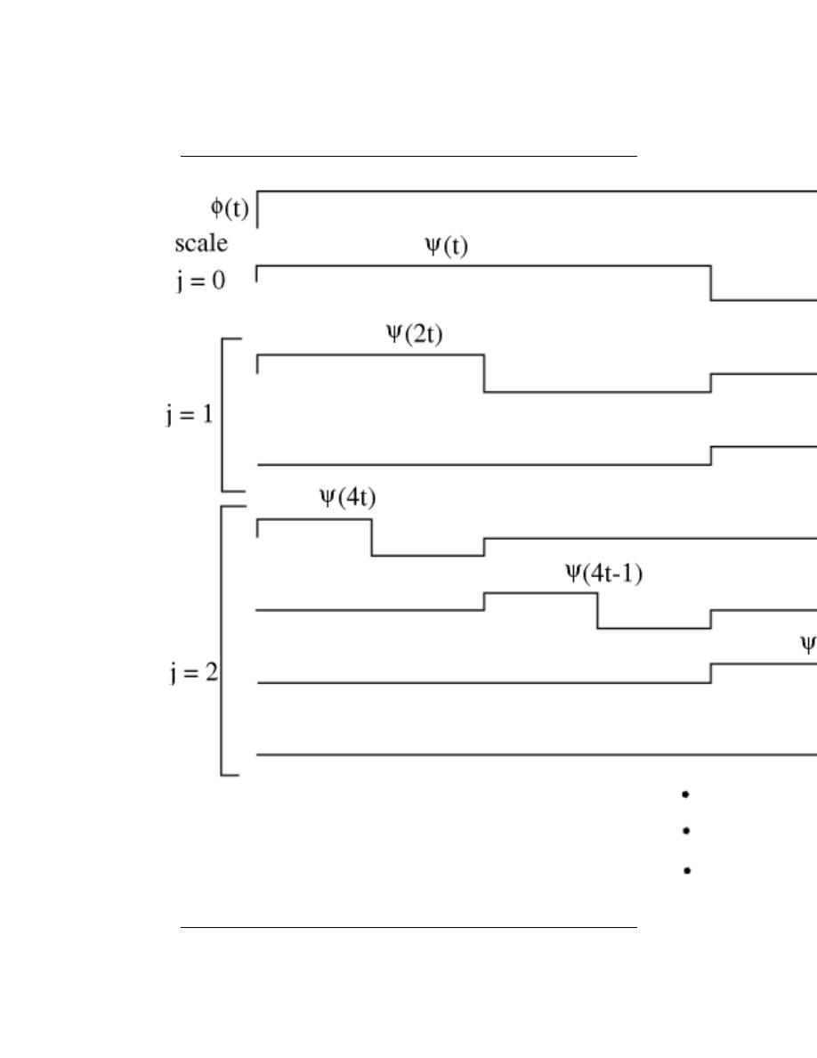
144
CHAPTER 6. HILBERT SPACES AND ORTHOGONAL EXPANSIONS
Figure 6.22
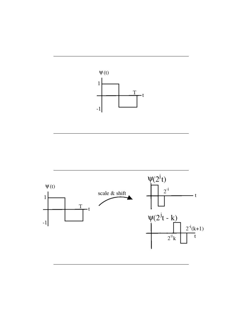
145
Figure 6.23
Figure 6.24
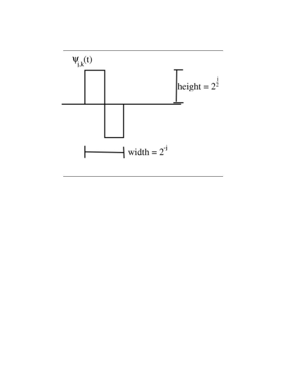
146
CHAPTER 6. HILBERT SPACES AND ORTHOGONAL EXPANSIONS
Figure 6.25
A
T
=
a
1,1
a
2,1
a
1,2
a
2,2
Column i of A is row i of A
T
Recall, inner product
x =
x
0
x
1
..
.
x
n−1
y =
y
0
y
1
..
.
y
n−1
x
T
y =
x
0
x
1
. . .
x
n−1
y
0
y
1
..
.
y
n−1
=
X
(x
i
y
i
) = y · x
on R
n
Hermitian transpose A
H
, transpose and conjugate
A
H
= A
T ∗
y · x = x
H
y =
X
(x
i
y
i
∗
)

147
(a)
(b)
Figure 6.26: Integral of product = 0 (a) Same scale (b) Different scale

148
CHAPTER 6. HILBERT SPACES AND ORTHOGONAL EXPANSIONS
on C
n
Now, let {b
0
, b
1
, . . . , b
n−1
} be an orthonormal basis (Section 6.7.3) for C
n
∀i, : i = {0, 1, . . . , n − 1} b
i
· b
i
= 1
i 6= jb
i
· b
j
= b
j
H
b
i
= 0
Basis matrix:
B =
..
.
..
.
..
.
b
0
b
1
. . .
b
n−1
..
.
..
.
..
.
Now,
B
H
B =
. . .
b
0
H
. . .
. . .
b
1
H
. . .
..
.
. . .
b
n−1
H
. . .
..
.
..
.
..
.
b
0
b
1
. . .
b
n−1
..
.
..
.
..
.
=
b
0
H
b
0
b
0
H
b
1
. . .
b
0
H
b
n−1
b
1
H
b
0
b
1
H
b
1
. . .
b
1
H
b
n−1
..
.
b
n−1
H
b
0
b
n−1
H
b
1
. . .
b
n−1
H
b
n−1
For orthonormal basis with basis matrix B
B
H
= B
−1
( B
T
= B
−1
in R
n
) B
H
is easy to calculate while B
−1
is hard to calculate.
So, to find {α
0
, α
1
, . . . , α
n−1
} such that
x =
X
(α
i
b
i
)
Calculate
α = B
−1
x ⇒ α = B
H
x
Using an orthonormal basis we rid ourselves of the inverse operation.
7.12 Plancharel and Parseval’s Theorems
6.12.1 Plancharel Theorem
Theorem 6.2:
Plancharel Theorem
The inner product of two vectors/signals is the same as the `
2
inner product of
their expansion coefficients.
Let {b
i
} be an orthonormal basis for a Hilbert Space H. x ∈ H, y ∈ H
x =
X
(α
i
b
i
)
y =
X
(β
i
b
i
)
then
x · y
H
=
X
(α
i
β
i
∗
)

149
Example 6.22:
Applying the Fourier Series, we gan go from f (t) to {c
n
} and g (t) to
{d
n
}
Z
T
0
f (t) g (t)
∗
dt =
∞
X
n=−∞
(c
n
d
n
∗
)
inner product in time-domain = inner product of Fourier coefficients
Proof:
x =
X
(α
i
b
i
)
y =
X
(β
j
b
j
)
x · y
H
=
X
(α
i
b
i
) ·
X
(β
j
b
j
) =
X
α
i
b
i
·
X
(β
j
b
j
) =
X
α
i
X
(β
j
∗
)
b
i
· b
j
=
X
(α
i
β
i
∗
)
by using inner product rules (pg 119)
note:
b
i
· b
j
= 0 when i 6= j and b
i
· b
j
= 1 when i = j
If Hilbert space H has a ONB, then inner products are equivalent to inner products
in `
2
.
All H with ONB are somehow equivalent to `
2
.
point of interest:
square-summable sequences are important
6.12.2 Parseval’s Theorem
Theorem 6.3:
Parseval’s Theorem
Energy of a signal = sum of squares of it’s expansion coefficients
Let x ∈ H, {b
i
} ONB
x =
X
(α
i
b
i
)
Then
(k x k
H
)
2
=
X
(|α
i
|)
2
Proof:
Directly from Plancharel
(k x k
H
)
2
= x · x
H
=
X
(α
i
α
i
∗
) =
X
(|α
i
|)
2
Example 6.23:
Fourier Series
1
√
T
e
jw
0
nt
f (t) =
1
√
T
X
c
n
1
√
T
e
jw
0
nt
Z
T
0
(|f (t) |)
2
dt =
∞
X
n=−∞
(|c
n
|)
2

150
CHAPTER 6. HILBERT SPACES AND ORTHOGONAL EXPANSIONS
p
l
p
Figure 6.27:
Figure of point ’p’ and line ’l’ mentioned above.
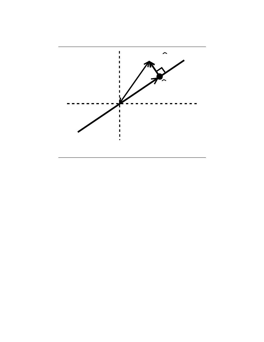
151
x
x-av
av
Figure 6.28:
7.13 Approximation and Projections in Hilbert Space
6.13.1 Introduction
Given a line ’l’ and a point ’p’ in the plane, what’s the closest point ’m’ to ’p’ on ’l’ ?
Same problem: Let x and v be vectors in R
2
. Say k v k= 1. For what value of α is
k x − αv k
2
minimized? (what point in span{v} best approximates x?)
The condition is that x − ˆ
αv and αv are orthogonal .
6.13.2 Calculating α
How to calculate ˆ
α?
We know that ( x − ˆ
αv) is perpendicular to every vector in span{v}, so
∀β, ∀β : x − ˆ
αv · βv = 0
β
∗
x · v − ˆ
αβ
∗
v · v = 0
because v · v = 1, so
x · v − ˆ
α = 0 ⇒ ˆ
α = x · v
Closest vector in span{v} = x · vv, where x · vv is the projection of x onto v.
Point to a plane?
We can do the same thing in higher dimensions.
Exercise 6.2:
Let V ⊂ H be a subspace of a Hilbert space H. Let x ∈ H be given. Find the
y ∈ V that best approximates x. i.e., k x − y k is minimized.

152
CHAPTER 6. HILBERT SPACES AND ORTHOGONAL EXPANSIONS
Figure 6.29:
Solution:
1.- Find an orthonormal basis (Section 6.7.3) {b
1
, . . . , b
k
} for V
2.- Project x onto V using
y =
k
X
i=1
(x · b
i
b
i
)
then y is the closest point in V to x and (x-y) ⊥ V ( ∀v, ∀v ∈ V : x − y · v = 0
Example 6.24:
x ∈ R
3
, V = span
1
0
0
,
0
1
0
, x =
a
b
c
. So,
y =
2
X
i=1
(x · b
i
b
i
) = a
1
0
0
+ b
0
1
0
=
a
b
0
Example 6.25:
V = {space of periodic signals with frequency no greater than 3w
0
}. Given periodic
f(t), what is the signal in V that best approximates f?
1.- {
1
√
T
e
jw
0
kt
, k = -3, -2, ..., 2, 3} is an ONB for V
2.- g (t) =
1
T
P
3
k=−3
f (t) · e
jw
0
kt
e
jw
0
kt
is the closest signal in V to f(t) ⇒
reconstruct f(t) using only 7 terms of its Fourier series.
Example 6.26:
Let V = {functions piecewise constant between the integers}
1.- ONB for V.
b
i
=
1 if i − 1 ≤ t < i
0 otherwise
where {b
i
} is an ONB.
Best piecewise constant approximation?
g (t) =
∞
X
i=−∞
(f · b
i
b
i
)
f · b
i
=
Z
∞
−∞
f (t) b
i
(t) dt =
Z
i
i−1
f (t) dt

Chapter 7
Fourier Analysis on Complex
Spaces
8.1 Fourier Analysis
Fourier analysis is fundamental to understanding the behavior of signals and systems. This is
a result of the fact that sinusoids are FIX ME - Eigenfunctions of linear, time-invariant (LTI)
systems. This is to say that if we pass any particular sinusoid through a LTI system, we get a
scaled version of that same sinusoid on the output. Then, since Fourier analysis allows us to
redefine the signals in terms of sinusoids, all we need to do is determine how any given system
effects all possible sinusoids (its transfer function) and we have a complete understanding
of the system. Furthermore, since we are able to define the passage of sinusoids through
a system as multiplication of that sinusoid by the transfer function at the same frequency,
we can convert the passage of any signal through a system from convolution (in time) to
multiplication (in frequency). These ideas are what give Fourier analysis its power.
Now, after hopefully having sold you on the value of this method of analysis, we must
examine exactly what we mean by Fourier analysis.
The four Fourier transforms that
comprise this analysis are the Fourier Series, Continuous-Time Fourier Transform, Discrete-
Time Fourier Transform and Discrete Fourier Transform. For this module, we will view
the Laplace Transform and Z-Transform as simply extensions of the CTFT and DTFT
respectively. All of these transforms act essentially the same way, by converting a signal
in time to an equivalent signal in frequency (sinusoids). However, depending on the nature
of a specific signal (ie whether it is finite- or infinite-length and whether it is discrete- or
continuous-time) there is an appropriate transform to convert the signal into the frequency
domain. Below is a table of the four Fourier transforms and when each is appropriate. It
also includes the relevant convolution for the specified space.
153

154
CHAPTER 7. FOURIER ANALYSIS ON COMPLEX SPACES
Table of Fourier Representations
Transform
Time Domain
Frequency Domain
Convolution
Continuous-Time
Fourier Series
L
2
([0, T ))
l
2
(Z)
Continuous-Time
Circular
Continuous-Time
Fourier Transform
L
2
(R)
L
2
(R)
Continuous-Time
Linear
Discrete-Time
Fourier Transform
l
2
(Z)
L
2
([0, 2π))
Discrete-Time
Lin-
ear
Discrete
Fourier
Transform
l
2
([0, N − 1])
l
2
([0, N − 1])
Discrete-Time
Cir-
cular
8.2 Fourier Analysis in Complex Spaces
7.2.1 Introduction
By now you should be familiar with the derivation of the Fourier series for continuous-time,
periodic functions. This derivation leads us to the following equations that you should be
quite familiar with:
f (t) =
X
n
c
n
e
jω
0
nt
(7.1)
c
n
=
1
T
R
n
f (t) e
−(jω
0
nt)
dt
=
1
T
f · e
jω
0
nt
(7.2)
where c
n
tells us the amount of frequency ω
0
n in f (t).
In this module, we will derive a similar expansion for discrete-time, periodic functions.
In doing so, we will derive the Discrete Time Fourier Series (DTFS), or the Discrete
Fourier Transform (DFT).
7.2.2 Derivation of DTFS
Much like a periodic, continuous-time function can be thought of as a function on the interval
[0, T ]
A periodic, discrete-time signal (with period N) can be thought of as a finite set of
numbers. For example, say we have the following set of numbers that describe a periodic,
discrete-time signal, where N = 4:
{. . . , 3, 2, −2, 1, 3, . . . }
We can represent this signal as either a periodic signal or as just a single interval as follows:
note:
The set of discrete time signals with period N equal C
N
.
Just like the continuous case, we are going to form a basis using harmonic sinusoids .
Before we look into this, it will be worth our time to look at the discrete-time, complex
sinusoids in a little more detail.
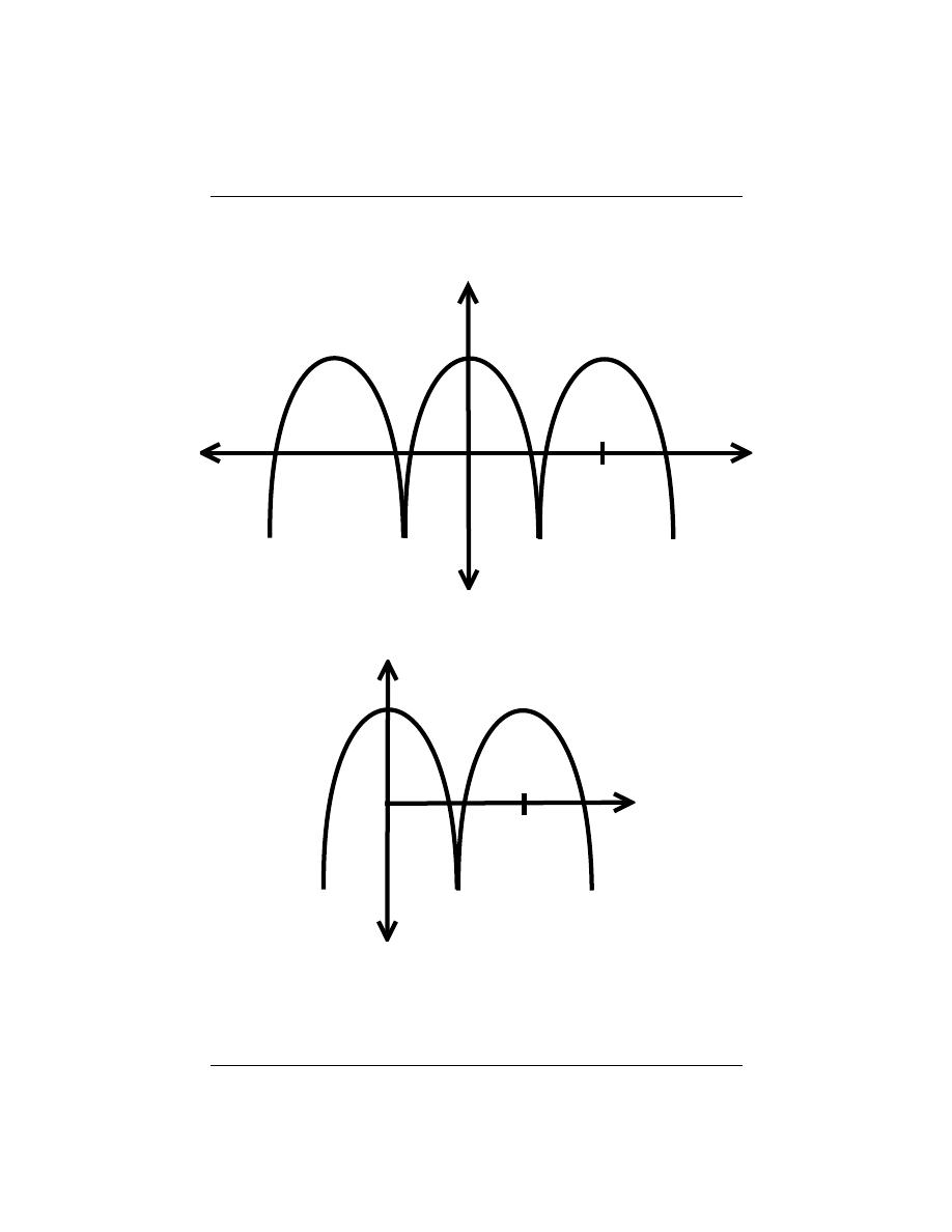
155
T
f(t)
(a)
T
(b)
Figure 7.1:
We will just consider one interval of the periodic function throughout this
section. (a) Periodic Function (b) Function on the interval [0, T ]
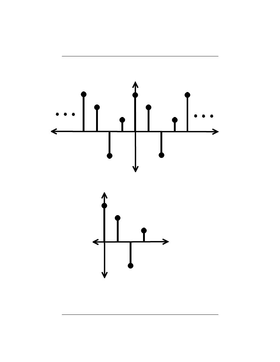
156
CHAPTER 7. FOURIER ANALYSIS ON COMPLEX SPACES
f[n]
n
(a)
n
(b)
Figure 7.2:
Here we can look at just one period of the signal that has a vector length
of four and is contained in C
4
. (a) Periodic Function (b) Function on the interval [0, T ]
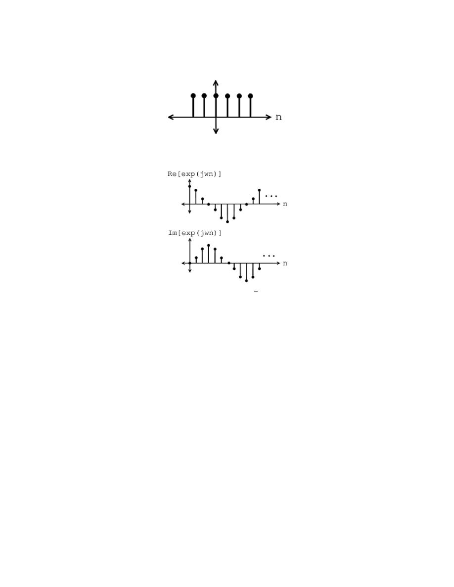
157
Figure 7.3:
Complex sinusoid with frequency ω = 0
Figure 7.4:
Complex sinusoid with frequency ω =
π
4
7.2.2.1 Complex Sinusoids
If you are familiar with the basic sinusoid signal and with complex exponentials then you
should not have any problem understanding this section. In most texts, you will see the the
discrete-time, complex sinusoid noted as:
e
jωn
Example 7.1:
Example 7.2:
7.2.2.1.1 In the Complex Plane
The complex sinusoid can be directly mapped onto our complex plane, which allows us to
easily visualize changes to the complex sinusoid and extract certain properties. The absolute
value of our complex sinusoid has the following characteristic:
∀n, n ∈ R : |e
jωn
| = 1
(7.3)
which tells that our complex sinusoid only takes values on the unit circle. As for the angle,
the following statement holds true:
∠e
jωn
= wn
(7.4)
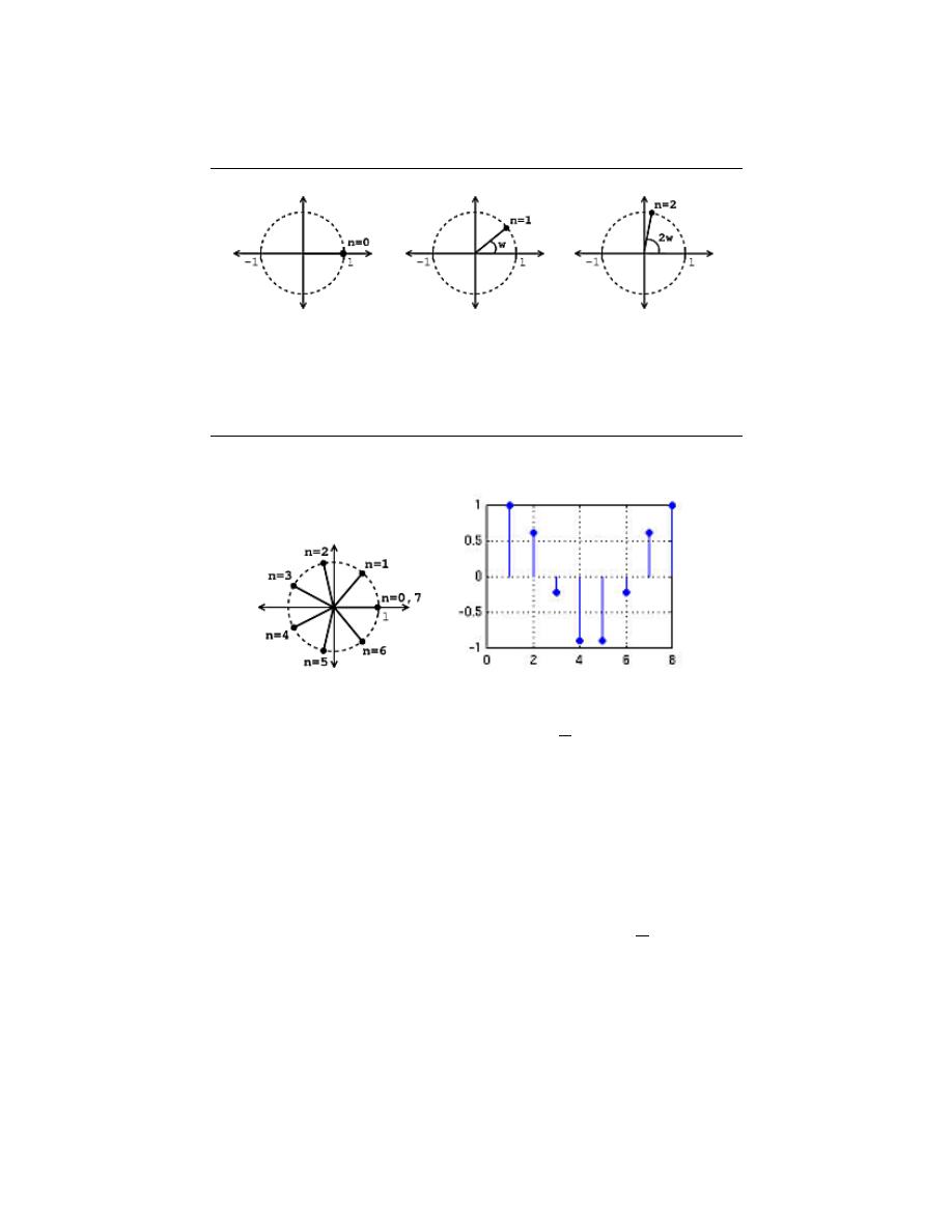
158
CHAPTER 7. FOURIER ANALYSIS ON COMPLEX SPACES
(a)
(b)
(c)
Figure 7.5:
These images show that as n increases, the value of e
jωn
moves around
the unit circle counterclockwise. (a) n = 0 (b) n = 1 (c) n = 2
(a)
(b)
Figure 7.6:
(a) N=7 (b) Here we have a plot of Re
e
j
2π
7
n
.
As n increases, we can picture e
jωn
equaling the values we get moving counterclockwise
around the unit circle. See the images below for an illustration:
note:
For e
jωn
to be periodic, we need e
jωN
= 1 for some N .
Example 7.3:
For our first example let us look at a periodic signal where ω =
2π
7
and N = 7.
Example 7.4:
Now let us look at the results of plotting a non-periodic siganl where ω = 1 and
N = 7.
7.2.2.1.2 Aliasing
Our complex sinusoids have the following property:
e
jωn
= e
j(ω+2π)n
(7.5)
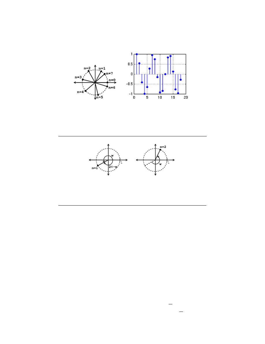
159
(a)
(b)
Figure 7.7:
(a) N=7 (b) Here we have a plot of Re e
jn
.
(a)
(b)
Figure 7.8:
Plot of our complex sinusoid with a frequency greater than pi.
Given this property, if we have a sinusoid with frequency ω + 2π, then this signal ”aliases”
to a sinusoid with frequency w.
note:
Each e
jωn
is unique for ω ∈ [0, 2π)
7.2.2.1.3 ”Negative” Frequencies
If we are given a signal with frequency π < ω < 2π, then this signal will be represented on
our complex plane as:
From the above images, the value of our complex sinusoid on the complex plane may
be more easily interpreted as cycling ”backwards” (clockwise) around the unit circle with
frequency 2π − ω. Rotating counterclockwise by w is the same as rotating clockwise by
2π − ω.
Example 7.5:
Let us plot our complex sinusoid, e
jωn
, where we have ω =
5π
4
and n = 1.
This plot is the same as a sinusoid with ”negative” frequency −
3π
4
.

160
CHAPTER 7. FOURIER ANALYSIS ON COMPLEX SPACES
Figure 7.9:
The above plot of our given frequency is identical to that of one where
ω = −
3π
4
.
point:
It makes more physical sense to chose [−π, π) as the interval for
ω.
Remember that e
jωn
and e
−(jωn)
are conjugates . This gives us the following notation
and property:
e
jωn∗
= e
−(jωn)
(7.6)
The real parts of of both exponentials in the above equation are the same; the imaginary
parts are negative of one another. This idea is the basic definition of a conjugate.
Now that we have looked over the concepts of complex sinusoids, let us turn our attention
back to finding a basis for discrete-time, periodic signals. After looking at all the complex
sinusoids, we must answer the question of which discrete-time sinusoids do we need to
represent periodic sequences with a perioid N .
Equivalent Question:
Find a set of vectors ∀n, n = {0, . . . , N − 1} : b
k
=
e
jω
k
n
such that {b
k
} are a basis for C
n
In answer to the above question, let us try the ”harmonic” sinusoids with a fundamental
frequency ω
0
=
2π
N
:
Harmonic Sinusoid
e
j
2π
N
kn
(7.7)
e
j
2π
N
kn
is periodic with period N and has k ”cycles” between n = 0 and n = N − 1.
Theorem 7.1:
If we let
∀n, n = {0, . . . , N − 1} : b
k
[n] =
1
√
N
e
j
2π
N
kn
where the exponential term is a vector in C
N
, then {b
k
} |
k={0,...,N −1}
is an or-
thonormal basis (Section 6.7.3) for C
N
.
Proof:
First of all, we must show {b
k
} is orthonormal, i.e. b
k
· b
l
= δ
kl
b
k
· b
l
=
N −1
X
n=0
b
k
[n] b
l
[n]
∗
=
1
N
N −1
X
n=0
e
j
2π
N
kn
e
−
(
j
2π
N
ln
)
b
k
· b
l
=
1
N
N −1
X
n=0
e
j
2π
N
(l−k)n
(7.8)
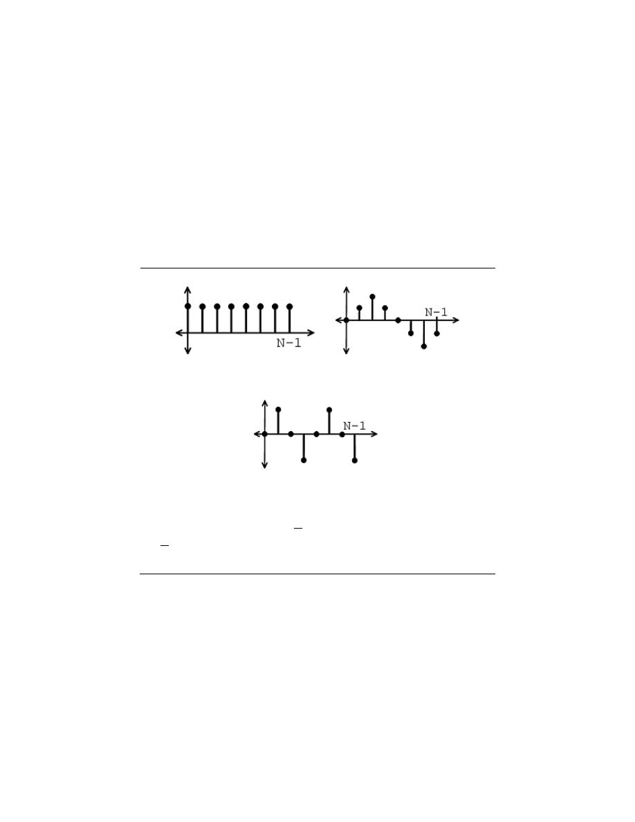
161
(a)
(b)
(c)
Figure 7.10:
Examples of our Harmonic Sinusoids (a) Harmonic sinusoid with k = 0
(b) Imaginary part of sinusoid, Im
e
j
2π
N
1n
, with k = 1 (c) Imaginary part of sinusoid,
Im
e
j
2π
N
2n
, with k = 2

162
CHAPTER 7. FOURIER ANALYSIS ON COMPLEX SPACES
If l = k, then
b
k
· b
l
=
1
N
P
N −1
n=0
(1)
=
1
(7.9)
If l 6= k, then we must use the ”partial summation formula” shown below:
N −1
X
n=0
(α
n
) =
∞
X
n=0
(α
n
) −
∞
X
n=N
(α
n
) =
1
1 − α
−
α
N
1 − α
=
1 − α
N
1 − α
b
k
· b
l
=
1
N
N −1
X
n=0
e
j
2π
N
(l−k)n
where in the above equation we can say that α = e
j
2π
N
(l−k)
, and thus we can see
how this is in the form needed to utilize our partial summation formula.
b
k
· b
l
=
1
N
1 − e
j
2π
N
(l−k)N
1 − e
j
2π
N
(l−k)
!
=
1
N
1 − 1
1 − e
j
2π
N
(l−k)
= 0
So,
b
k
· b
l
=
1 if k = l
0 if k 6= l
(7.10)
Therefore: {b
k
} is an orthonormal set. {b
k
} is also a basis (Section 4.1.3), since
there are N vectors which are linearly independent (Section 4.1.1) (orthoganality
implies linear independence).
And finally, we have shown that the harmonic sinusoids
n
1
√
N
e
j
2π
N
kn
o
form an
orthonormal basis for C
n
7.2.2.2 Discrete-Time Fourier Series (DTFS)
Using the steps shown above in the derivation and our previous understanding of Hilbert
Spaces and Orthogonal Expansions, the rest of the derivation is automatic. Given a discrete-
time, periodic signal (vector in C
n
) f [n], we can write:
f [n] =
1
√
N
N −1
X
k=0
c
k
e
j
2π
N
kn
(7.11)
c
k
=
1
√
N
N −1
X
n=0
f [n] e
−
(
j
2π
N
kn
)
(7.12)
Note: Most people collect both the
1
√
N
terms into the expression for c
k
.
Discrete Time Fourier Series:
Here is the common form of the DTFS with
the above note taken into account:
f [n] =
N −1
X
k=0
c
k
e
j
2π
N
kn
c
k
=
1
N
N −1
X
n=0
f [n] e
−
(
j
2π
N
kn
)
This what the fft command in MATLAB does.

163
8.3 Matrix Equation for the DTFS
The DTFS (Section 7.2.2.2) is just a change of basis (Section 4.1.3) in C
N
. To start, we
have f [n] in terms of the standard basis.
f [n]
=
f [0] e
0
+ f [1] e
1
+ · · · + f [N − 1] e
N −1
=
P
n−1
k=0
(f [k] δ [k − n])
(7.13)
f [0]
f [1]
f [2]
..
.
f [N − 1]
=
f [0]
0
0
..
.
0
+
0
f [1]
0
..
.
0
+
0
0
f [2]
..
.
0
+ · · · +
0
0
0
..
.
f [N − 1]
(7.14)
Taking the DTFS, we can write f [n] in terms of the sinusoidal Fourier basis
f [n] =
N −1
X
k=0
c
k
e
j
2π
N
kn
(7.15)
f [0]
f [1]
f [2]
..
.
f [N − 1]
= c
0
1
1
1
..
.
1
+ c
1
1
e
j
2π
N
e
j
4π
N
..
.
e
j
2π
N
(N −1)
+ c
2
1
e
j
4π
N
e
j
8π
N
..
.
e
j
4π
N
(N −1)
+ . . .
(7.16)
We can form the basis matrix (we’ll call it W here instead of B) by stacking the basis vectors
in as columns
W
=
b
0
[n]
b
1
[n]
. . .
b
N −1
[n]
=
1
1
1
. . .
1
1
e
j
2π
N
e
j
4π
N
. . .
e
j
2π
N
(N −1)
1
e
j
4π
N
e
j
8π
N
. . .
e
j
2π
N
2(N −1)
..
.
..
.
..
.
..
.
..
.
1
e
j
2π
N
(N −1)
e
j
2π
N
2(N −1)
. . .
e
j
2π
N
(N −1)(N −1)
(7.17)
with b
k
[n] = e
j
2π
N
kn
note:
the entry in the k-th row and n-th column is W
j,k
= e
j
2π
N
kn
= W
n,k
So, here we have an additional symmetry
W = W
T
⇒ W
T ∗
= W
∗
=
1
N
W
−1
(since {b
k
[n]} are orthogonal)
We can now rewrite the DTFS equations in matrix form where we have:
• - f = signal (vector in C
N
)
• - c = DTFS coeffs. (vector in C
N
)

164
CHAPTER 7. FOURIER ANALYSIS ON COMPLEX SPACES
”synthesis”
f = W c
f [n] = c · b
n
∗
”analysis”
c = W
T ∗
f = W
∗
f
c [k] = f · b
k
Finding (and inverting) the DTFS is just matrix multiplication.
Everything in C
N
is clean: no limits, no convergence questions, just good ole matrix
arithmetic.
8.4 Periodic Extension to DTFS
7.4.1 Introduction
Now that we have an understanding of the discrete-time Fourier series (DTFS) (Section 7.2.2.2),
we can consider the periodic extension of c [k] (the Discrete-time Fourier coefficients). The
basic figures below show a simple illustration of how we can represent a sequence as a
periodic signal mapped over an infinite number of intervals.
Exercise 7.1:
Why does a periodic extension to the DTFS coefficients c [k] make sense?
Solution:
Aliasing: b
k
= e
j
2π
N
kn
b
k+N
=
e
j
2π
N
(k+N )n
=
e
j
2π
N
kn
e
j2πn
=
e
j
2π
N
n
=
b
k
(7.18)
→ DTFS coefficients are also periodic with period N.
7.4.2 Examples
Example 7.6:
Discrete time square wave
Calculate the DTFS c [k] using:
c [k] =
1
N
N −1
X
n=0
f [n] e
−
(
j
2π
N
kn
)
(7.19)
Just like continuous time Fourier series, we can take the summation over any
interval, so we have
c
k
=
1
N
N
1
X
n=−N
1
e
−
(
j
2π
N
kn
)
(7.20)
Let m = n + N
1
(so we can get a geometric series starting at 0)
c
k
=
1
N
P
2N
1
m=0
e
−
(
j
2π
N
(m−N
1
)k
)
=
1
N
e
j
2π
N
k
P
2N
1
m=0
e
−
(
j
2π
N
mk
)
(7.21)
Now, using the ”partial summation formula”
M
X
n=0
(a
n
) =
1 − a
M +1
1 − a
(7.22)

165
(a)
(b)
Figure 7.11:
(a) vectors (b) periodic sequences
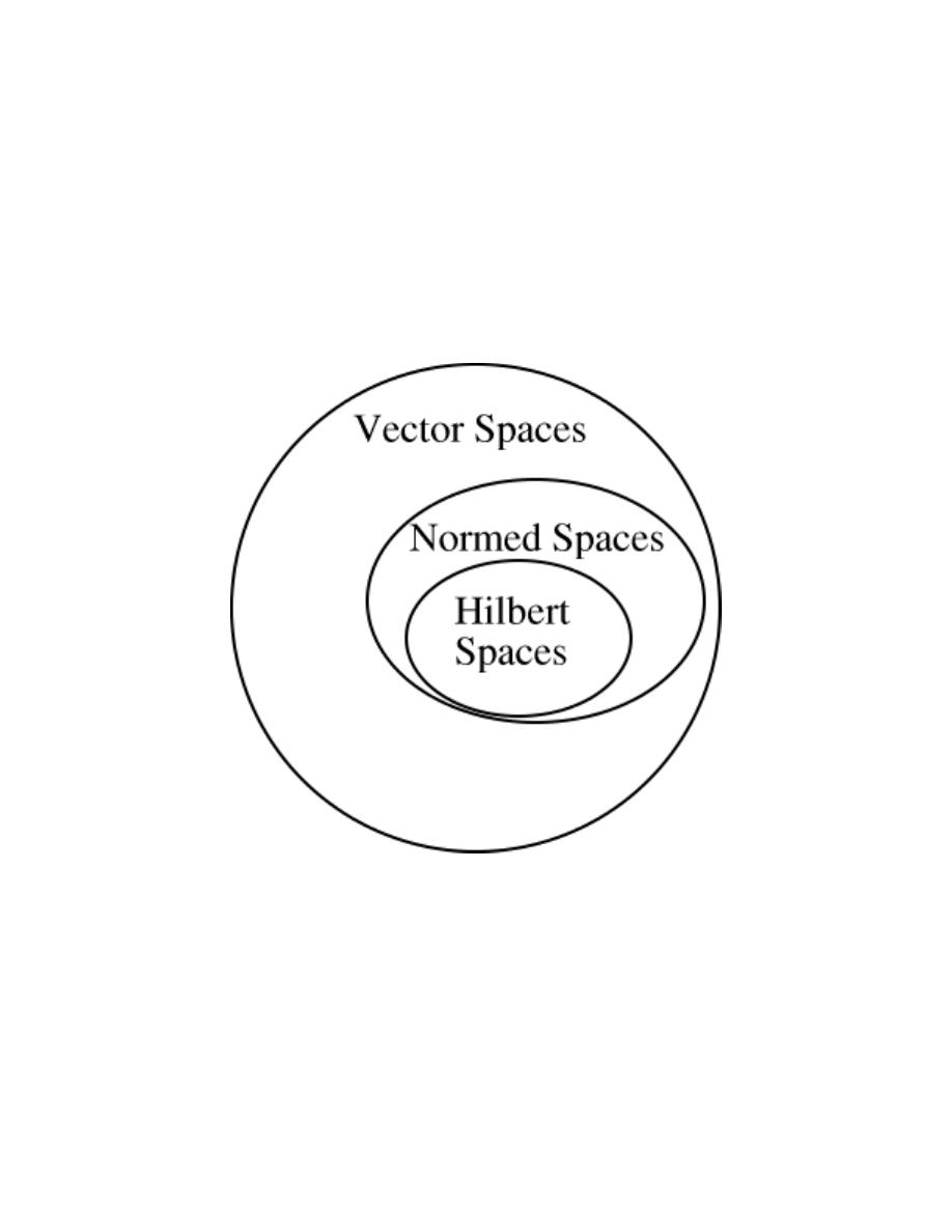
166
CHAPTER 7. FOURIER ANALYSIS ON COMPLEX SPACES
Figure 7.12
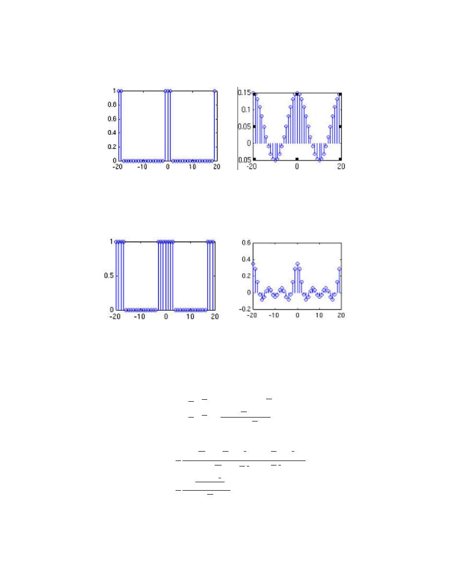
167
(a)
(b)
Figure 7.13:
N
1
= 1 (a) Plot of f [n]. (b) Plot of c [k].
(a)
(b)
Figure 7.14:
N
1
= 3 (a) Plot of f [n]. (b) Plot of c [k].
c
k
=
1
N
e
j
2π
N
N
1
k
P
2N
1
m=0
e
−
(
j
2π
N
k
)
m
=
1
N
e
j
2π
N
N
1
k 1−e
−
(
j 2π
N
(2N1+1)
)
1−e
−
(
jk 2π
N
)
(7.23)
Manipulate to make this look this sinc (distribute)
c
k
=
1
N
e
−
(
jk 2π
2N
)
e
jk 2π
N
(
N1+
1
2
)
−e
−
(
jk 2π
N
(
N1+
1
2
))
e
−
(
jk 2π
2N
)
e
jk 2π
N
1
2
−e
−
(
jk 2π
N
1
2
)
=
1
N
sin
2πk
(
N1+
1
2
)
N
!
sin
(
πk
N
)
=
digital sinc
(7.24)
note:
It’s periodic! The illustration below show our above function and
coefficients for various values of N
1
.
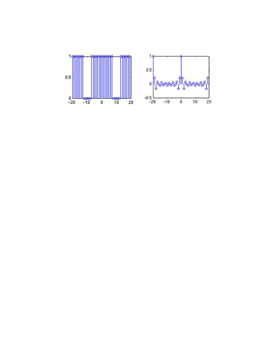
168
CHAPTER 7. FOURIER ANALYSIS ON COMPLEX SPACES
(a)
(b)
Figure 7.15:
N
1
= 7 (a) Plot of f [n]. (b) Plot of c [k].
Example 7.7:
Bird song
Example 7.8:
DFT Spectral Analysis
Example 7.9:
Signal Recovery
Example 7.10:
Compression (1-D)
Example 7.11:
Image Compression
8.5 Circular Shifts
The many properties of the DFT (Section 7.2.2.2) become really straightforward ( very
similar to the Fourier Series) once we have once concept down: Circular Shifts .
7.5.1 Circular shifts
We can picture periodic sequences as having discrete points on a circle as the domain
Shifting by m, f (n + m), corresponds to rotating the cylinder m notches ACW (counter
clockwise). For m = −2, we get a shift equal to that in the following illustration:
To cyclic shift we follow these steps:
1) Write f (n) on a cylinder, ACW
2) To cyclic shift by m, spin cylinder m spots ACW
f [n] → f [((n + m))
N
]
Example 7.12:
If f (n) = [0, 1, 2, 3, 4, 5, 6, 7], then f (((n − 3))
N
) = [3, 4, 5, 6, 7, 0, 1, 2]
It’s called circular shifting , since we’re moving around the circle. The usual
shifting is called ”linear shifting” (shifting along a line).

169
Figure 7.16

170
CHAPTER 7. FOURIER ANALYSIS ON COMPLEX SPACES
Figure 7.17

171
Figure 7.18

172
CHAPTER 7. FOURIER ANALYSIS ON COMPLEX SPACES
Figure 7.19

173
(a)
(b)
Figure 7.20: We’ve cut down on storage space by >90% (while incurring some loss) (a)
256 by 256 image (65,636 pixels) (b) Reconstructed using only 6000 coefficients
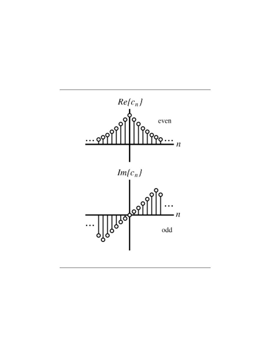
174
CHAPTER 7. FOURIER ANALYSIS ON COMPLEX SPACES
Figure 7.21
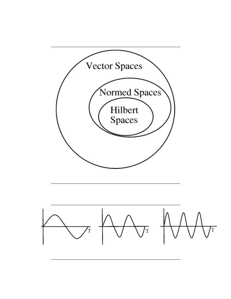
175
Figure 7.22: for m = −2
Figure 7.23
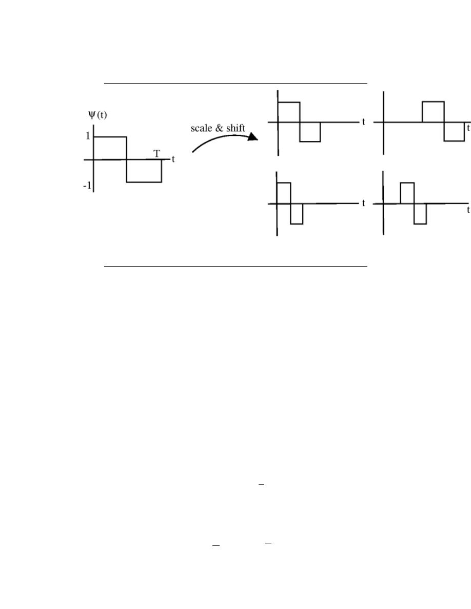
176
CHAPTER 7. FOURIER ANALYSIS ON COMPLEX SPACES
Figure 7.24: N=8
7.5.1.1 Notes on circular shifting
f [((n + N ))
N
] = f [n]
Spinning N spots is the same as spinning all the way around, or not spinning at all.
f [((n + N ))
N
] = f [((n − (N − m)))
N
]
Shifting ACW m is equivalent to shifting CW N − m
f [((−n))
N
]
The above expression, simply writes the values of f [n] clockwise.
7.5.2 Circular shifts and the DFT
Theorem 7.2:
Circular Shifts and DFT
If
f [n]
DFT
↔ F [k]
then
f [((n − m))
N
]
DFT
↔ e
−
(
j
2π
N
km
)F [k]
(i.e. circular shift in time domain = phase shift in DFT)
Proof:
f [n] =
1
N
N −1
X
k=0
F [k] e
j
2π
N
kn
(7.25)

177
Figure 7.25: m=-3
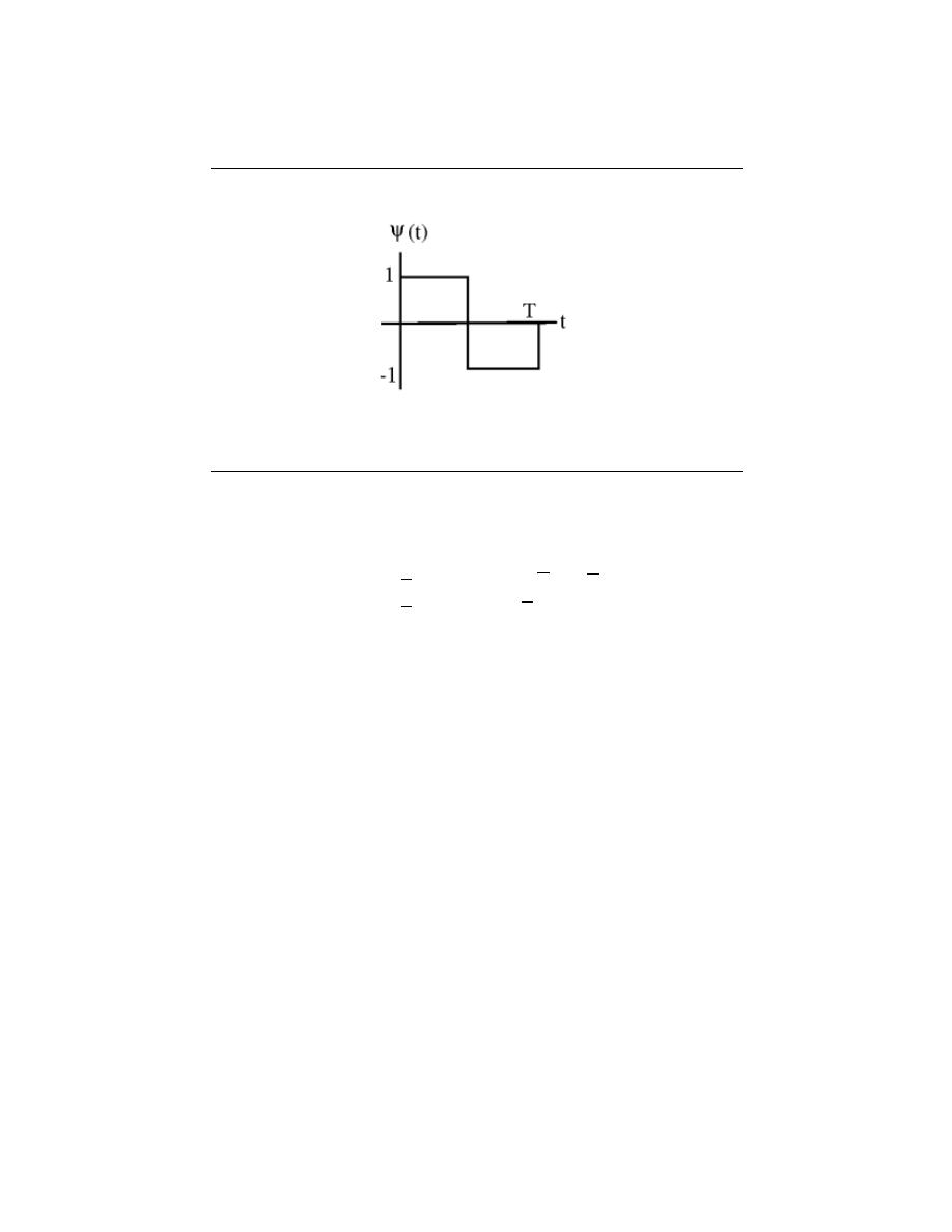
178
CHAPTER 7. FOURIER ANALYSIS ON COMPLEX SPACES
Figure 7.26
so phase shifting the DFT
f [n]
=
1
N
P
N −1
k=0
F [k] e
−
(
j
2π
N
kn
)e
j
2π
N
kn
=
1
N
P
N −1
k=0
F [k] e
j
2π
N
k(n−m)
=
f [((n − m))
N
]
(7.26)
8.6 Circular Convolution and the DFT
7.6.1 Introduction
You should be familiar with Discrete-Time Convolution, which tells us that given two
discrete-time signals x [n], the system’s input, and h [n], the system’s response, we define
the output of the system as
y [n]
=
x [n] ∗ h [n]
=
P
∞
k=−∞
(x [k] h [n − k])
(7.27)
When we are given two DFTs (finite-length sequences usually of length N ), we cannot just
multiply them together as we do in the above convolution formula, often referred to as linear
convolution . Because the DFTs are periodic, they have nonzero values for n ≥ N and thus
the multiplication of these two DFTs will be nonzero for n ≥ N . We need to define a new
type of convolution operation that will result in our convolved signal being zero outside of
the range n = {0, 1, . . . , N − 1}. This idea led to the development of circular convolution
, also called cyclic or periodic convolution.
7.6.2 Circular Convolution Formula
What happens when we multiply two DFT’s together, where Y [k] is the DFT of y [n]?
Y [k] = F [k] H [k]
(7.28)
when 0 ≤ k ≤ N − 1
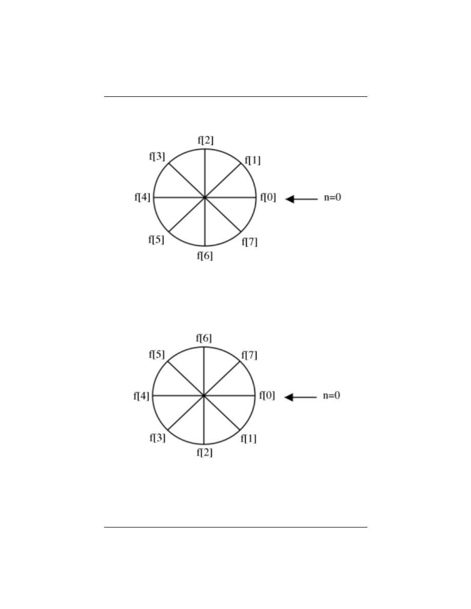
179
(a)
(b)
Figure 7.27:
(a) f [n] (b) f
((−n))
N
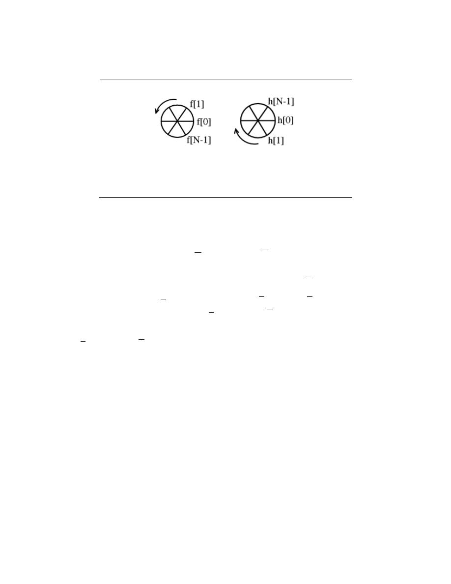
180
CHAPTER 7. FOURIER ANALYSIS ON COMPLEX SPACES
(a)
(b)
Figure 7.28:
Step 1
Using the DFT synthesis formula for y [n]
y [n] =
1
N
N −1
X
k=0
F [k] H [k] e
j
2π
N
kn
(7.29)
And then applying the analysis formula F [k] =
P
N −1
m=0
f [m] e
(−j)
2π
N
kn
y [n]
=
1
N
P
N −1
k=0
P
N −1
m=0
f [m] e
(−j)
2π
N
kn
H [k] e
j
2π
N
kn
=
P
N −1
m=0
f [m]
1
N
P
N −1
k=0
H [k] e
j
2π
N
k(n−m)
(7.30)
where we can reduce the second summation found in the above equation into h [((n − m))
N
] =
1
N
P
N −1
k=0
H [k] e
j
2π
N
k(n−m)
y [n] =
N −1
X
m=0
(f [m] h [((n − m))
N
])
which equals circular convolution! When we have 0 ≤ n ≤ N − 1 in the above, then we get:
y [n] ≡ (f [n] @@h [n])
(7.31)
note:
The notation @@ represents cyclic convolution ”mod N”.
7.6.2.1 Steps for Cyclic Convolution
Steps for cyclic convolution are the same as the usual convo, except all index calculations
are done ”mod N” = ”on the wheel”
Steps for Cyclic Convolution
• - Step 1: ”Plot” f [m] and h [((−m))
N
]
• - Step 2: ”Spin” h [((−m))
N
] n notches ACW (counter-clockwise) to get h [((n − m))
N
]
(i.e. Simply rotate the sequence, h [n], clockwise by n steps).
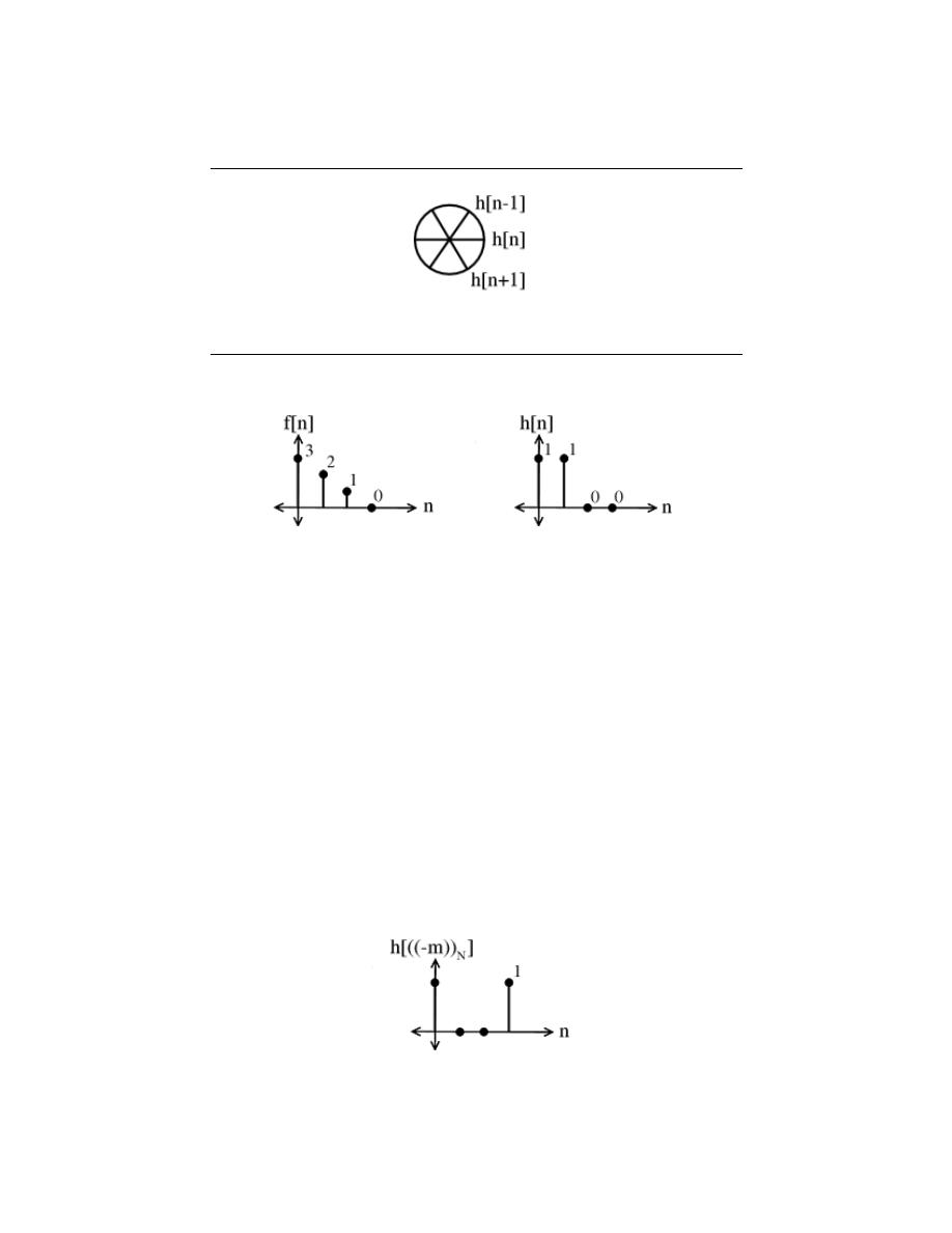
181
Figure 7.29:
Step 2
(a)
(b)
Figure 7.30:
Two discrete-time signals to be convolved.
• - Step 3: Pointwise multiply the f [m] wheel and the h [((n − m))
N
] wheel.
sum = y [n]
• - Step 4: Repeat for all 0 ≤ n ≤ N − 1
Example 7.13:
Convolve (n = 4)
•- h [((−m))
N
]
Multiply f [m] and sum to yield: y [0] = 3
•- h [((1 − m))
N
]
Figure 7.31
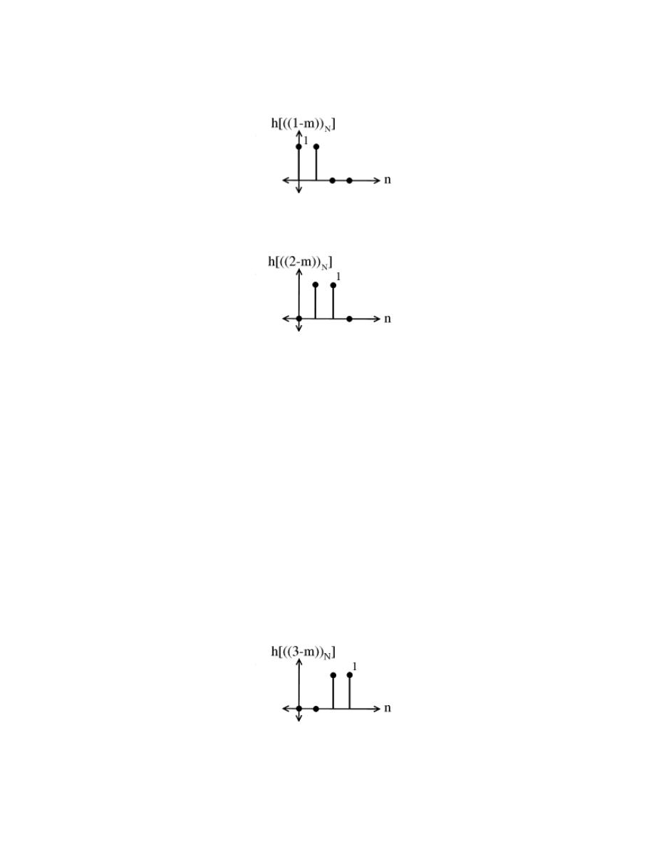
182
CHAPTER 7. FOURIER ANALYSIS ON COMPLEX SPACES
Figure 7.32
Figure 7.33
Multiply f [m] and sum to yield: y [1] = 5
•- h [((2 − m))
N
]
Multiply f [m] and sum to yield: y [2] = 3
•- h [((3 − m))
N
]
Multiply f [m] and sum to yield: y [3] = 1
7.6.2.2 Alternative Algorithm
Alternative Circular Convolution Algorithm
• - Step 1: Calculate the DFT of f [n] which yields F [k] and calculate the DFT of h [n]
which yields H [k].
• - Step 2: Pointwise multiply Y [k] = F [k] H [k]
Figure 7.34

183
• - Step 3: Inverse DFT Y [k] which yields y [n]
Seems like a roundabout way of doing things, but it turns out that there are extremely
fast ways to calculate the DFT of a sequence.
To circularily convolve 2 N -point sequences:
y [n] =
N −1
X
m=0
(f [m] h [((n − m))
N
])
For each n : N multiples, N − 1 additions
N points implies N
2
multiplications, N (N − 1) additions implies O N
2
complexity.
8.7 DFT: Fast Fourier Transform
We now have a way of computing the spectrum for an arbitrary signal: The Discrete Fourier
Transform (DFT) (pg ??) computes the spectrum at N equally spaced frequencies from a
length- N sequence. An issue that never arises in analog ”computation,” like that performed
by a circuit, is how much work it takes to perform the signal processing operation such as
filtering. In computation, this consideration translates to the number of basic computa-
tional steps required to perform the needed processing. The number of steps, known as the
complexity , becomes equivalent to how long the computation takes (how long must we
wait for an answer). Complexity is not so much tied to specific computers or programming
languages but to how many steps are required on any computer. Thus, a procedure’s stated
complexity says that the time taken will be proportional to some function of the amount
of data used in the computation and the amount demanded.
For example, consider the formula for the discrete Fourier transform. For each frequency
we chose, we must multiply each signal value by a complex number and add together the
results. For a real-valued signal, each real-times-complex multiplication requires two real
multiplications, meaning we have 2N multiplications to perform. To add the results to-
gether, we must keep the real and imaginary parts separate. Adding N numbers requires
N − 1 additions. Consequently, each frequency requires 2N + 2 (N − 1) = 4N − 2 ba-
sic computational steps. As we have N frequencies, the total number of computations is
N (4N − 2).
In complexity calculations, we only worry about what happens as the data lengths in-
crease, and take the dominant term–here the 4N
2
term–as reflecting how much work is
involved in making the computation. As multiplicative constants don’t matter since we
are making a ”proportional to” evaluation, we find the DFT is an O N
2
computational
procedure. This notation is read ”order N -squared”. Thus, if we double the length of the
data, we would expect that the computation time to approximately quadruple.
Exercise 7.2:
In making the complexity evaluation for the DFT, we assumed the data to be real.
Three questions emerge. First of all, the spectra of such signals have conjugate
symmetry, meaning that negative frequency components (k =
N
2
+ 1, ..., N + 1
in the DFT (pg ??)) can be computed from the corresponding positive frequency
components. Does this symmetry change the DFT’s complexity?
Secondly, suppose the data are complex-valued; what is the DFT’s complexity
now?
Finally, a less important but interesting question is suppose we want K frequency
values instead of N ; now what is the complexity?
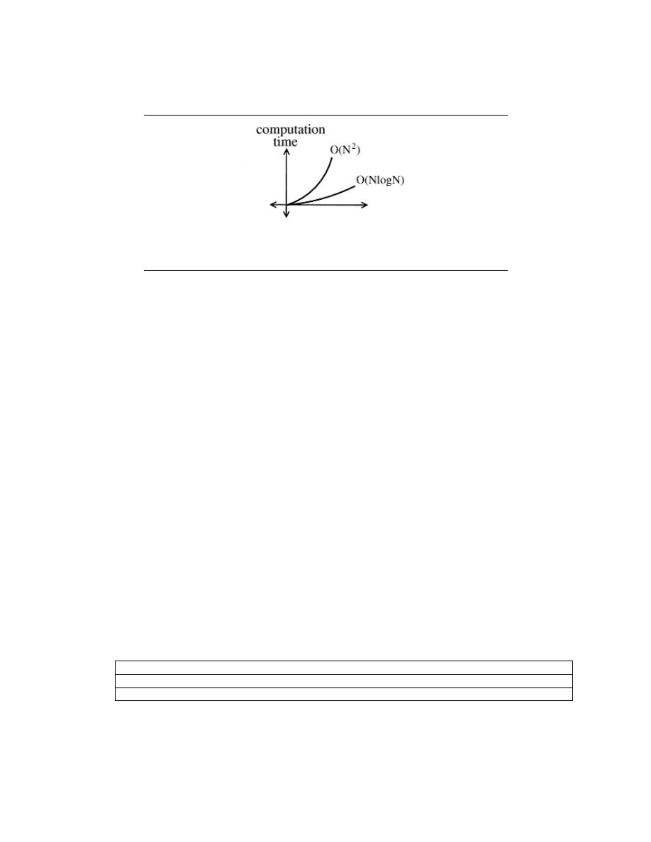
184
CHAPTER 7. FOURIER ANALYSIS ON COMPLEX SPACES
Figure 7.35:
The figure above shows how much slower the computation time of an
O(NlogN) process grows.
Solution:
When the signal is real-valued, we may only need half the spectral values, but the
complexity remains unchanged. If the data are complex-valued, which demands
retaining all frequency values, the complexity is again the same. When only K
frequencies are needed, the complexity is O (KN).
8.8 The Fast Fourier Transform (FFT)
7.8.1 Introduction
The Fast Fourier Transform (FFT) is an efficient O(NlogN) algorithm for calculating DFTs
• - originally discovered by Gauss in the early 1800’s
• - rediscovered by Cooley and Tukey at IBM in the 1960’s
• - C.S. Burrus, Rice University’s very own Dean of Engineering, literally ”wrote the
book” on fast DFT algorithms.
The FFT exploits symmetries in the W matrix to take a ”divide and conquer” approach.
We won’t talk about the actual FFT algorithm here, see these notes if you are interested in
reading a little more on the idea behind FFT.
7.8.2 Speed Comparison
How much better is O(NlogN) than O( N
2
)?
N
10
100
1000
10
6
10
9
N
2
100
10
4
10
6
10
12
10
18
N logN
1
200
3000
6 × 10
6
9 × 10
9
Say you have a 1 MFLOP machine (a million ”floating point” operations per second).
Let N = 1 million = 10
6
.
An O( N
2
) algorithm takes 10
12
flors → 10
6
seconds @@@ 11.5 days.
An O( N logN ) algorithm takes 6 × 10
6
Flors → 6 seconds.

185
note:
N = 1 million is not unreasonable.
Example 7.14:
3 megapixel digital camera spits out 3 × 10
6
numbers for each picture. So for two
N point sequences f [n] and h [n]. If computing (f [n] @@h [n]) directly: O( N
2
)
operations.
taking FFTs – O(NlogN)
multiplying FFTs – O(N)
inverse FFTs – O(NlogN).
the total complexity is O(NlogN).
note:
FFT + digital computer were almost completely responsible for
the ”explosion” of DSP in the 60’s.
note:
Rice was (and still is) one of the places to do research in DSP.
8.9 Deriving the Fast Fourier Transform
To derive the FFT, we assume that the signal’s duration is a power of two: N = 2
l
.
Consider what happens to the even-numbered and odd-numbered elements of the sequence
in the DFT calculation.
S (k)
=
s (0) + s (2) e
(−j)
2π2k
N
+ · · · + s (N − 2) e
(−j)
2π(N −2)k
N
+ s (1) e
(−j)
2πk
N
+ s (3) e
(−j)
2π(2+1)k
N
+ · · · + s (N − 1) e
(−j)
2π(N −2+1)k
N
=
s (0) + s (2) e
(−j)
2πk
N
2
+ · · · + s (N − 2) e
(−j)
2π
(
N
2
−1
)
k
N
2
+
s (1) + s (3) e
(−j)
2πk
N
2
+ · · · + s (N − 1) e
(−j)
2π
(
N
2
−1
)
k
N
2
e
−(j2πk)
N
(7.32)
Each term in square brackets has the form of a
N
2
-length DFT. The first one is a
DFT of the even-numbered elements, and the second of the odd-numbered elements. The
first DFT is combined with the second multiplied by the complex exponential e
−(j2πk)
N
.
The half-length transforms are each evaluated at frequency indices k ∈ {0, . . . , N − 1} .
Normally, the number of frequency indices in a DFT calculation range between zero and
the transform length minus one. The computational advantage of the FFT comes from
recognizing the periodic nature of the discrete Fourier transform. The FFT simply reuses
the computations made in the half-length transforms and combines them through additions
and the multiplication by e
−(j2πk)
N
, which is not periodic over
N
2
, to rewrite the length-N
DFT. Figure 7.36 illustrates this decomposition. As it stands, we now compute two length-
N
2
transforms (complexity 2O
N
2
4
), multiply one of them by the complex exponential
(complexity O (N ) ), and add the results (complexity O (N ) ). At this point, the total
complexity is still dominated by the half-length DFT calculations, but the proportionality
coefficient has been reduced.
Now for the fun. Because N = 2
l
, each of the half-length transforms can be reduced to
two quarter-length transforms, each of these to two eighth-length ones, etc. This decompo-
sition continues until we are left with length-2 transforms. This transform is quite simple,
involving only additions. Thus, the first stage of the FFT has
N
2
length-2 transforms (see
the bottom part of Figure 7.36). Pairs of these transforms are combined by adding one
to the other multiplied by a complex exponential. Each pair requires 4 additions and 4

186
CHAPTER 7. FOURIER ANALYSIS ON COMPLEX SPACES
multiplications, giving a total number of computations equaling 8
N
4
=
N
2
. This number
of computations does not change from stage to stage. Because the number of stages, the
number of times the length can be divided by two, equals log
2
N , the complexity of the
FFT is O (N logN ) .
Doing an example will make computational savings more obvious. Let’s look at the
details of a length-8 DFT. As shown on Figure 7.36, we first decompose the DFT into
two length-4 DFTs, with the outputs added and subtracted together in pairs. Considering
Figure 7.36 as the frequency index goes from 0 through 7, we recycle values from the length-
4 DFTs into the final calculation because of the periodicity of the DFT output. Examining
how pairs of outputs are collected together, we create the basic computational element
known as a butterfly (Figure 7.37).
By considering together the computations involving common output frequencies from the
two half-length DFTs, we see that the two complex multiplies are related to each other, and
we can reduce our computational work even further. By further decomposing the length-4
DFTs into two length-2 DFTs and combining their outputs, we arrive at the diagram sum-
marizing the length-8 fast Fourier transform (Figure 7.36). Although most of the complex
multiplies are quite simple (multiplying by e
−(jπ)
means negating real and imaginary parts),
let’s count those for purposes of evaluating the complexity as full complex multiplies. We
have
N
2
= 4 complex multiplies and 2N = 16 additions for each stage and log
2
N = 3 stages,
making the number of basic computations
3N
2
log
2
N as predicted.
Exercise 7.3:
Note that the ordering of the input sequence in the two parts of Figure 7.36 aren’t
quite the same. Why not? How is the ordering determined?
Solution:
The upper panel has not used the FFT algorithm to compute the length-4 DFTs
while the lower one has. The ordering is determined by the algorithm.
Other ”fast” algorithms were discovered, all of which make use of how many common
factors the transform length N has. In number theory, the number of prime factors a given
integer has measures how composite it is. The numbers 16 and 81 are highly composite
(equaling 2
4
and 3
4
respectively), the number 18 is less so ( 2
1
3
2
), and 17 not at all
(it’s prime). In over thirty years of Fourier transform algorithm development, the original
Cooley-Tukey algorithm is far and away the most frequently used. It is so computationally
efficient that power-of-two transform lengths are frequently used regardless of what the
actual length of the data.
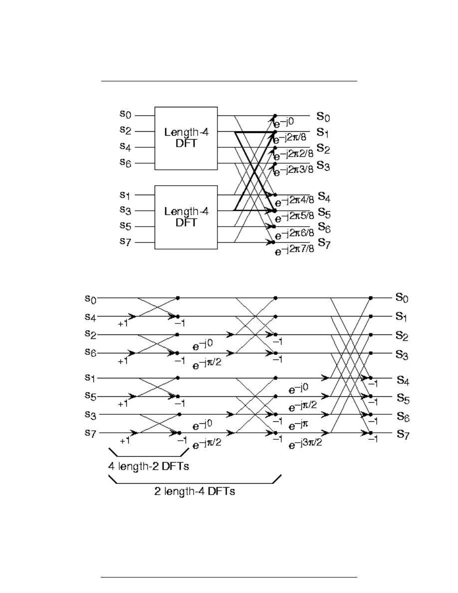
187
Length-8 DFT decomposition
(a)
(b)
Figure 7.36:
The initial decomposition of a length-8 DFT into the terms using even-
and odd-indexed inputs marks the first phase of developing the FFT algorithm. When
these half-length transforms are successively decomposed, we are left with the diagram
shown in the bottom panel that depicts the length-8 FFT computation.
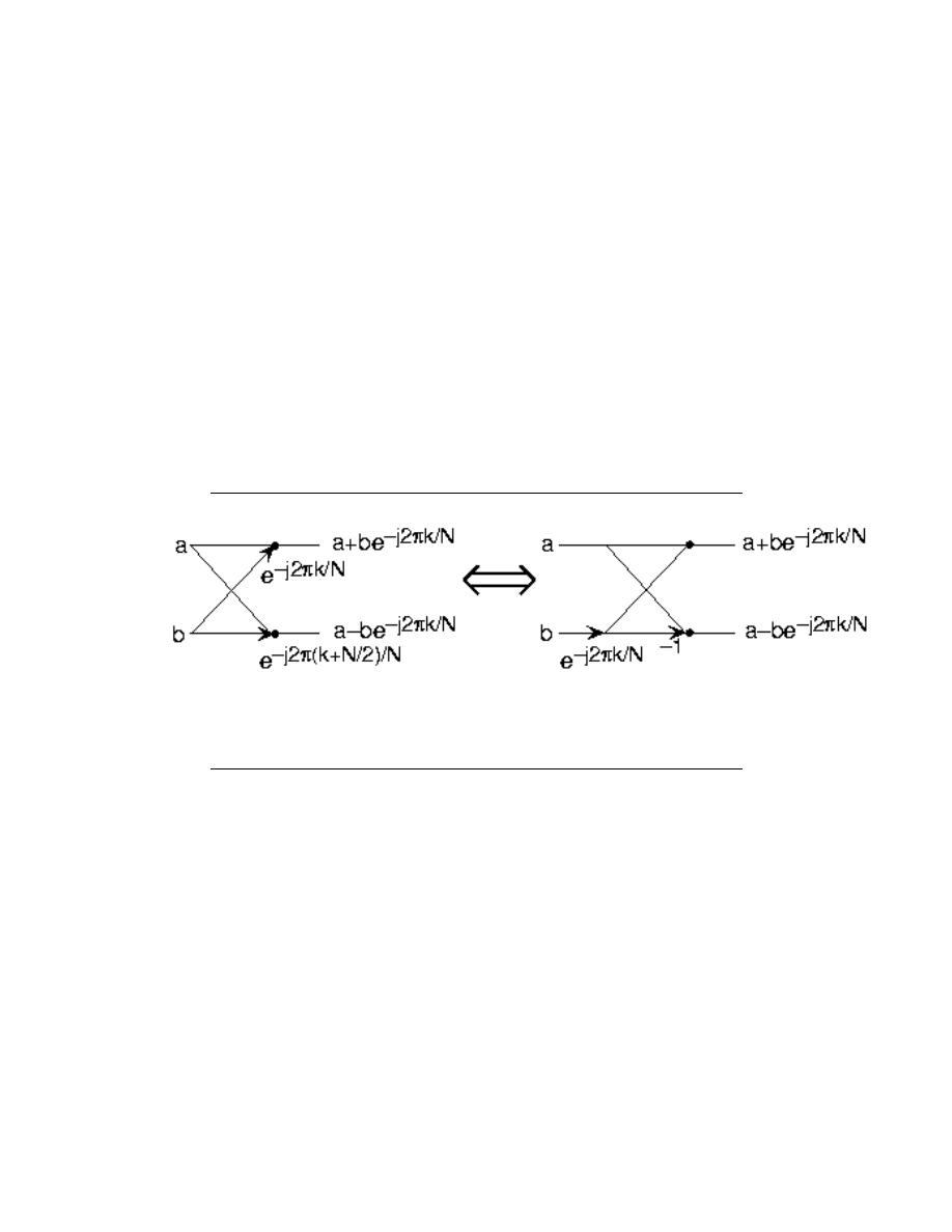
188
CHAPTER 7. FOURIER ANALYSIS ON COMPLEX SPACES
Butterfly
Figure 7.37:
The basic computational element of the fast Fourier transform is the
butterfly. It takes two complex numbers, represented by a and b, and forms the quantities
shown. Each butterfly requires one complex multiplication and two complex additions.

Chapter 8
Convergence
9.1 Convergence of Sequences
8.1.1 What is a Sequence?
sequence :
A sequence is a function g
n
defined on the positive intergers ’n’. We
often denote a sequence by {g
n
} |
∞
n=1
Example 61:
A real number sequence:
g
n
=
1
n
Example 62:
A vector sequence:
g
n
=
sin
nπ
2
cos
nπ
2
Example 63:
A function sequence:
g
n
(t) =
1 if 0 ≤ t <
1
n
0 otherwise
note:
A function can be thought of as an infinite dimensional
vector where for each value of ’t’ we have one dimension
8.1.2 Convergence of Real Sequences
limit :
A sequence {g
n
} |
∞
n=1
converges to a limit g ∈ R if for every > 0 there
is an integer N such that
∀i, i ≥ N : |g
i
− g| <
We usually denote a limit by writing
lim
i→∞
g
i
= g
or
g
i
→ g
189

190
CHAPTER 8. CONVERGENCE
The above definition means that no matter how small we make , except for a finite number
of g
i
’s, all points of the sequence are within distance of g.
Example 8.1:
We are given the following convergent sequence:
g
n
=
1
n
(8.1)
Intuitively we can assume the following limit:
lim
n→∞
g
n
= 0
Let us prove this rigorously. Say that we are given a real number > 0. Let us
choose N = d
1
e, where dxe denotes the smallest integer larger than x. Then for
n ≥ N we have
|g
n
− 0| =
1
n
≤
1
N
<
Thus,
lim
n→∞
g
n
= 0
Example 8.2:
Now let us look at the following non-convergent sequence
g
n
=
1 if n = even
−1 if n = odd
This sequence oscillates between 1 and -1, so it will therefore never converge.
8.1.2.1 Problems
For practice, say which of the following sequences converge and give their limits if they exist.
1. - g
n
= n
2. - g
n
=
1
n
if n = even
−1
n
if n = odd
3. - g
n
=
1
n
if n 6= powerof10
1 otherwise
4. - g
n
=
n if n < 10
5
1
n
if n ≥ 10
5
5. - g
n
= sin
π
n
6. - g
n
= j
n
9.2 Convergence of Vectors
8.2.1 Convergence of Vectors
We now discuss pointwise and norm convergence of vectors. Other types of convergence also
exist, and one in particular, uniform convergence, can also be studied. For this discussion ,
we will assume that the vectors belong to a normed vector space.

191
8.2.1.1 Pointwise Convergence
A sequence {g
n
} |
∞
n=1
converges pointwise to the limit g if each element of g
n
converges to
the corresponding element in g. Below are few examples to try and help illustrate this idea.
Example 8.3:
g
n
=
g
n
[1]
g
n
[2]
=
1 +
1
n
2 −
1
n
First we find the following limits for our two g
n
’s:
lim
n→∞
(g
n
[1]) = 1
lim
n→∞
(g
n
[2]) = 2
Therefore we have the following,
lim
n→∞
g
n
= g
pointwise, where g =
1
2
.
Example 8.4:
∀t, t ∈ R : g
n
(t) =
t
n
As done above, we first want to examine the limit
lim
n→∞
g
n
(t
0
) = lim
n→∞
t
0
n
= 0
where t
0
∈ R. Thus lim
n→∞
g
n
= g pointwise where g (t) = 0 for all t ∈ R.
8.2.1.2 Norm Convergence
The sequence {g
n
} |
∞
n=1
converges to g in norm if lim
n→∞
k g
n
− g k= 0. Here k @ k is the
norm of the corresponding vector space of g
n
’s. Intuitively this means the distance between
vectors g
n
and g decreases to 0.
Example 8.5:
g
n
=
1 +
1
n
2 −
1
n
Let g =
1
2
k g
n
− g k
=
q
1 +
1
n
− 1
2
+ (−1)
2
=
q
1
n
2
+
1
n
2
=
√
2
n
(8.2)
Thus lim
n→∞
k g
n
− g k= 0 Therefore, g
n
→ g in norm.

192
CHAPTER 8. CONVERGENCE
Example 8.6:
g
n
(t) =
t
n
if 0 ≤ t ≤ 1
0 otherwise
Let g (t) = 0 forall t.
k g
n
(t) − g (t) k
=
R
1
0
t
2
n
2
dt
=
t
3
3n
2
|
1
n=0
=
1
3n
2
(8.3)
Thus lim
n→∞
k g
n
(t) − g (t) k= 0 Therefore, g
n
(t) → g (t) in norm.
8.2.2 Pointwise vs. Norm Convergence
Theorem 8.1:
For R
m
, pointwise and norm convergence are equivalent.
Proof:
Pointwise ⇒ Norm
g
n
[i] → g [i]
Assuming the above, then
(k g
n
− g k)
2
=
m
X
i=1
(g
n
[i] − g [i])
2
Thus,
lim
n→∞
(k g
n
− g k)
2
=
lim
n→∞
P
m
i=1
2
=
P
m
i=1
lim
n→∞
2
=
0
(8.4)
Proof:
Norm ⇒ Pointwise
k g
n
− g k→ 0
lim
n→∞
P
m
i=1
2
=
P
m
i=1
lim
n→∞
2
=
0
(8.5)
Since each term is greater than or equal zero, all ’m’ terms must be zero. Thus,
lim
n→∞
2 = 0
forall i. Therfore,
g
n
→ gpointwise
note:
In infinite dimensional spaces the above theorem is no longer true. We
prove this with counter examples shown below.

193
8.2.2.1 Counter Examples
Example 8.7:
Pointwise @@ Norm
We are given the following function:
g
n
(t) =
n if 0 < t <
1
n
0 otherwise
Then lim
n→∞
g
n
(t) = 0 This means that,
g
n
(t) → g (t)
where for all t g (t) = 0.
Now,
(k g
n
k)
2
=
R
∞
−∞
(|g
n
(t) |)
2
dt
=
R
1
n
0
n
2
dt
=
n → ∞
(8.6)
Since the function norms blow up, they cannot coverge to any function with finite
norm.
Example 8.8:
Norm @@ Pointwise
We are given the following function:
g
n
(t) =
1 if 0 < t <
1
n
0 otherwise
if n is even
g
n
(t) =
−1 if 0 < t <
1
n
0 otherwise
if n is odd
Then,
k g
n
− g k=
Z
1
n
0
1dt =
1
n
→ 0
where g (t) = 0 forall t. Therefore,
g
n
→ gin norm
Howerver, at t = 0, g
n
(t) oscillates between -1 and 1, and so it does not converge.
Thus, g
n
(t) does not converge pointwise.
8.2.2.2 Problems
Prove if the following sequences are pointwise convergent, norm convergent, or both and
then state their limits.
1. - g
n
(t) =
1
nt
if 0 < t
0 if t ≤ 0
2. - g
n
(t) =
e
−(nt)
if t ≥ 0
0 if t < 0

194
CHAPTER 8. CONVERGENCE
9.3 Uniform Convergence of Function Sequences
8.3.1 Uniform Convergence of Function Sequences
For this discussion, we will only consider functions with g
n
where
R → R
Uniform Convergence :
The sequence {g
n
} |
∞
n=1
converges uniformly to func-
tion g if for every > 0 there is an integer N such that n ≥ N implies
|g
n
(t) − g (t) | ≤
(8.7)
for all t ∈ R.
Obviously every uniformly convergent sequence is pointwise convergent.
The difference
between pointwise and uniform convergence is this: If {g
n
} converges pointwise to g, then
for every > 0 and for every t ∈ R there is an integer N depending on and t such that
Equation 8.7 holds if n ≥ N . If {g
n
} converges uniformly to g, it is possible for each > 0
to find one integer N that will do for all t ∈ R.
Example 8.9:
∀t, t ∈ R : g
n
(t) =
1
n
Let > 0 be given. Then choose N = d
1
e. Obviously,
∀n, n ≥ N : |g
n
(t) − 0| ≤
for all t. Thus, g
n
(t) converges uniformly to 0.
Example 8.10:
∀t, t ∈ R : g
n
(t) =
t
n
Obviously for any > 0 we cannot find a single function g
n
(t) for which Equa-
tion 8.7 holds with g (t) = 0 for all t. Thus g
n
is not uniformly convergent. However
we do have:
g
n
(t) → g (t) pointwise
conclusion:
Uniform convergence always implies pointwise conver-
gence, but pointwise convergence does not guarantee uniform conver-
gence.
8.3.1.1 Problems
Rigorously prove if the following functions converge pointwise, uniformly, or both.
1. - g
n
(t) =
sin(t)
n
2. - g
n
(t) = e
t
n
3. - g
n
(t) =
1
nt
if t > 0
0 if t ≤ 0

Chapter 9
Fourier Transform
10.1 Discrete Fourier Transformation
9.1.1 N-point Discrete Fourier Transform (DFT)
X [k] =
N −1
X
n=0
x [n] e
(−j)
2π
n
kn
∀k, k = {0, . . . , N − 1}
(9.1)
x [n] =
1
N
N −1
X
k=0
X [k] e
j
2π
n
kn
∀n, n = {0, . . . , N − 1}
(9.2)
Note that:
• - X [k] is the DTFT evaluated at ω =
2π
N
k∀k, k = {0, . . . , N − 1}
• - Zero-padding x [n] to M samples prior to the DFT yields an M -point uniform sampled
version of the DTFT:
X
e
j
2π
M
k
=
N −1
X
n=0
x [n] e
(−j)
2π
M
k
(9.3)
X
e
j
2π
M
k
=
N −1
X
n=0
x
zp
[n] e
(−j)
2π
M
k
X
e
j
2π
M
k
= X
zp
[k] ∀k, k = {0, . . . , M − 1}
• - The N -pt DFT is sufficient to reconstruct the entire DTFT of an N -pt sequence:
X e
jω
=
N −1
X
n=0
x [n] e
(−j)ωn
(9.4)
X e
jω
=
N −1
X
n=0
1
N
!
N −1
X
k=0
X [k] e
j
2π
N
kn
e
(−j)ωn
X e
jω
=
N −1
X
k=0
(X [k])
!
1
N
N −1
X
k=0
e
(−j)
(
ω−
2π
N
k
)
n
195
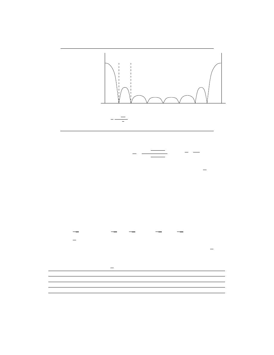
196
CHAPTER 9. FOURIER TRANSFORM
1
0
2pi/N 4pi/N
2pi
D
.
Figure 9.1:
Dirichlet sinc,
1
N
sin
(
ωN
2
)
sin
(
ω
2
)
X e
jω
=
N −1
X
k=0
(X [k])
!
1
N
sin
ωN −2πk
2
sin
ωN −2πk
2N
e
(−j)
(
ω−
2π
N
k
)
N −1
2
!
• - The DFT has a convenient matrix representation. Defining W
N
= e
(−j)
2π
N
,
X [0]
X [1]
..
.
X [N − 1]
=
W
0
N
W
0
N
W
0
N
W
0
N
. . .
W
0
N
W
1
N
W
2
N
W
3
N
. . .
W
0
N
W
2
N
W
4
N
W
6
N
. . .
..
.
..
.
..
.
..
.
..
.
x [0]
x [1]
..
.
x [N − 1]
(9.5)
where X = W (x) respectively. W has the following properties:
– - W is Vandermonde: the nth column of W is a polynomial in W
n
N
– - W is symmetric: W = W
T
– -
1
√
N
W is unitary:
1
√
N
W
1
√
N
W
H
=
1
√
N
W
H
1
√
N
W
= I
– -
1
N
W
∗
= W
−1
, the IDFT matrix.
• - For N a power of 2, the FFT can be used to compute the DFT using about
N
2
log
2
N
rather than N
2
operations.
N
N
2
log
2
N
N
2
16
32
256
64
192
4096
256
1024
65536
1024
5120
1048576
10.2 Discrete Fourier Transform (DFT)
The discrete-time Fourier transform (and the continuous-time transform as well) can be
evaluated when we have an analytic expression for the signal. Suppose we just have a signal,

197
such as the speech signal used in the previous chapter, for which there is no formula. How
then would you compute the spectrum? For example, how did we compute a spectrogram
such as the one shown in the speech signal example (pg ??)? The Discrete Fourier Transform
(DFT) allows the computation of spectra from discrete-time data. While in discrete-time
we can exactly calculate spectra, for analog signals no similar exact spectrum computation
exists. For analog-signal spectra, use must build special devices, which turn out in most
cases to consist of A/D converters and discrete-time computations. Certainly discrete-time
spectral analysis is more flexible than continuous-time spectral analysis.
The formula for the DTFT (pg ??) is a sum, which conceptually can be easily computed
save for two issues.
• - Signal duration. The sum extends over the signal’s duration, which must be finite
to compute the signal’s spectrum. It is exceedingly difficult to store an infinite-length
signal in any case, so we’ll assume that the signal extends over [0, N − 1].
• - Continuous frequency. Subtler than the signal duration issue is the fact that the
frequency variable is continuous: It may only need to span one period, like
−
1
2
,
1
2
or [0, 1], but the DTFT formula as it stands requires evaluating the spectra at all
frequencies within a period. Let’s compute the spectrum at a few frequencies; the
most obvious ones are the equally spaced ones f =
k
K
, k ∈ {k, . . . , K − 1}.
We thus define the discrete Fourier transform (DFT) to be
∀k, k ∈ {0, . . . , K − 1} : S (k) =
N −1
X
n=0
s (n) e
−
(
j2πnk
K
)
(9.6)
Here, S (k) is shorthand for S
e
j2π
k
K
.
We can compute the spectrum at as many equally spaced frequencies as we like. Note
that you can think about this computationally motivated choice as sampling the spectrum;
more about this interpretation later. The issue now is how many frequencies are enough to
capture how the spectrum changes with frequency. One way of answering this question is
determining an inverse discrete Fourier transform formula: given S (k), k = {0, . . . , K − 1}
how do we find s (n), n = {0, . . . , N − 1}? Presumably, the formula will be of the form
s (n) =
P
K−1
k=0
S (k) e
j2πnk
K
.
Substituting the DFT formula in this prototype inverse
transform yields
s (n) =
K−1
X
k=0
N −1
X
m=0
s (m) e
−
(
j
2πmk
K
)e
j
2πnk
K
!
(9.7)
Note that the orthogonality relation we use so often has a different character now.
K−1
X
k=0
e
−
(
j
2πkm
K
)e
j
2πkn
K
=
K if m = {n, (n ± K) , (n ± 2K) , . . . }
0 otherwise
(9.8)
We obtain nonzero value whenever the two indices differ by multiples of K. We can express
this result as K
P
l
(δ (m − n − lK)). Thus, our formula becomes
s (n) =
N −1
X
m=0
s (m) K
∞
X
l=−∞
(δ (m − n − lK))
!
(9.9)
The integers n and m both range over {0, . . . , N − 1}. To have an inverse transform, we
need the sum to be a single unit sample for m, n in this range. If it did not, then s (n)

198
CHAPTER 9. FOURIER TRANSFORM
would equal a sum of values, and we would not have a valid transform: Once going into the
frequency domain, we could not get back unambiguously! Clearly, the term l = 0 always
provides a unit sample (we’ll take care of the factor of K soon). If we evaluate the spectrum
at fewer frequencies than the signal’s duration, the term corresponding to m = n + K
will also appear for some values of m, n = {0, . . . , N − 1}. This situation means that our
prototype transform equals s (n)+s (n + K) for some values of n. The only way to eliminate
this problem is to require K ≥ N : We must have more frequency samples than the signal’s
duration. In this way, we can return from the frequency domain we entered via the DFT.
Exercise 9.1:
When we have fewer frequency samples than the signal’s duration, some discrete-
time signal values equal the sum of the original signal values. Given the sampling
interpretation of the spectrum, characterize this effect a different way.
Solution:
This situation amounts to aliasing in the time-domain.
Another way to understand this requirement is to use the theory of linear equations. If
we write out the expression for the DFT as a set of linear equations,
s (0) + s (1) + · · · + s (N − 1) = S (0)
(9.10)
s (0) + s (1) e
(−j)
2π
K
+ · · · + s (N − 1) e
(−j)
2π(N −1)
K
= S (1)
..
.
s (0) + s (1) e
(−j)
2π(K−1)
K
+ · · · + s (N − 1) e
(−j)
2π(N −1)(K−1)
K
= S (K − 1)
we have K equations in N unknowns if we want to find the signal from its sampled spectrum.
This requirement is impossible to fulfill if K < N ; we must have K ≥ N . Our orthogonality
relation essentially says that if we have a sufficient number of equations (frequency samples),
the resulting set of equations can indeed be solved.
By convention, the number of DFT frequency values K is chosen to equal the signal’s
duration N . The discrete Fourier transform pair consists of
Discrete Fourier Transform Pair
S (k) =
N −1
X
n=0
s (n) e
−
(
j
2πnk
N
)
(9.11)
s (n) =
1
N
N −1
X
k=0
S (k) e
j
2πnk
N
(9.12)

199
10.3 Table of Common Fourier Transforms
Time Domain Signal
Frequency Domain Signal
Condition
e
−(at)
u (t)
1
a+jω
a > 0
e
at
u (−t)
1
a−jω
a > 0
e
−(a|t|)
2a
a
2
+ω
2
a > 0
te
−(at)
u (t)
1
(a+jω)
2
a > 0
t
n
e
−(at)
u (t)
n!
(a+jω)
n+1
a > 0
δ (t)
1
1
2πδ (ω)
e
jω
0
t
2πδ (ω − ω
0
)
cos (ω
0
t)
π (δ (ω − ω
0
) + δ (ω + ω
0
))
sin (ω
0
t)
jπ (δ (ω + ω
0
) − δ (ω − ω
0
))
u (t)
πδ (ω) +
1
jω
sgn (t)
2
jω
cos (ω
0
t) u (t)
π
2
(δ (ω − ω
0
) + δ (ω + ω
0
))+
jω
ω
0
2
−ω
2
sin (ω
0
t) u (t)
π
2j
(δ (ω − ω
0
) − δ (ω + ω
0
))+
ω
0
ω
0
2
−ω
2
e
−(at)
sin (ω
0
t) u (t)
ω
0
(a+jω)
2
+ω
0
2
a > 0
e
−(at)
cos (ω
0
t) u (t)
a+jω
(a+jω)
2
+ω
0
2
a > 0
u (t + τ ) − u (t − τ )
2τ
sin(ωτ )
ωτ
= 2τ sinc (ωt)
ω
0
π
sin(ω
0
t)
ω
0
t
=
ω
0
π
sinc (ω
0
)
u (ω + ω
0
) − u (ω − ω
0
)
t
τ
+ 1
u
t
τ
+ 1
− u
t
τ
+
−
t
τ
+ 1 u
t
τ
− u
t
τ
− 1
=
triag
t
2τ
τ sinc
2
ωτ
2
ω
0
2π
sinc
2
ω
0
t
2
ω
ω
0
+ 1
u
ω
ω
0
+ 1
− u
ω
ω
0
+
−
ω
ω
0
+ 1
u
ω
ω
0
− u
ω
ω
0
− 1
=
triag
ω
2ω
0
P
∞
n=−∞
(δ (t − nT ))
ω
0
P
∞
n=−∞
(δ (ω − nω
0
))
ω
0
=
2π
T
e
−
t2
2σ2
σ
√
2πe
−
σ2 ω2
2
10.4 Discrete-Time Fourier Transform (DTFT)
Discrete-Time Fourier Transform
X (ω) =
∞
X
n=−∞
x (n) e
−(jωn)
(9.13)
Inverse Discrete-Time Fourier Transform
x (n) =
1
2π
Z
2π
0
X (ω) e
jωn
dω
(9.14)
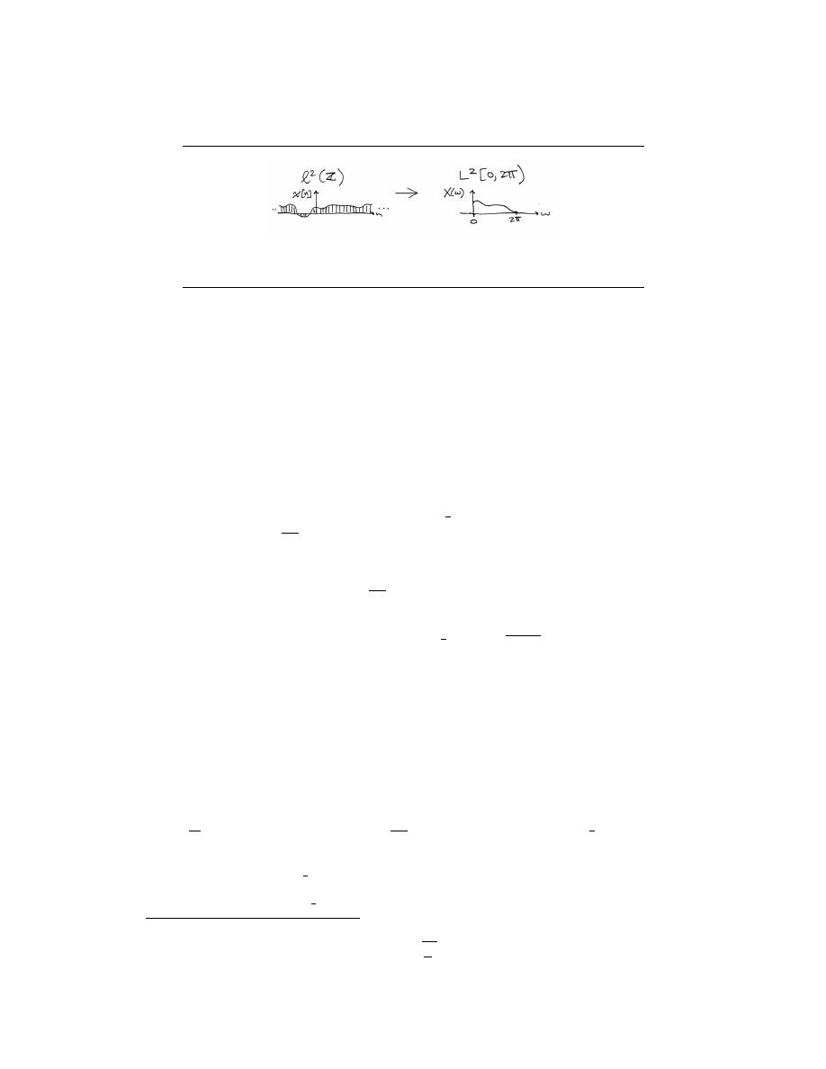
200
CHAPTER 9. FOURIER TRANSFORM
Figure 9.2:
Mapping l
2
(Z) in the time domain to L
2
([0, 2π)) in the frequency domain.
9.4.1 Relevant Spaces
The Discrete-Time Fourier Transform maps infinite-length, discrete-time signals in l
2
to
finite-length (or 2π-periodic), continuous-frequency signals in L
2
.
10.5 Discrete-Time Fourier Transform Properties
10.6 Discrete-Time Fourier Transform Pair
When we obtain the discrete-time signal via sampling an analog signal, the Nyquist fre-
quency corresponds to the discrete-time frequency
1
2
. To show this, note that a sinusoid at
the Nyquist frequency
1
2T
s
has a sampled waveform that equals
Sinusoid at Nyquist Freqency 1/2T
cos
2π
1
2T
s
nT
s
=
cos (πn)
=
(−1)
n
(9.15)
The exponential in the DTFT at frequency
1
2
equals e
−(j2πn)
2
= e
−(jπn)
= (−1)
n
,
meaning that the correspondence between analog and discrete-time frequency is established:
Analog, Discrete-Time Frequency Relationship
f
D
= f
A
T
s
(9.16)
where f
D
and f
A
represent discrete-time and analog frequency variables, respectively.
The aliasing figure (pg ??) provides another way of deriving this result. As the duration
of each pulse in the periodic sampling signal p
T
s
(t) narrows, the amplitudes of the signal’s
spectral repetitions, which are governed by the Fourier series coefficients (pg ??) of p
T
s
(t)
, become increasingly equal.
1
Thus, the sampled signal’s spectrum becomes periodic with
period
1
T
s
. Thus, the Nyquist frequency
1
2T
s
corresponds to the frequency
1
2
.
The inverse discrete-time Fourier transform is easily derived from the following relation-
ship:
Z
1
2
−
(
1
2
)
e
−(j2πf m)
e
+jπf n
df =
1 if m = n
0 if m 6= n
(9.17)
1
Examination of the periodic pulse signal (pg ??) reveals that as ∆ decreases, the value of c
0
, the
largest Fourier coefficient, decreases to zero: |c
0
| =
A∆
T
.
Thus, to maintain a mathematically viable
Sampling Theorem, the amplitude A must increase as
1
∆
, becoming infinitely large as the pulse duration
decreases. Practical systems use a small value of ∆ , say 0.1T
s
and use amplifiers to rescale the signal.

201
Discrete-Time Fourier Transform Properties
Sequence Domain
Frequency Domain
Linearity
a
1
s
1
(n) + a
2
s
2
(n)
a
1
S
1
e
j2πf
+ a
2
S
2
e
j2πf
Conjugate Symmetry
s (n) real
S e
j2πf
= S e
−(j2πf )
∗
Even Symmetry
s (n) = s (−n)
S e
j2πf
= S e
−(j2πf )
Odd Symmetry
s (n) = − (s (−n))
S e
j2πf
=
− S e
−(j2πf )
Time Delay
s (n − n
0
)
e
−(j2πf n
0
)
S e
j2πf
Complex Modulation
e
j2πf
0
n
s (n)
S e
j2π(f −f
0
)
Amplitude Modulation
s (n) cos (2πf
0
n)
S
(
e
j2π(f −f0)
)
+S
(
e
j2π(f +f0)
)
2
s (n) sin (2πf
0
n)
S
(
e
j2π(f −f0)
)
−S
(
e
j2π(f +f0)
)
2j
Multiplication by n
ns (n)
1
−(2jπ)
d
df
S e
j2πf
Sum
P
∞
n=−∞
(s (n))
S e
j2π0
Value at Origin
s (0)
R
1
2
−
(
1
2
)
S e
j2πf
df
Parseval’s Theorem
P
∞
n=−∞
(|s (n) |)
2
R
1
2
−
(
1
2
)
|S e
j2πf
|
2
df
Figure 9.3: Discrete-time Fourier transform properties and relations.

202
CHAPTER 9. FOURIER TRANSFORM
Therefore, we find that
R
1
2
−
(
1
2
)
S e
j2πf
e
+j2πf n
df
=
R
1
2
−
(
1
2
)
P
m
s (m) e
−(j2πf m)
e
+j2πf n
df
=
P
m
s (m)
R
1
2
−
(
1
2
)
e
(−(j2πf ))(m−n)
df
=
s (n)
(9.18)
The Fourier transform pairs in discrete-time are
Fourier Transform Pairs in Discrete Time
S e
j2πf
=
X
n
s (n) e
−(j2πf n)
(9.19)
Fourier Transform Pairs in Discrete Time
s (n) =
Z
1
2
−
(
1
2
)
S e
j2πf
e
+j2πf n
df
(9.20)
10.7 DTFT Examples
Example 9.1:
Let’s compute the discrete-time Fourier transform of the exponentially decaying
sequence s (n) = a
n
u (n) , where u (n) is the unit-step sequence. Simply plugging
the signal’s expression into the Fourier transform formula,
Fourier Transform Formula
S e
j2πf
=
P
∞
n=−∞
a
n
u (n) e
−(j2πf n)
=
P
∞
n=0
ae
−(j2πf )
n
(9.21)
This sum is a special case of the geometric series .
Geometric Series
∀α, |α| < 1 :
∞
X
n=0
(α
n
) =
1
1 − α
(9.22)
Thus, as long as |a| < 1 , we have our Fourier transform.
S e
j2πf
=
1
1 − ae
−(j2πf )
(9.23)
Using Euler’s relation, we can express the magnitude and phase of this spectrum.
|S e
j2πf
| =
1
q
(1 − acos (2πf ))
2
+ a
2
sin
2
(2πf )
(9.24)
∠ S e
j2πf
= −
arctan
asin (2πf )
1 − acos (2πf )
(9.25)
No matter what value of a we choose, the above formulae clearly demonstrate the
periodic nature of the spectra of discrete-time signals. Figure 9.4 shows indeed that
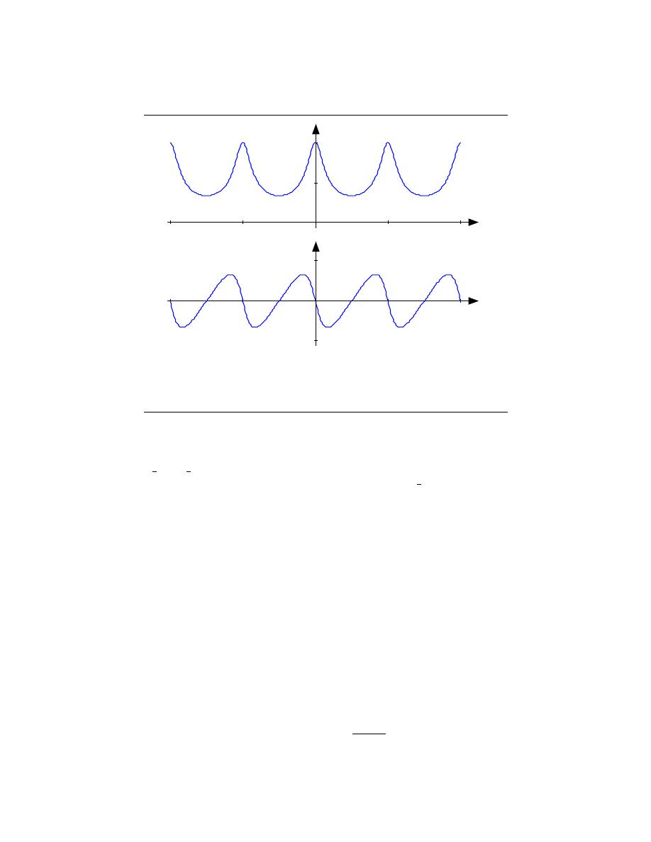
203
-2
-1
0
1
2
1
2
f
|S(e
j2
π
f
)|
-2
-1
1
2
-45
45
f
∠
S(e
j2
π
f
)
Figure 9.4:
The spectrum of the exponential signal (a = 0.5) is shown over the
frequency range [−2, 2], clearly demonstrating the periodicity of all discrete-time spectra.
The angle has units of degrees.
the spectrum is a periodic function. We need only consider the spectrum between
−
1
2
and
1
2
to unambiguously define it. When a > 0 , we have a lowpass spectrum
– the spectrum diminishes as frequency increases from 0 to
1
2
– with increasing a
leading to a greater low frequency content; for a < 0 , we have a highpass spectrum
(Figure 9.5).
Example 9.2:
Analogous to the analog pulse signal, let’s find the spectrum of the length- N pulse
sequence.
s (n) =
1 if 0 ≤ n ≤ N − 1
0 otherwise
(9.26)
The Fourier transform of this sequence has the form of a truncated geometric series.
S e
j2πf
=
N −1
X
n=0
e
−(j2πf n)
(9.27)
For the so-called finite geometric series, we know that
Finite Geometric Series
N +n
0
−1
X
n=n
0
(α
n
) = α
n
0
1 − α
N
1 − α
(9.28)
for all values of α .
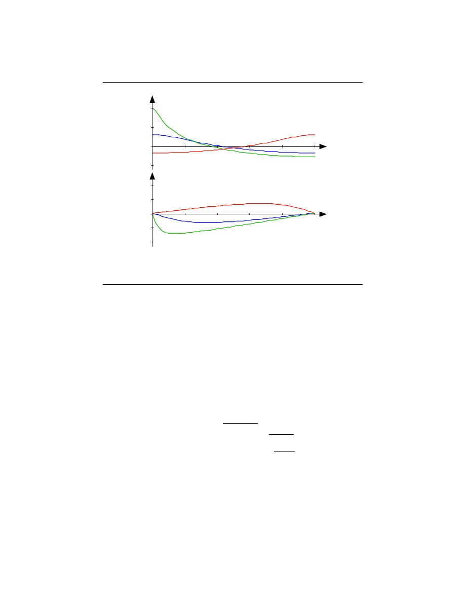
204
CHAPTER 9. FOURIER TRANSFORM
f
a = 0.9
a = 0.5
a = –0.5
Spectral Magnitude (dB)
-10
0
10
20
0.5
a = 0.9
a = 0.5
a = –0.5
Angle (degrees)
f
-90
-45
0
45
90
0.5
Figure 9.5:
The spectra of several exponential signals are shown. What is the apparent
relationship between the spectra for a = 0.5 and a = −0.5 ?
Exercise 9.2:
Derive this formula for the finite geometric series sum. The ”trick” is to consider
the difference between the series’; sum and the sum of the series multiplied by α .
Solution:
α
N +n
0
−1
X
n=n
0
(α
n
) −
N +n
0
−1
X
n=n
0
(α
n
) = α
N +n
0
− α
n
0
(9.29)
which, after manipulation, yields the geometric sum formula.
Applying this result yields (Figure 9.6.)
S e
j2πf
=
1−e
−(j2πf N )
1−e
−(j2πf )
=
e
(−(jπf ))(N −1) sin(πf N )
sin(πf )
(9.30)
The ratio of sine functions has the generic form of
sin(N x)
sin(x)
, which is known as the
discrete-time sinc function , dsinc (x) . Thus, our transform can be concisely expressed
as S e
j2πf
= e
(−(jπf ))(N −1)
dsinc (πf ) . The discrete-time pulse’s spectrum contains many
ripples, the number of which increase with N , the pulse’s duration.
10.8 Continuous-Time Fourier Transform (CTFT)
9.8.1 Introduction
Due to the large number of continuous-time signals that are present, the Fourier series
provided us the first glimpse of how me we may represent some of these signals in a general
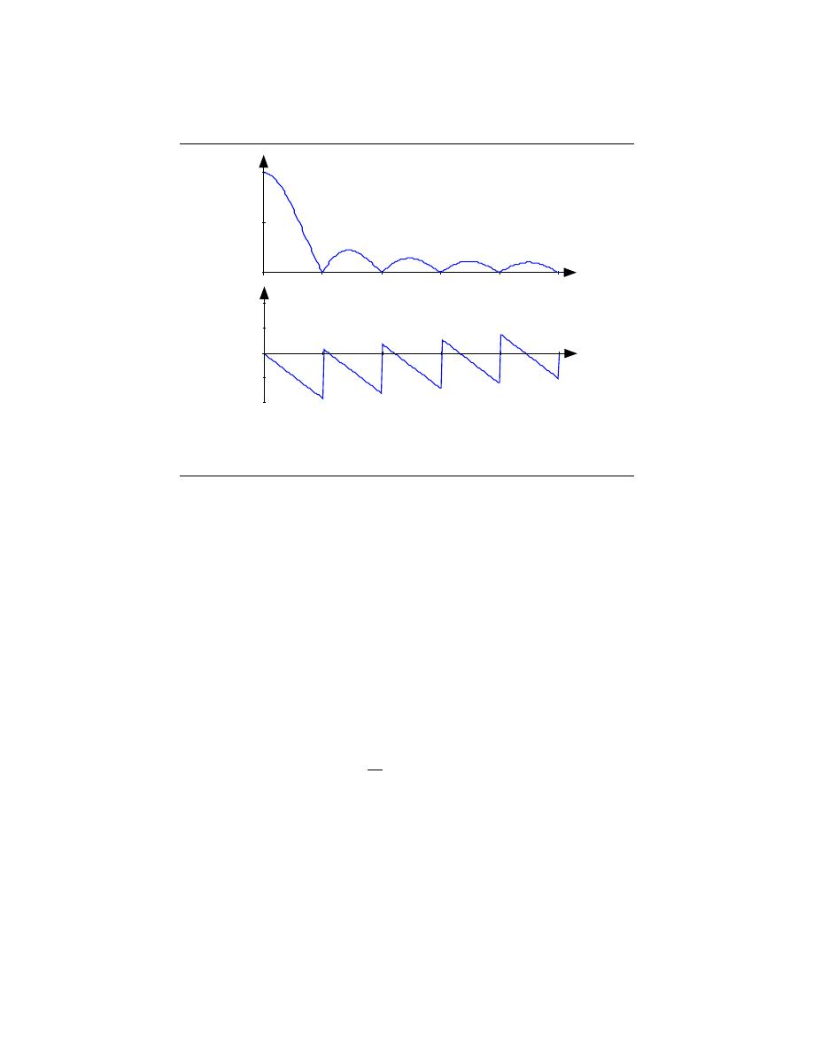
205
f
0
5
10
Spectral Magnitude
0.5
-180
-90
0
90
180
f
0.5
Angle (degrees)
Figure 9.6:
The spectrum of a length-ten pulse is shown. Can you explain the rather
complicated appearance of the phase?
manner: as a superpostion of a number of sinusoids. Now, we can look at a way to represent
continuous-time nonperiodic signals using the same idea of superposition. Below we will
present the Continuous-Time Fourier Transform (CTFT), also referred to as just the
Fourier Transform (FT). Because the CTFT now deals with nonperiodic signals, we must
now find a way to include all frequencies in the general equations.
9.8.1.1 Equations
Continuous-Time Fourier Transform
F (Ω) =
Z
∞
−∞
f (t) e
−(jΩt)
dt
(9.31)
Inverse CTFT
f (t) =
1
2π
Z
∞
−∞
F (Ω) e
jΩt
dΩ
(9.32)
warning:
Do not be confused by notation - it is not uncommon to see the above
formula written slightly different. One of the most common differences among
many professors is the way that the exponential is written. Above we used the
radial frequency variable Ω in the exponential, where Ω = 2πf , but one will often
see professors include the more explicit expression, j2πf t, in the exponential. Click
here for an overview of the notation used in Connexion’s DSP modules.
The above equations for the CTFT and its inverse come directly from the Fourier series
and our understanding of its coefficients. For the CTFT we simply utilize integration rather
than summation to be able to express the aperiodic signals. This should make sense since

206
CHAPTER 9. FOURIER TRANSFORM
Figure 9.7:
Mapping L
2
(R) in the time domain to L
2
(R) in the frequency domain.
for the CTFT we are simply extending the ideas of the Fourier series to include nonperiodic
signals, and thus the entire frequency spectrum. Look at the Derivation of the Fourier
Transform for a more indepth look at this.
9.8.2 Relevant Spaces
The Continuous-Time Fourier Transform maps infinite-length, continuous-time signals in
L
2
to infinite-length, continuous-frequency signals in L
2
. Review the Fourier Analysis for
an overview of all the spaces used in Fourier analysis.
For more information on the characteristics of the CTFT, please look at the module on
Properties of the Fourier Transform.
9.8.3 Example Problems
Exercise 9.3:
Find the Fourier Transform (CTFT) of the function
f (t) =
e
−(αt)
if t ≥ 0
0 otherwise
(9.33)
Solution:
In order to calculate the Fourier transform, all we need to use is Equation 9.31,
complex exponentials, and basic calculus.
F (Ω)
=
R
∞
−∞
f (t) e
−(jΩt)
dt
=
R
∞
0
e
−(αt)
e
−(jΩt)
dt
=
R
∞
0
e
(−t)(α+jΩ)
dt
=
0 −
−1
α+jΩ
(9.34)
F (Ω) =
1
α + jΩ
(9.35)
Exercise 9.4:
Find the inverse Fourier transform of the square wave defined as
X (Ω) =
1 if |Ω| ≤ M
0 otherwise
(9.36)

207
Solution:
Here we will use Equation 9.32 to find the inverse FT given that t 6= 0.
x (t)
=
1
2π
R
M
−M
e
jΩt
dΩ
=
1
2π
e
jΩt
|
Ω,Ω=e
jw
=
1
πt
sin (M t)
(9.37)
x (t) =
M
π
sinc
M t
π
(9.38)
10.9 Properties of the Continuous-Time Fourier Trans-
form
This module will look at some of the basic properties of the Continuous-Time Fourier Trans-
form (CTFT). The first section contains a table that illustrates the properties, and the
sections following it discuss a few of the more interesting properties in more depth. In the
table, click on the operation name to be taken to the properties explanation found later on
this page. Look at this module for an expanded table of more Fourier transform properties.
note:
We will be discussing these properties for aperiodic, continuous-time sig-
nals but understand that very similar properites hold for discrete-time signals and
periodic signals as well.
9.9.1 Table of CTFT Properties
Operation Name
Signal ( f (t) )
Transform ( F (ω) )
Addition (Section 9.9.2.1)
f
1
(t) + f
2
(t)
F
1
(ω) + F
2
(ω)
Scalar Multiplication (Sec-
tion 9.9.2.1)
αf (t)
αF (t)
Symmetry (Section 9.9.2.2)
F (t)
2πf (−ω)
Time
Scaling
(Sec-
tion 9.9.2.3)
f (αt)
1
|α|
F
ω
α
Time Shift (Section 9.9.2.4)
f (t − τ )
F (ω) e
−(jωτ )
Modulation
(Frequency
Shift) (Section 9.9.2.5)
f (t) e
jωφ
F (ω − φ)
Convolution in Time (Sec-
tion 9.9.2.6)
(f
1
(t) , f
2
(t))
F
1
(t) F
2
(t)
Convolution in Frequency
(Section 9.9.2.6)
f
1
(t) f
2
(t)
1
2π
(F
1
(t) , F
2
(t))
Differentiation
(Sec-
tion 9.9.2.7)
d
n
dt
n
f (t)
(jω)
n
F (ω)
9.9.2 Discussion of Fourier Transform Properties
After glancing at the above table and getting a feel for the properties of the CTFT, we
will now take a little more time to discuss some of the more interesting, and more useful,
properties.

208
CHAPTER 9. FOURIER TRANSFORM
9.9.2.1 Linearity
The combined addition and scalar multiplication properties in the table above demonstrate
the basic property of linearity. What you should see is that if one takes the Fourier transform
of a linear combination of signals then it will be the same as the linear combination of the
Fourier transforms of each of the individual signals. This is crucial when using a table of
transforms to find the transform of a more complicated signal.
Example 9.3:
We will begin with the following signal:
z (t) = αf
1
(t) + αf
2
(t)
(9.39)
Now, after we take the Fourier transform, shown in the equation below, notice that
the linear combination of the terms is unaffected by the transform.
Z (ω) = αF
1
(ω) + αF
2
(ω)
(9.40)
9.9.2.2 Symmetry
Symmetry is a property that can make life quite easy when solving problems involving
Fourier transforms. Basically what this property says is that since a rectangular function
in time is a sinc function in frequency, then a sinc fucntion in time will be a rectangular
function in frequency. This is a direct result of the similarity between the forward CTFT
and the inverse CTFT. The only difference is the scaling by 2π and a frequency reversal.
9.9.2.3 Time Scaling
This property deals with the effect on the frequency-domain representation of a signal if the
time variable is altered. The most important concept to understand for the time scaling
property is that signals that are narrow in time will be broad in frequency and vice versa.
The simplest example of this is a delta function, a unit pulse (pg ??) with a very small
duration, in time that becomes an infinite-length constant function in frequency.
The table above shows this idea for the general transformation from the time-domain
to the frequency-domain of a signal. You should be able to easily notice that these equa-
tions show the relationship mentioned previously: if the time variable is increased then the
frequency range will be decreased.
9.9.2.4 Time Shifting
Time shifting shows that a shift in time is equivalent to a linear phase shift in frequency.
Since the frequency content depends only on the shape of a signal, which is unchanged in a
time shift, then only the phase spectrum will be altered. This property can be easily proved
using the Fourier Transform, so we will show the basic steps below:
Example 9.4:
We will begin by letting z (t) = f (t − τ ). Now let us take the Fourier transform
with the previous expression substitued in for z (t).
Z (ω) =
Z
∞
−∞
f (t − τ ) e
−(jωt)
dt
(9.41)

209
Now let us make a simple change of variables, where σ = t − τ . Through the
calculations below, you can see that only the variable in the exponential are altered
thus only changing the phase in the frequency domain.
Z (ω)
=
R
∞
−∞
f (σ) e
−(jω(σ+τ )t)
dτ
=
e
−(jωτ )
R
∞
−∞
f (σ) e
−(jωσ)
dσ
=
e
−(jωτ )
F (ω)
(9.42)
9.9.2.5 Modulation (Frequency Shift)
Modulation is absolutely imperative to communications applications. Being able to shift a
signal to a different frequency, allows us to take advantage of different parts of the electro-
magnetic spectrum is what allows us to transmit television, radio and other applications
through the same space without significant interference.
The proof of the frequency shift property is very similar to that of the time shift (Sec-
tion 9.9.2.4); however, here we would use the inverse Fourier transform in place of the Fourier
transform. Since we went through the steps in the previous, time-shift proof, below we will
just show the initial and final step to this proof:
z (t) =
1
2π
Z
∞
−∞
F (ω − φ) e
jωt
dω
(9.43)
Now we would simply reduce this equation through another change of variables and simplify
the terms. Then we will prove the property experssed in the table above:
z (t) = f (t) e
jφt
(9.44)
9.9.2.6 Convolution
Convolution is one of the big reasons for converting signals to the frequency domain, since
convolution in time becomes multiplication in frequency. This property is also another
excellent example of symmetry between time and frequency. It also shows that there may
be little to gain by changing to the frequency domain when multiplication in time is involved.
We will introduce the convolution integral here, but if you have not seen this before or
need to refresh your memory, then look at the continuous-time convolution module for a
more in depth explanation and derivation.
y (t)
=
(f
1
(t) , f
2
(t))
=
R
∞
−∞
f
1
(τ ) f
2
(t − τ ) dτ
(9.45)
9.9.2.7 Time Differentiation
Since LTI systems can be represented in terms of differential equations, it is apparent with
this property that converting to the frequency domain may allow us to convert these com-
plicated differential equations to simpler equations involving multiplication and addition.
This is often looked at in more detail during the study of the Laplace Transform.

210
CHAPTER 9. FOURIER TRANSFORM

Chapter 10
Sampling Theorem
11.1 Sampling
10.1.1 Introduction
The digital computer can process discrete time signals using extremely flexible and pow-
erful algorithms. However, most signals of interest are continous time , which is how the
almost always appear in nature.
This module introduces the idea of translating continous time problems into discrete
time, and you can read on to learn more of the details and importance of sampling .
Key Questions
• - How do we turn a continous time signal into a discrete time signal (sampling, A/D)?
• - When can we reconstruct a CT signal exactly from its samples (reconstruction,
D/A)?
• - Manipulating the DT signal does what to the reconstructed signal?
10.1.2 Sampling
Sampling (and reconstruction) are best understood in the frequency domain. We’ll start by
looking at some examples
Exercise 10.1:
What CT signal f (t) has the CTFT shown below?
f (t) =
1
2π
Z
∞
−∞
F (jw) e
jwt
dw
Hint: F (jw) = F
1
(jw) ∗ F
2
(jw) where the two parts of F (jw) are:
Solution:
f (t) =
1
2π
Z
∞
−∞
F (jw) e
jwt
dw
211
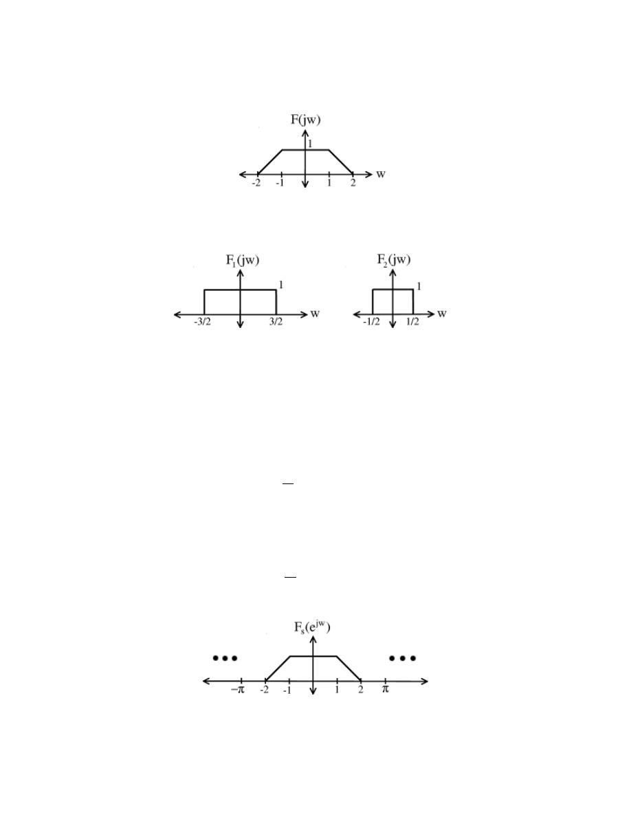
212
CHAPTER 10. SAMPLING THEOREM
Figure 10.1:
The CTFT of f (t).
(a)
(b)
Figure 10.2
Exercise 10.2:
What DT signal f
s
[n] has the DTFT shown below?
f
s
[n] =
1
2π
Z
π
−π
f
s
e
jw
e
jwn
dw
Solution:
Since F (jw) = 0 outside of [−2, 2]
f (t) =
1
2π
Z
2
−2
F (jw) e
jwt
dw
Figure 10.3:
DTFT that is a periodic (with period = 2π) version of F (jw) in Fig-
ure 10.1.
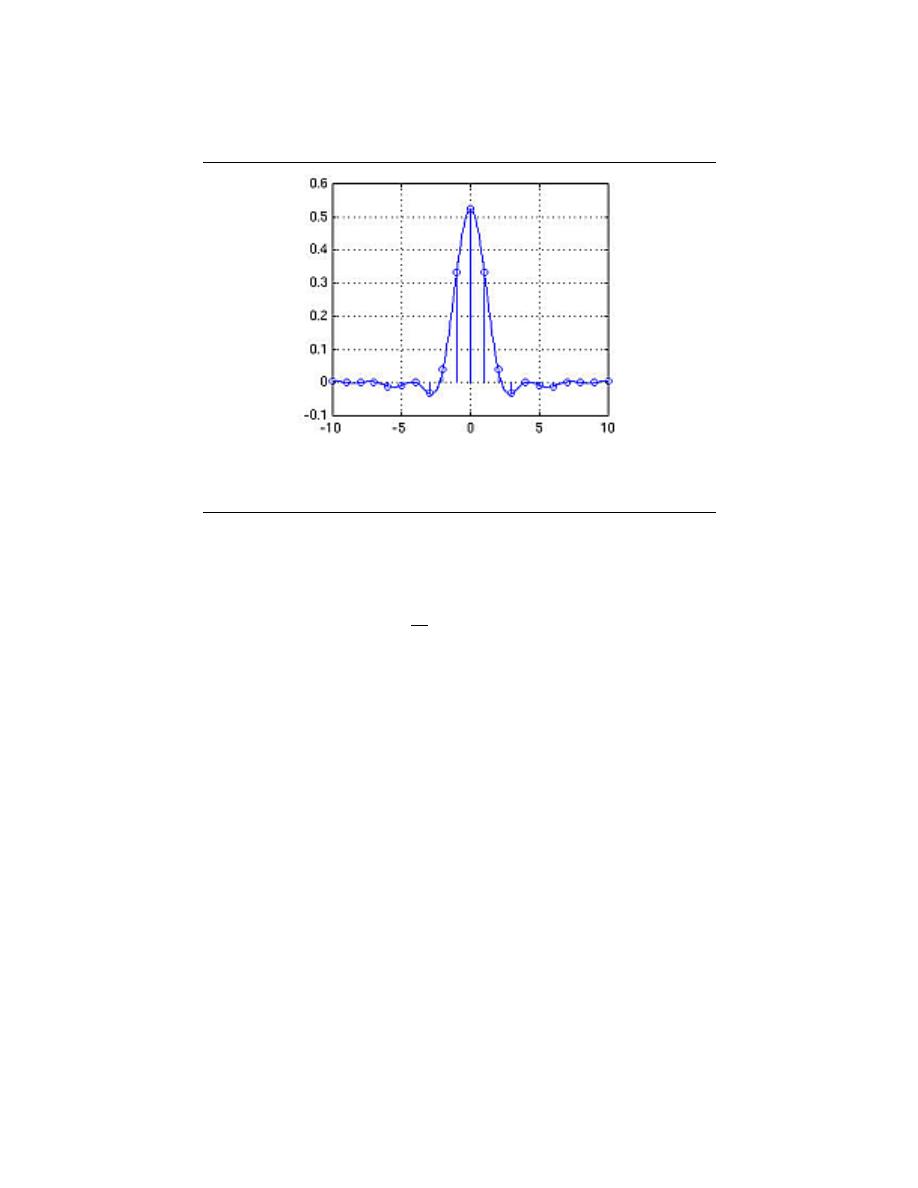
213
Figure 10.4:
f (t) is the continuous-time signal above and f
s
[n] is the discrete-time,
sampled version of f (t)
Also, since we only use one interval to reconstruct f
s
[n] from its DTFT, we have
f
s
[n] =
1
2π
Z
2
−2
f
s
e
jw
e
jwn
dw
Since F (jw) = F
s
e
jw
on [−2, 2]
f
s
[n] = f (t) |
t=n
i.e. f
s
[n] is a sampled version of f (t).
10.1.2.1 Generalization
Of course, the results from the above examples can be generalized to any f (t) with F (jw) =
0, |w| > π, where f (t) is bandlimited to [−π, π].
F
s
e
jw
is a periodic (with period 2π) version of F (jw). F
s
e
jw
is the DTFT of signal
sampled at the integers. F (jw) is the CTFT of signal.
conclusion:
If f (t) is bandlimited to [−π, π] then the DTFT of the sampled
version
f
s
[n] = f (n)
is just a periodic (with period 2π) version of F (jw).
10.1.3 Turning a Discrete Signal into a Continuous Signal
Now, let’s look at turning a DT signal into a continous time signal. Let f
s
[n] be a DT
signal with DTFT F
s
e
jw
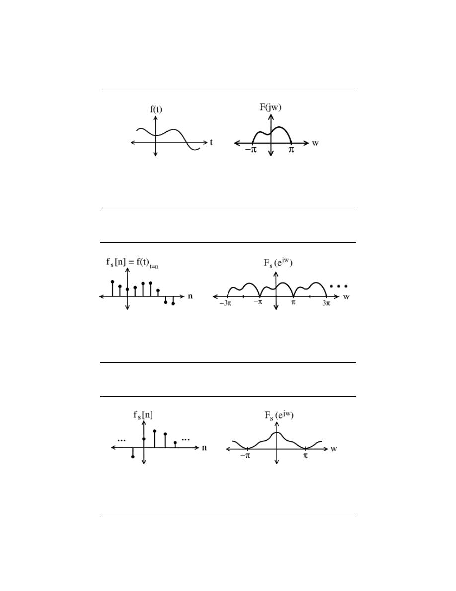
214
CHAPTER 10. SAMPLING THEOREM
(a)
(b)
Figure 10.5:
F (jw) is the CTFT of f (t).
(a)
(b)
Figure 10.6:
F
s
e
jw
is the DTFT of f
s
[n].
(a)
(b)
Figure 10.7:
F
s
e
jw
is the DTFT of f
s
[n].

215
Figure 10.8
Now, set
f
imp
(t) =
∞
X
n=−∞
(f
s
[n] δ (t − n))
The CT signal, f
imp
(t), is non-zero only on the integers where there are impluses of height
f
s
[n].
Exercise 10.3:
What is the CTFT of f
imp
(t)?
Solution:
f
imp
(t) =
∞
X
n=−∞
(f
s
[n] δ (t − n))
∼
F
imp
(jw)
=
R
∞
−∞
f
imp
(t) e
−(jwt)
dt
=
R
∞
−∞
P
∞
n=−∞
(f
s
[n] δ (t − n))
e
−(jwt)
dt
=
P
∞
n=−∞
(f
s
[n])
R
∞
−∞
δ (t − n) e
−(jwt)
dt
=
P
∞
n=−∞
(f
s
[n])
e
−(jwn)
=
F
s
e
jw
(10.1)
So, the CTFT of f
imp
(t) is equal to the DTFT of f
s
[n]
note:
We used the sifting property to show
R
∞
−∞
δ (t − n) e
−(jwt)
dt =
e
−(jwn)
Now, given the samples f
s
[n] of a bandlimited to [−π, π] signal, our next step will be to
see how we can reconstruct f (t).
11.2 Reconstruction
10.2.1 Introduction
The reconstruction process begins by taking a sampled signal, which will be in discrete time,
and performing a few operations in order to convert them into continuous-time and, with
any luck, into an exact copy of the original signal. A basic method used to reconstruct a
[−π, π] bandlimited signal from its samples on the integer is to do the following steps:
• - turn the sample sequence f
s
[n] into an impulse train f
imp
(t)
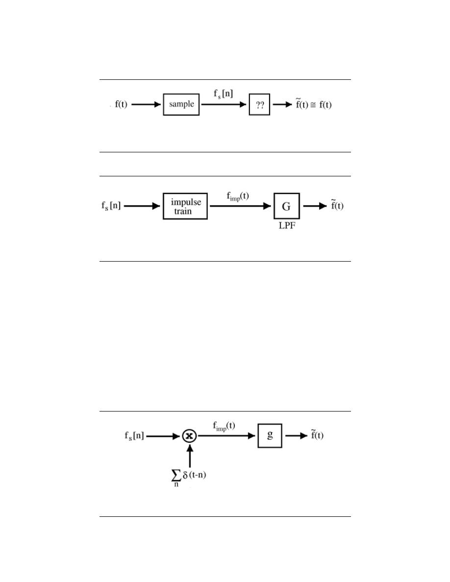
216
CHAPTER 10. SAMPLING THEOREM
Figure 10.9:
Block diagram showing the very basic steps used to reconstruct f (t).
Can we make our results equal f (t) exactly?
Figure 10.10:
Reconstruction block diagram with lowpass filter (LPF).
• - lowpass filter f
imp
(t) to get the reconstruction ˜
f (t) (cutoff freq. = π)
The lowpass filter’s impulse response is g (t). The following equations allow us to recon-
struct our signal, ˜
f (t).
˜
f (t)
=
g (t) f
imp
(t)
=
g (t)
P
∞
n=−∞
(f
s
[n] δ (t − n))
=
˜
f (t)
=
P
∞
n=−∞
(f
s
[n] (g (t) δ (t − n)))
=
P
∞
n=−∞
(f
s
[n] g (t − n))
(10.2)
Figure 10.11:
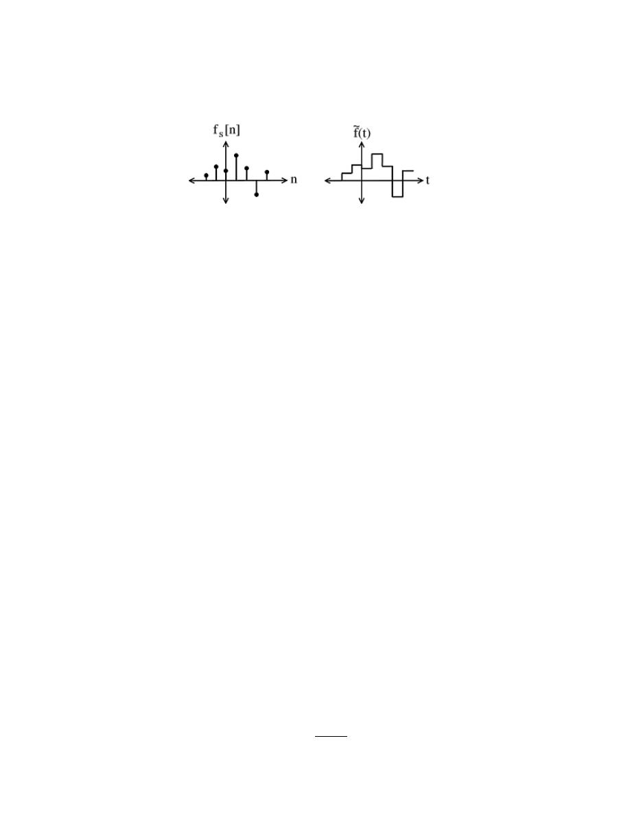
217
(a)
(b)
Figure 10.12:
Zero Order Hold
10.2.1.1 Examples of Filters g
Example 10.1:
Zero Order Hold
This type ”filter” is one of the most basic types of reconstruction filters. It simply
holds the value that is in f
s
[n] for τ seconds. This creates a block or step like
function where each value of the pulse in f
s
[n] is simply dragged over to the next
pulse. The equations and illustrations below depict how this reconstruction filter
works with the following g:
g (t) =
1 if 0 < t < τ
0 otherwise
f
s
[n] =
∞
X
n=−∞
(f
s
[n] g (t − n))
(10.3)
question:
How does ˜
f (t) reconstructed with a zero order hold compare
to the original f(t) in the frequency domain?
Example 10.2:
Nth Order Hold
Here we will look at a few quick examples of variances to the Zero Order Hold
filter discussed in the previous example.
10.2.2 Ultimate Reconstruction Filter
question:
What is the ultimate reconstruction filter?
Recall that
If G (jω) has the following shape:
then
˜
f (t) = f (t)
Therefore, an ideal lowpass filter will give us perfect reconstruction!
In the time domain, impulse response
g (t) =
sin (πt)
πt
(10.4)
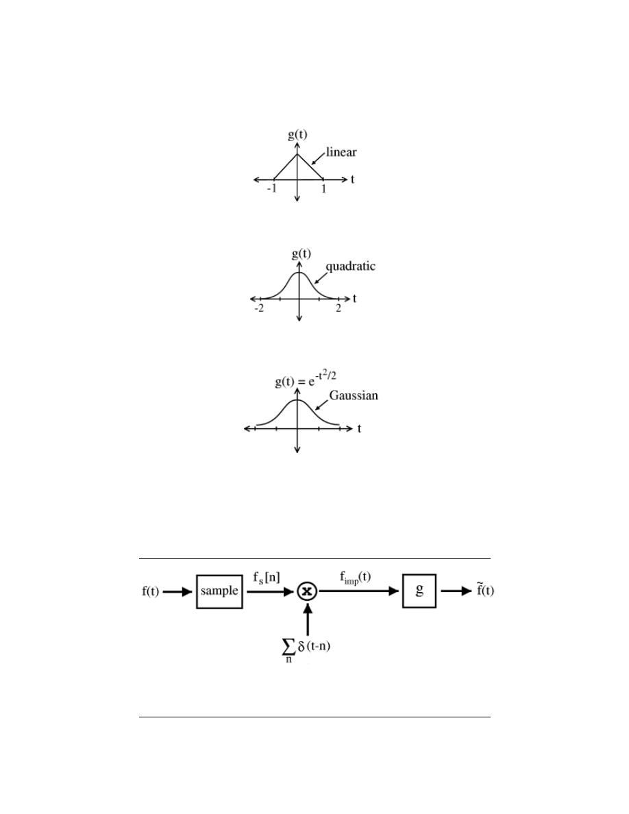
218
CHAPTER 10. SAMPLING THEOREM
(a)
(b)
(c)
Figure 10.13:
Nth Order Hold Examples (nth order hold is equal to an nth order
B-spline) (a) First Order Hold (b) Second Order Hold (c) ∞ Order Hold
Figure 10.14:
Our current reconstruction block diagram. Note that each of these
signals has its own corresponding CTFT or DTFT.
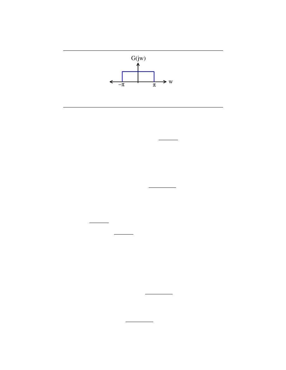
219
Figure 10.15:
Ideal lowpass filter
˜
f (t)
=
P
∞
n=−∞
(f
s
[n] g (t − n))
=
P
∞
n=−∞
f
s
[n]
sin(π(t−n))
π(t−n)
=
f (t)
(10.5)
10.2.3 Amazing Conclusions
If f(t) is bandlimited to [−π, π], it can be reconstructed perfectly from its samples on the
integers f
s
[n] = f (t) |
t=n
f (t) =
∞
X
n=−∞
f
s
[n]
sin (π (t − n))
π (t − n)
(10.6)
The above equation for perfect reconstruction deserves a closer look, which you should
continue to read in the following section to get a better understanding of reconstruction.
Here are a few things to think about for now:
• - What does
sin(π(t−n))
π(t−n)
equal at integers other than n?
• - What is the support of
sin(π(t−n))
π(t−n)
?
11.3 More on Reconstruction
10.3.1 Inroduction
In the previous module on reconstruction, we gave an introduction into how reconstruction
works and briefly derived an equation used to perfrom perfect reconstruction. Let us now
take a closer look at the perfect reconstruction formula:
f (t) =
∞
X
n=−∞
f
s
sin (π (t − n))
π (t − n)
(10.7)
We are writing f (t) in terms of shifted and scaled sinc functions.
sin (π (t − n))
π (t − n)
n∈Z
is a basis (Section 4.1.3) for the space of [−π, π] bandlimited signals. But wait . . . .

220
CHAPTER 10. SAMPLING THEOREM
10.3.1.1 Derive Reconstruction Formulas
What is
sin (π (t − n))
π (t − n)
·
sin (π (t − k))
π (t − k)
=?
(10.8)
This inner product can be hard to calculate in the time domain, so let’s use Plancharel
Theorem
· · · =
1
2π
Z
π
−π
e
−(jωn)
e
jωk
dω
(10.9)
if n = k
sinc
n
· sinc
k
=
1
2π
R
π
−π
e
−(jωn)
e
jωk
dω
=
1
(10.10)
if n 6= k
sinc
n
· sinc
k
=
1
2π
R
π
−π
e
−(jωn)
e
jωn
dω
=
1
2π
R
π
−π
e
jω(k−n)
dω
=
1
2π
sin(π(k−n))
j(k−n)
=
0
(10.11)
note:
In Equation 10.11 we used the fact that the integral of sinusoid over a
complete interval is 0 to simplify our equation.
So,
sin (π (t − n))
π (t − n)
·
sin (π (t − k))
π (t − k)
=
1 if n = k
0 if n 6= k
(10.12)
Therefore
sin (π (t − n))
π (t − n)
n∈Z
is an orthonormal basis (Section 6.7.3) (ONB) for the space of [−π, π] bandlimited functions.
sampling:
Sampling is the same as calculating ONB coefficients, which is inner
products with sincs
10.3.1.2 Summary
One last time for f (t) [−π, π] bandlimited
Synthesis
f (t) =
∞
X
n=−∞
f
s
[n]
sin (π (t − n))
π (t − n)
(10.13)
Analysis
f
s
[n] = f (t) |
t=n
(10.14)
In order to understand a little more about how we can reconstruct a signal exactly, it will
be useful to examine the relationships between the fourier transforms (CTFT and DTFT)
in more depth.
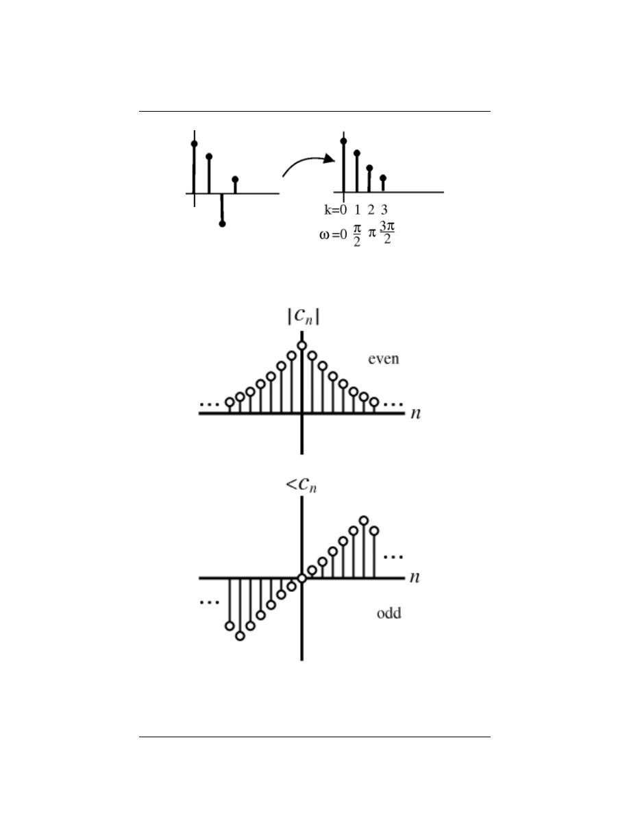
221
(a)
(b)
Figure 10.16
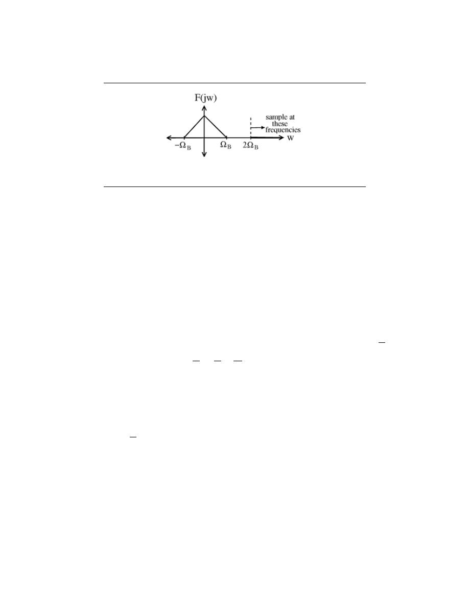
222
CHAPTER 10. SAMPLING THEOREM
Figure 10.17:
Illustration of Nyquist Frequency
11.4 Nyquist Theorem
10.4.1 Introduction
Earlier you should have been exposed to the concepts behind sampling and the sampling
theorem. While learning about these ideas, you should have begun to notice that if we
sample at too low of a rate, there is a chance that our original signal will not be uniquely
defined by our sampled signal. If this happens, then there is no garauntee that we can
correctly reconstruct the signal. As a result of this, the Nyquist Theorem was created.
Below, we will discuss just what exactly this theorem tells us.
10.4.2 Nyquist Theorem
We will let T equal our sampling period (distance between samples). Then let Ω
s
=
2π
T
(sampling frequency in radians/sec). We have seen that if f(t) is bandlimited to [−Ω
B
, Ω
B
]
and we sample with period T <
π
Ω
b
⇒
2π
Ω
s
<
π
Ω
B
⇒ Ω
s
> 2Ω
B
then we can reconstruct f(t)
from its samples.
Theorem 10.1:
Nyquist Theorem (”Fundamental Theorem of DSP”)
If f(t) is bandlimited to [−Ω
B
, Ω
B
], we can reconstruct it perfectly from its sam-
ples
f
s
[n] = f (nT )
for Ω
s
=
2π
T
> 2Ω
B
Ω
N
= 2Ω
B
is called the ”Nyquist frequency ” for f(t). For perfect reconstruction to
be possible
Ω
s
≥ 2Ω
B
where Ω
s
is sampling frequency and Ω
B
is the highest frequency in the signal.
Example 10.3:
Examples:
•- Human ear hears freqs. up to 20 KHz → CD sample rate is 44.1 KHz.
•- Phone line passes frequencies up to 4 KHz → phone company samples at 8
KHz.
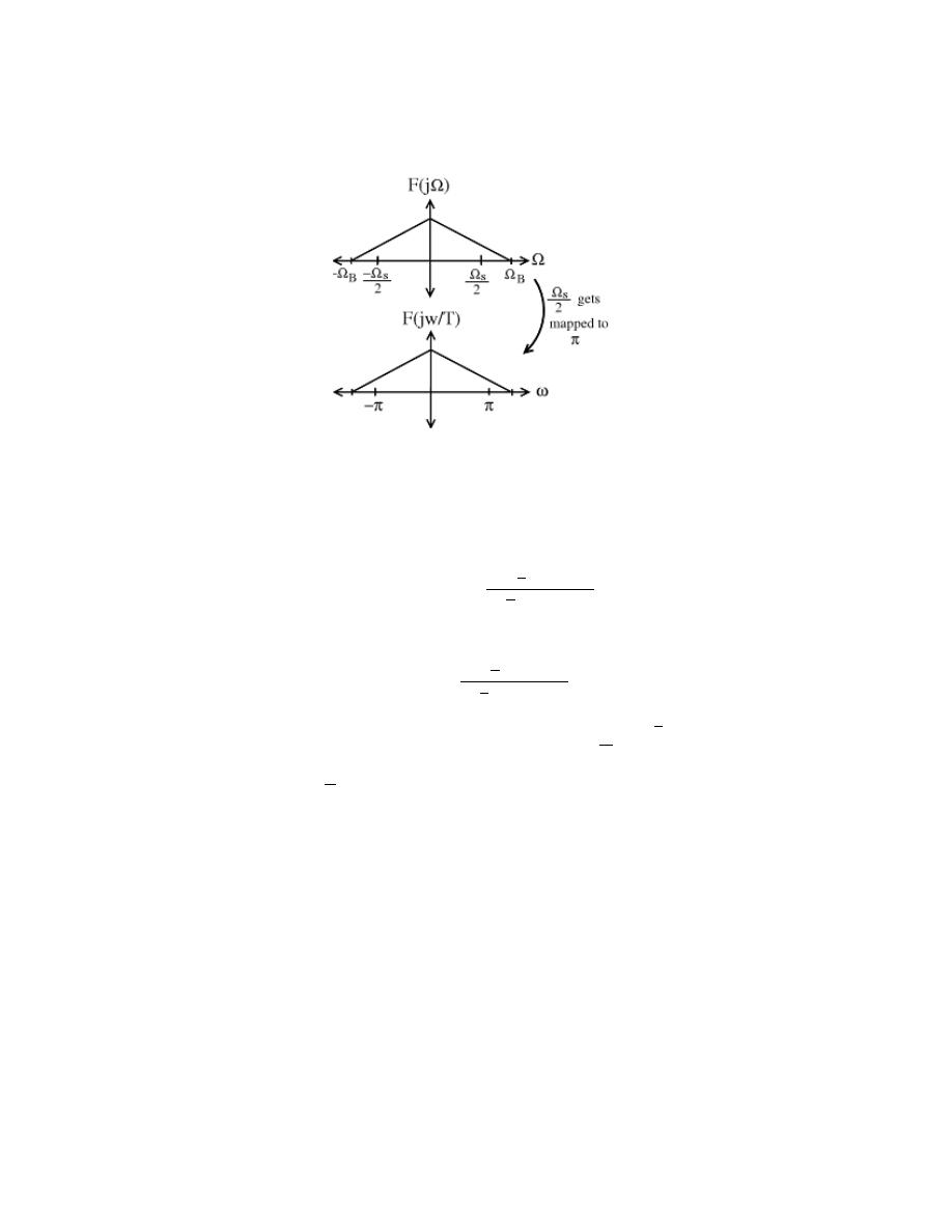
223
Figure 10.18:
10.4.2.1 Reconstruction
The reconstruction formula in the time domain looks like
f (t) =
∞
X
n=−∞
f
s
[n]
sin
π
T
(t − nT )
π
T
(t − nT )
!
We can conclude, just as before, that
∀n, n ∈ Z :
sin
π
T
(t − nT )
π
T
(t − nT )
is a basis for the space of [−Ω
B
, Ω
B
] bandlimited functions, Ω
B
=
π
T
.
The expansion
coefficient for this basis are calculated by sampling f(t) at rate
2π
T
= 2Ω
B
.
note:
The basis is also orthogonal. To make it orthonormal, we need a normal-
ization factor of
√
T .
10.4.2.2 The Big Question
Exercise 10.4:
What if Ω
s
< 2Ω
B
? What happens when we sample below the Nyquist rate?
Solution:
Go through the steps:
Finally, what will happen to F
s
e
jω
now? To answer this final question, we will
now need to look into the concept of aliasing.
11.5 Aliasing
10.5.1 Introduction
When considering the reconstruction of a signal, you should already be familiar with the
idea of the Nyquist rate. This concept allows us to find the sampling rate that will provide
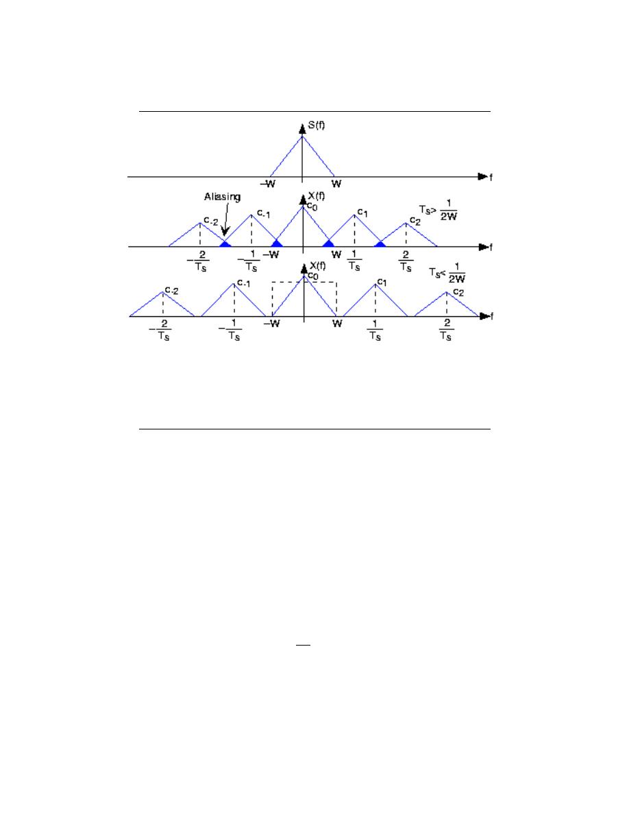
224
CHAPTER 10. SAMPLING THEOREM
Figure 10.19:
The spectrum of some bandlimited (to W Hz) signal is shown in the
top plot. If the sampling interval T
s
is chosen too large relative to the bandwidth W ,
aliasing will occur. In the bottom plot, the sampling interval is chosen sufficiently small
to avoid aliasing. Note that if the signal were not bandlimited, the component spectra
would always overlap.
for perfect reconstruction of our signal.
If we sample at too low of a rate (below the
Nyquist rate), then problems will arise that will make perfect reconstruction impossible -
this problem is known as aliasing . Aliasing occurs when there is an overlap in the shifted,
perioidic copies of our original signal’s FT, i.e. spectrum.
In the frequency domain, one will notice that part of the signal will overlap with the
periodic signals next to it. In this overlap the values of the frequency will be added together
and the shape of the signals spectrum will be unwantingly altered. This overlapping, or
aliasing, makes it impossible to correctly determine the correct strength of that frequency.
The figure belows provides a visual example of this phenomenon:
10.5.2 Aliasing and Sampling
If we sample too slowly, i.e.,
∀,
T >
π
Ω
B
: Ω
s
< 2Ω
B
We cannot recover the signal from its samples due to aliasing.
Example 10.4:
Let f
1
(t) have CTFT.
Let f
2
(t) have CTFT.
Try to sketch and answer the following questions on your own:
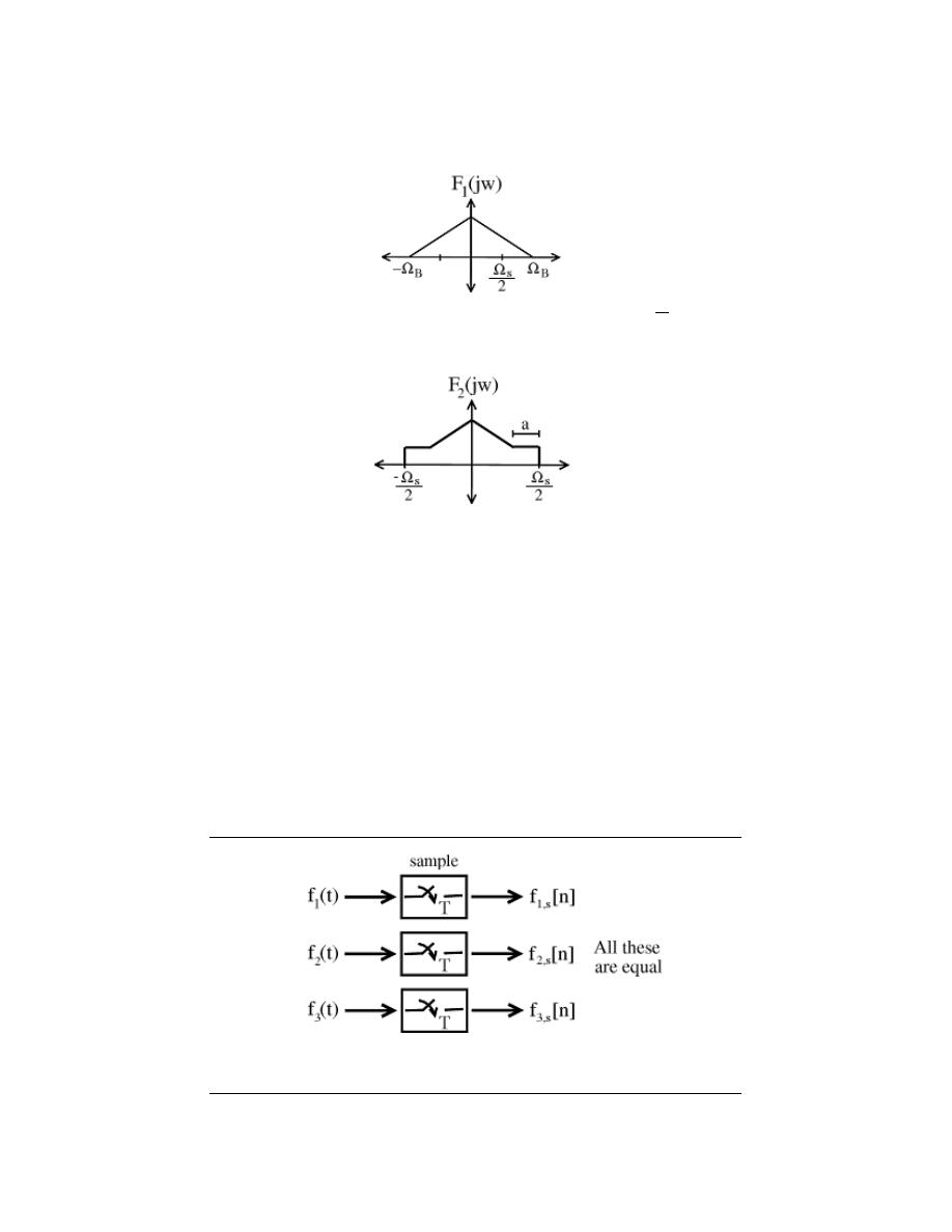
225
Figure 10.20:
In the above figure, note the following equation: Ω
B
−
Ω
s
2
= a
Figure 10.21:
The horizontal portions of the signal result from overlap with shifted
replicas - showing visual proof of aliasing.
•- What does the DTFT of f
1,s
[n] = f
1
(nT ) look like?
•- What does the DTFT of f
2,s
[n] = f
2
(nT ) look like?
•- Do any other signals have the same DTFT as f
1,s
[n] and f
2,s
[n]?
CONCLUSION: If we sample below the Nyquist frequency, there are many signals that
could have produced that given sample sequence.
Why the term ”aliasing”? Because the same sample sequence can represent different
CT signals (as opposed to when we sample above the Nyquist frequency, then the sample
sequence represents a unique CT signal).
Example 10.5:
Figure 10.22:
These are all equal!
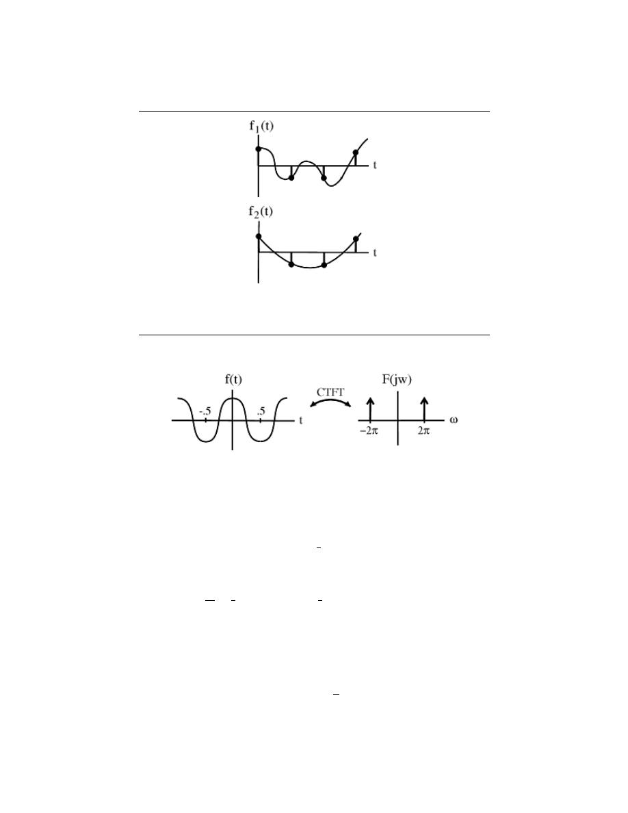
226
CHAPTER 10. SAMPLING THEOREM
Figure 10.23:
These two signals contain the same four samples, yet are very different
signals.
Figure 10.24:
The figure shows the cosine function, f (t) = cos (2πt), and its CTFT.
f (t) = cos (2πt)
Case 1: Sample Ω
s
= 8π rad/sec ⇒ T =
1
4
sec.
note:
Ω
s
> 2Ω
B
Case 2: Sample
w
Ω
s
=
8
3
π rad/sec ⇒ T =
3
4
sec
note:
Ω
s
< 2Ω
B
When we run the DTFT from Case #2 through the reconstruction steps, we realize
that we end up with the following cosine:
˜
f (t) = cos
π
2
t
This is a ”stretched” out version of our original. Clearly, our sampling rate was
not high enough to ensure correct reconstruction from the samples.
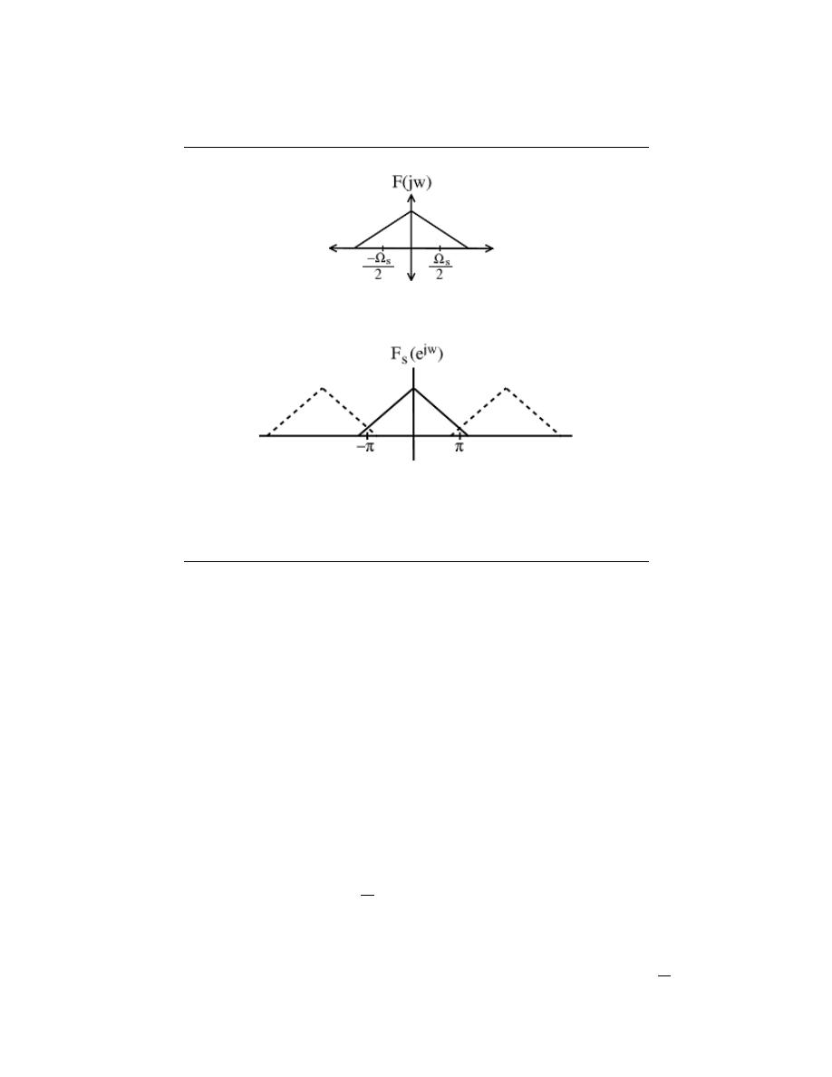
227
(a)
(b)
Figure 10.25:
(a) (b)
11.6 Anti-Aliasing Filters
10.6.1 Introduction
The idea of aliasing has been described as the problem that occurs if a signal is not sampled
at a high enough rate (for example, below the Nyquist Frequency). But exactly what kind
of distortion does aliasing produce?
High frequencies in the original signal ”fold back” into lower frequencies
High frequencies masquerading as lower frequencies produces highly undesirable artifacts
in the reconstructe signal.
warning:
We must avoid aliasing anyway we can
10.6.2 Avoiding Aliasing
What if it is impractical/impossible to sample at Ω
s
> 2Ω
B
?
Filter out the frequencies above
Ω
s
2
before you sample. The best way to visualize doing
this is to imagine the following simple steps:
1. - Take the CTFT of the signal, f (t).
2. - Send this signal through a lowpass filter with the following specification, ω
c
=
Ω
s
2
.
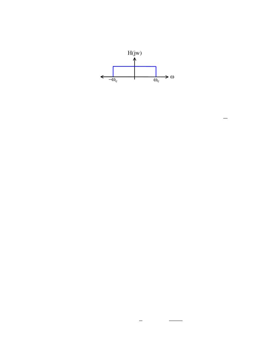
228
CHAPTER 10. SAMPLING THEOREM
Figure 10.26:
This filter will cutoff the higher, unnecessary frequencies, where |ω
c
| >
2π22kHz
3. - We now have a graph of our signal in the frequency domain with all values of |ω| >
Ω
s
2
equal to zero. Now, we take the inverse CTFT to get back our continuous time signal,
f
a
(t).
4. - And finally we are ready to sample our signal!
Example 10.6:
Sample rate for CD = 44.1 KHz
Many musical instruments (e.g. highhat) contain frequencies above 22 KHz (even
though we cannot hear them)
Because of this, we can filter the output signal from the instrument before we
sample it using the following filter:
Now the signal is ready to be sampled!
Example 10.7:
Another Example
Speech bandwidth is > ±20 KHz, but it is perfectly intelligible when lowpass
filtered to a ±4 kHz range. Because of this, we can take a normal speech signal
and pass it through a filter like the one shown in Figure 10.26, where we now set
|ω
c
| > 2π4kHz. The signal we receive from this filter only contains values where
|ω| > 8πk.
Now we can sample at 16πk = 8 KHz – standard telephony rate.
11.7 Discrete Time Processing of Continuous TIme Sig-
nals
How is the CTFT of y(t) related to the CTFT of F(t)?
Let G (jω) = reconstruction filter freq. response
Y (jω) = G (jω) Y
imp
(jω)
where Y
imp
(jω) is impulse sequence created from y
s
[n]. So,
Y (jω) = G (jω) Y
s
e
jωT
= G (jω) H e
jωT
F
s
e
jωT
Y (jω) = G (jω) H e
jωT
1
T
∞
X
r=−∞
F
j
ωF 2πr
T
!
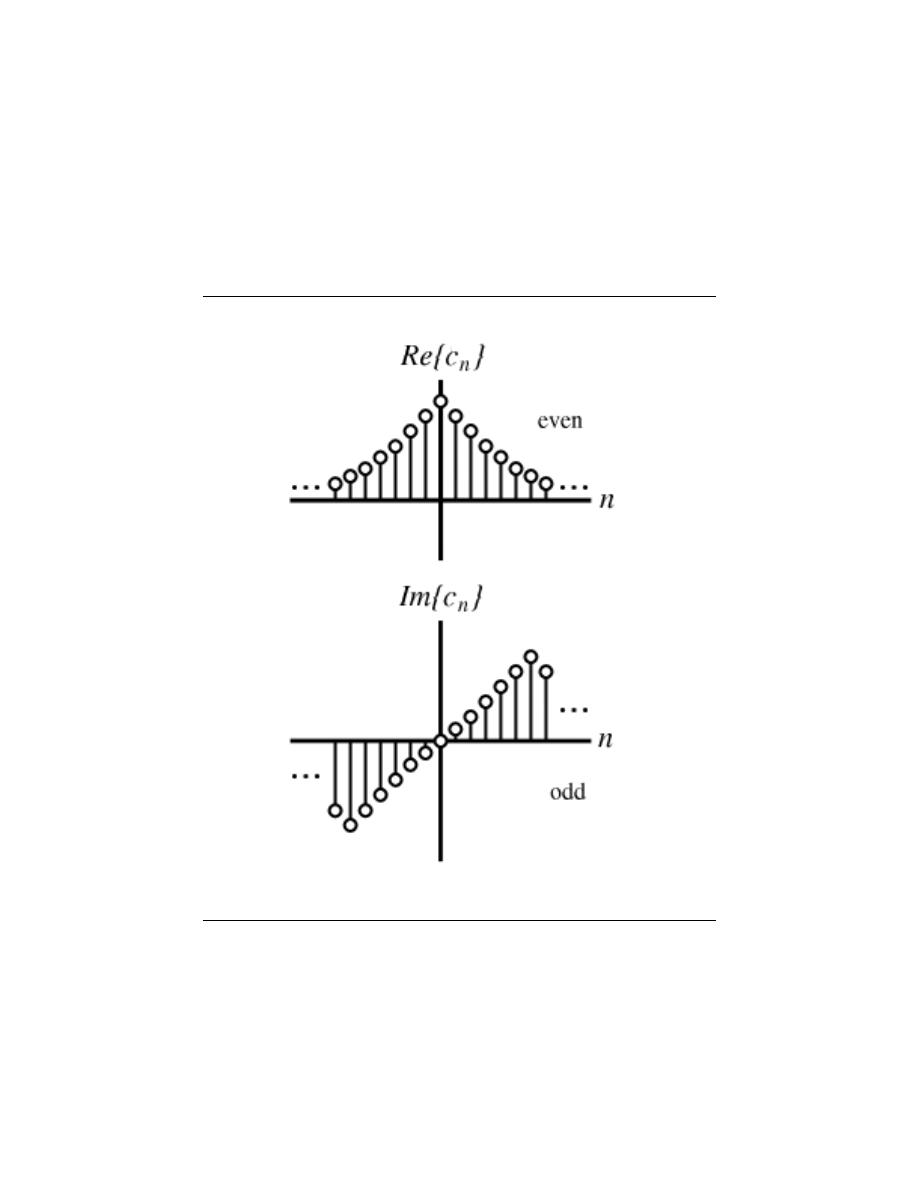
229
Figure 10.27:
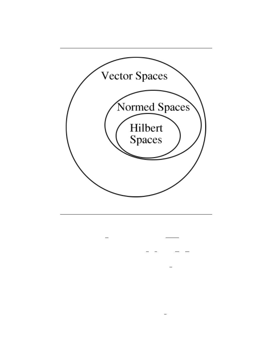
230
CHAPTER 10. SAMPLING THEOREM
Figure 10.28:
Y (jω) =
1
T
G (jω) H e
jωT
∞
X
r=−∞
F
j
ωF 2πr
T
Now, lets assume that f(t) is bandlimited to
−
π
T
,
π
T
= −
Ω
s
2
,
Ω
s
2
and G (jω) is a
perfect reconstruction filter. Then
Y (jω) =
F (jω) H e
jωT
if |ω| ≤
π
T
0 otherwise
note:
Y (jω) has the same ”bandlimit” as F (jω).
So, for bandlimited signals, and with a high enough sampling rate and a perfect reconstruc-
tion filter
is equivalent to using an analog LTI filter
where
H
a
(jω) =
H e
jωT
if |ω| ≤
π
T
0 otherwise
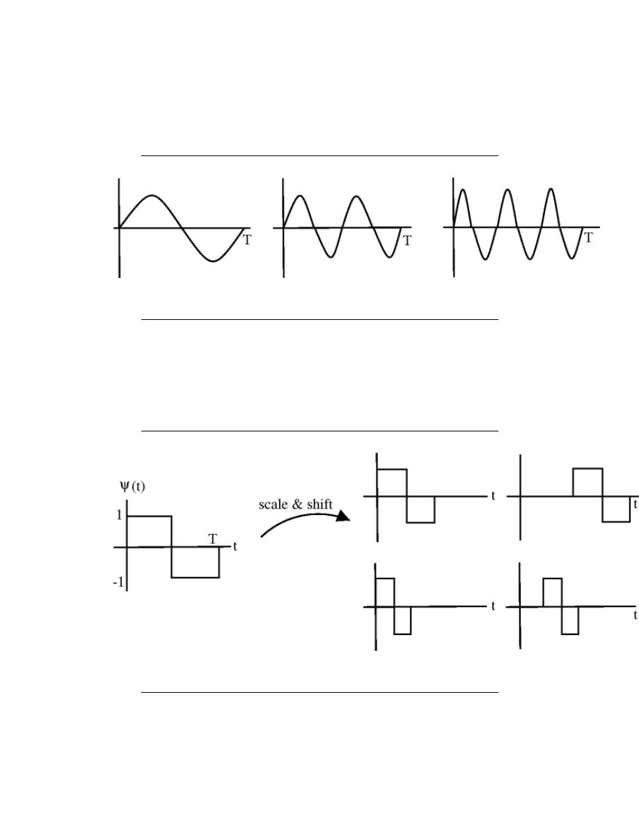
231
Figure 10.29:
Figure 10.30:

232
CHAPTER 10. SAMPLING THEOREM
So, by being careful we can implement LTI systems for bandlimited signals on our com-
puter!!!
Important note:
H
a
(jω) = filter induced by our system.
H
a
(jω) is LTI only if
• - h, the DT system, is LTI
• - F (jω), the input, is bandlimited and the sample rate is high enough.

233
Figure 10.31:

234
CHAPTER 10. SAMPLING THEOREM

Chapter 11
Laplace Transform and System
Design
12.1 The Laplace Transforms
The Laplace transform is a generalization of the Continuous-Time Fourier Transform. How-
ever, instead of using complex sinusoids of the form e
jωt
, as the CTFT does, the Laplace
transform uses the more general, e
st
, where s = σ + jω.
Although Laplace transforms are rarely solved using integration (tables and computers
(eg Matlab) are much more common), we will provide the bilateral Laplace transform
pair here. These define the forward and inverse Laplace transformations. Notice the simi-
larities between the forward and inverse transforms. This will give rise to many of the same
symmetries found in Fourier analysis.
Laplace Transform
F (s) =
Z
∞
−∞
f (t) e
−(st)
dt
(11.1)
Inverse Laplace Transform
f (t) =
1
2πj
Z
c+j∞
c−j∞
F (s) e
st
ds
(11.2)
11.1.1 Finding the Laplace and Inverse Laplace Transforms
11.1.1.1 Solving the Integral
Probably the most difficult and least used method for finding the Laplace transform of
a signal is solving the integral. Although it is technically possible, it is extremely time
consuming. Given how easy the next two methods are for finding it, we will not provide
any more than this. The integrals are primarily there in order to understand where the
following methods originate from.
11.1.1.2 Using a Computer
Using a computer to find Laplace transforms is relatively painless. Matlab has two functions,
laplace and ilaplace, that are both part of the symbolic toolbox, and will find the Laplace
235

236
CHAPTER 11. LAPLACE TRANSFORM AND SYSTEM DESIGN
and inverse Laplace transforms respectively. This method is generally preferred for more
complicated functions. Simpler and more contrived functions are usually found easily enough
by using tables (Section 11.1.1.3).
11.1.1.3 Using Tables
When first learning about the Laplace transform, tables are the most common means for
finding it. With enough practice, the tables themselves may become unnecessary, as the
common transforms can become second nature. For the purpose of this section, we will focus
on the inverse Laplace transform, since most design applications will begin in the Laplace
domain and give rise to a result in the time domain. The method is as follows:
1. - Write the function you wish to transform, H (s), as a sum of other functions, H (s) =
P
m
i=1
(H
i
(s)) where each of the H
i
is known from a table.
2. - Invert each H
i
(s) to get its h
i
(t).
3. - Sum up the h
i
(t) to get h (t) =
P
m
i=1
(h
i
(t))
Example 11.1:
Compute h (t) for ∀s, Re (s) > −5 : H (s) =
1
s+5
This can be solved directly from the table to be h (t) = e
−(5t)
Example 11.2:
Find the time domain representation, h (t), of ∀s, Re (s) > −10 : H (s) =
25
s+10
To solve this, we first notice that H (s) can also be written as 25
1
s+10
. We can
then go to the table to find h (t) = 25e
−(10t)
Example 11.3:
We can now extend the two previous examples by finding h (t) for ∀s, Re (s) > −5 :
H (s) =
1
s+5
+
25
s+10
To do this, we take advantage of the additive property of linearity and the three-
step method described above to yield the result h (t) = e
−(5t)
+ 25e
−(10t)
For more complicated examples, it may be more difficult to break up the transfer function
into parts that exist in a table. In this case, it is often necessary to use partial fraction
expansion to get the transfer function into a more usable form.
11.1.2 Visualizing the Laplace Transform
With the Fourier transform, we had a complex-valued function of a purely imaginary
variable, F (jω). This was something we could envision with two 2-dimensional plots (real
and imaginary parts or magnitude and phase). However, with Laplace, we have a complex-
valued function of a complex variable. In order to examine the magnitude and phase or
real and imaginary parts of this function, we must examine 3-dimensional surface plots of
each component.
While these are legitimate ways of looking at a signal in the Laplace domain, it is quite
difficult to draw and/or analyze. For this reason, a simpler method has been developed.
Although it will not be discussed in detail here, the method of Poles and Zeros is much easier
to understand and is the way both the Laplace transform and its discrete-time counterpart
the Z-transform are represented graphically.
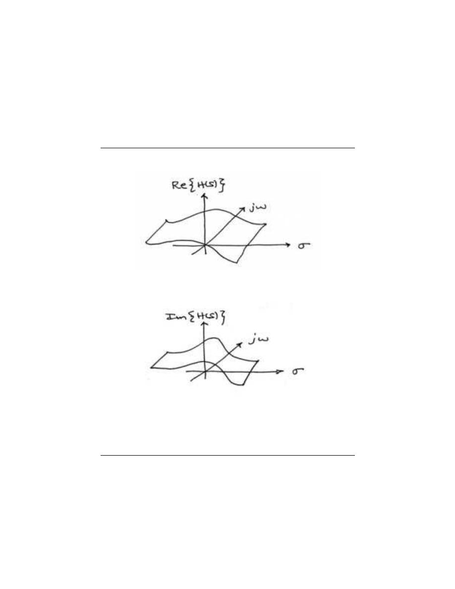
237
real and imaginary sample plots
(a)
(b)
Figure 11.1:
Real and imaginary parts of H (s) are now each 3-dimensional surfaces.
(a) The Real part of H (s) (b) The Imaginary part of H (s)
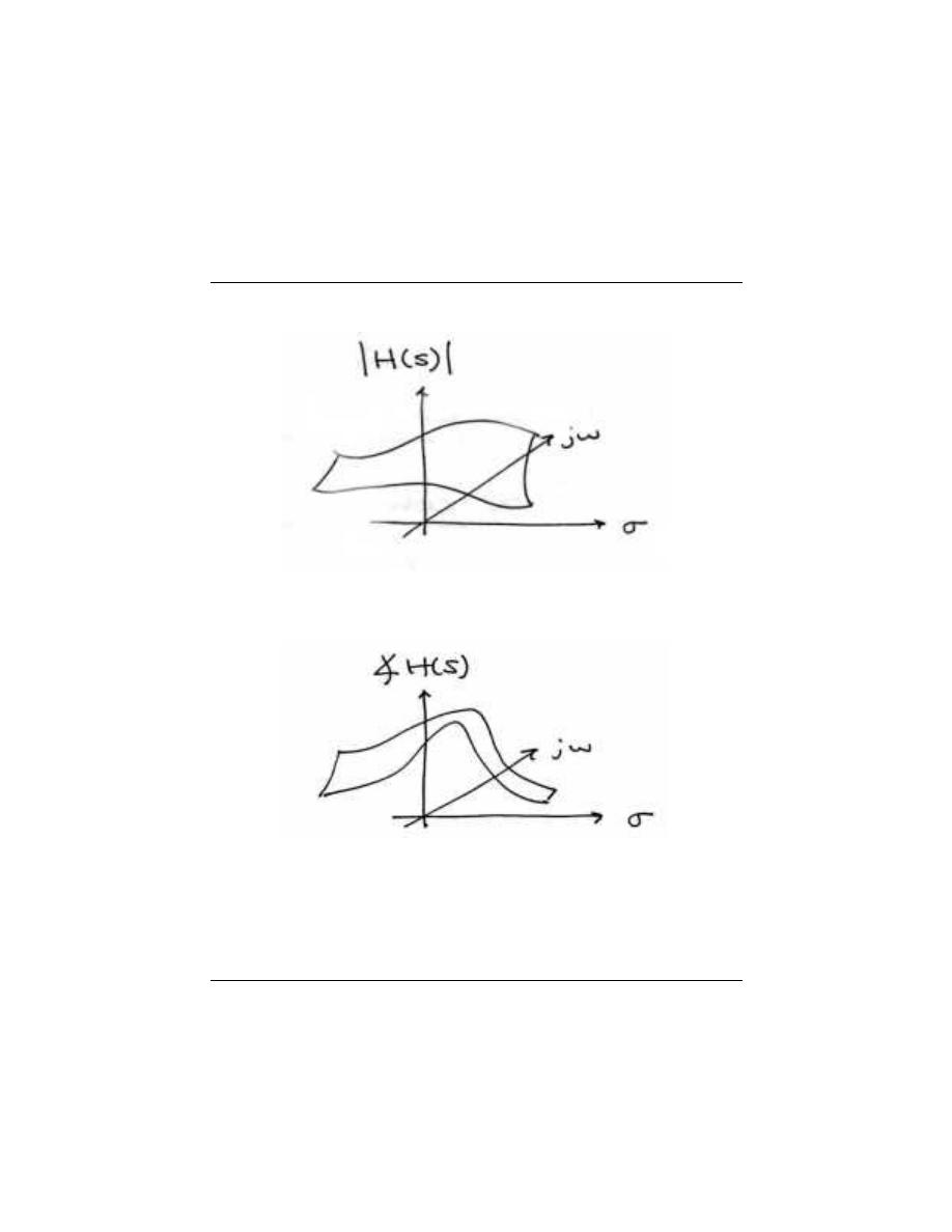
238
CHAPTER 11. LAPLACE TRANSFORM AND SYSTEM DESIGN
magnitude and phase sample plots
(a)
(b)
Figure 11.2:
Magnitude and phase of H (s) are also each 3-dimensional surfaces. This
representation is more common than real and imaginary parts. (a) The Magnitude of
H (s) (b) The Phase of H (s)

239
12.2 Properties of the Laplace Transform
Property
Signal
Laplace Transform
Region of Conver-
gence
Linearity
αx
1
(t) + βx
2
(t)
αX
1
(s) + βX
2
(s)
At
least
ROC
1
T ROC
2
Time Shifting
x (t − τ )
e
−(sτ )
X (s)
ROC
Frequency
Shifting
(modulation)
e
ηt
x (t)
X (s − η)
Shifted ROC ( s − η
must be in the region
of convergence)
Time Scaling
x (αt)
(1 − |α|) X (s − α)
Scaled ROC ( s − α
must be in the region
of convergence)
Conjugation
x (t)
∗
X (s
∗
)
∗
ROC
Convolution
x
1
(t) ∗ x
2
(t)
X
1
(t) X
2
(t)
At
least
ROC
1
T ROC
2
Time Differentiation
d
dt
x (t)
sX (s)
At least ROC
Frequency Differen-
tiation
(−t) x (t)
d
ds
X (s)
ROC
Integration in Time
R
t
−∞
x (τ ) dτ
(1 − s) X (s)
At
least
ROC
T Re (s) > 0
12.3 Table of Common Laplace Transforms
Signal
Laplace Transform
Region of Convergence
δ (t)
1
All s
δ (t − T )
e
−(sT )
All s
u (t)
1
s
Re (s) > 0
− (u (−t))
1
s
Re (s) < 0
tu (t)
1
s
2
Re (s) > 0
t
n
u (t)
n!
s
n+1
Re (s) > 0
− (t
n
u (−t))
n!
s
n+1
Re (s) < 0
e
−(λt)
u (t)
1
s+λ
Re (s) > −λ
− e
−(λt)
u (−t)
1
s+λ
Re (s) < −λ
te
−(λt)
u (t)
1
(s−λ)
2
Re (s) > −λ
t
n
e
−(λt)
u (t)
n!
(s+λ)
n+1
Re (s) > −λ
− t
n
e
−(λt)
u (−t)
n!
(s+λ)
n+1
Re (s) < −λ
cos (bt) u (t)
s
s
2
+b
2
Re (s) > 0
sin (bt) u (t)
b
s
2
+b
2
Re (s) > 0
e
−(at)
cos (bt) u (t)
s+a
(s+a)
2
+b
2
Re (s) > −a
e
−(at)
sin (bt) u (t)
b
(s+a)
2
+b
2
Re (s) > −a
d
n
dt
n
δ (t)
s
n
All s

240
CHAPTER 11. LAPLACE TRANSFORM AND SYSTEM DESIGN
12.4 Region of Convergence for the Laplace Transform
With the Laplace transform, the s-plane represents a set of signals (complex exponentials).
For any given LTI system, some of these signals may cause the output of the system to
converge, while others cause the output to diverge (”blow up”). The set of signals that
cause the system’s output to converge lie in the region of convergence (ROC) . This
module will discuss how to find this region of convergence for any continuous-time, LTI
system.
Recall the definition of the Laplace transform,
Laplace Transform
H (s) =
Z
∞
−∞
h (t) e
−(st)
dt
(11.3)
If we consider a causal, complex exponential, h (t) = e
−(at)
u (t), we get the equation,
Z
∞
0
e
−(at)
e
−(st)
dt =
Z
∞
0
e
−((a+s)t)
dt
(11.4)
Evaluating this, we get
−1
s + a
lim
t→∞
e
−((s+a)t)
− 1
(11.5)
Notice that this equation will tend to infinity when lim
t→∞
e
−((s+a)t)
tends to infinity. To
understand when this happens, we take one more step by using s = σ + jω to realize this
equation as
lim
t→∞
e
−(jωt)
e
−((σ+a)t)
(11.6)
Recognizing that e
−(jωt)
is sinusoidal, it becomes apparent that e
−(σ(a)t)
is going to deter-
mine whether this blows up or not. What we find is that if σ + a is positive, the exponential
will be to a negative power, which will cause it to go to zero as t tends to infinity. On the
other hand, if σ + a is negative or zero, the exponential will not be to a negative power,
which will prevent it from tending to zero and the system will not converge. What all of
this tells us is that for a causal signal, we have convergence when
Condition for Convergence
Re (s) > −a
(11.7)
Although we will not go through the process again for anticausal signals, we could. In
doing so, we would find that the necessary condition for convergence is when
Necessary Condition for Anti-Causal Convergence
Re (s) < −a
(11.8)
11.4.1 Graphical Understanding of ROC
Perhaps the best way to look at the region of convergence is to view it in the s-plane. What
we observe is that for a single pole, the region of convergence lies to the right of it for causal
signals and to the left for anti-causal signals.
Once we have recognized this, the natural question becomes: What do we do when we
have multiple poles? The simple answer is that we take the intersection of all of the regions
of convergence of the respective poles.
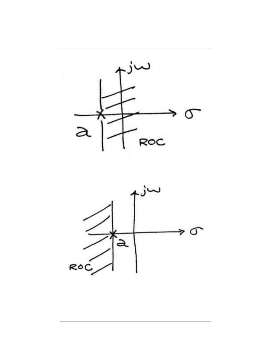
241
(a)
(b)
Figure 11.3:
(a) The Region of Convergence for a causal signal. (b) The Region of
Convergence for an anti-causal signal.
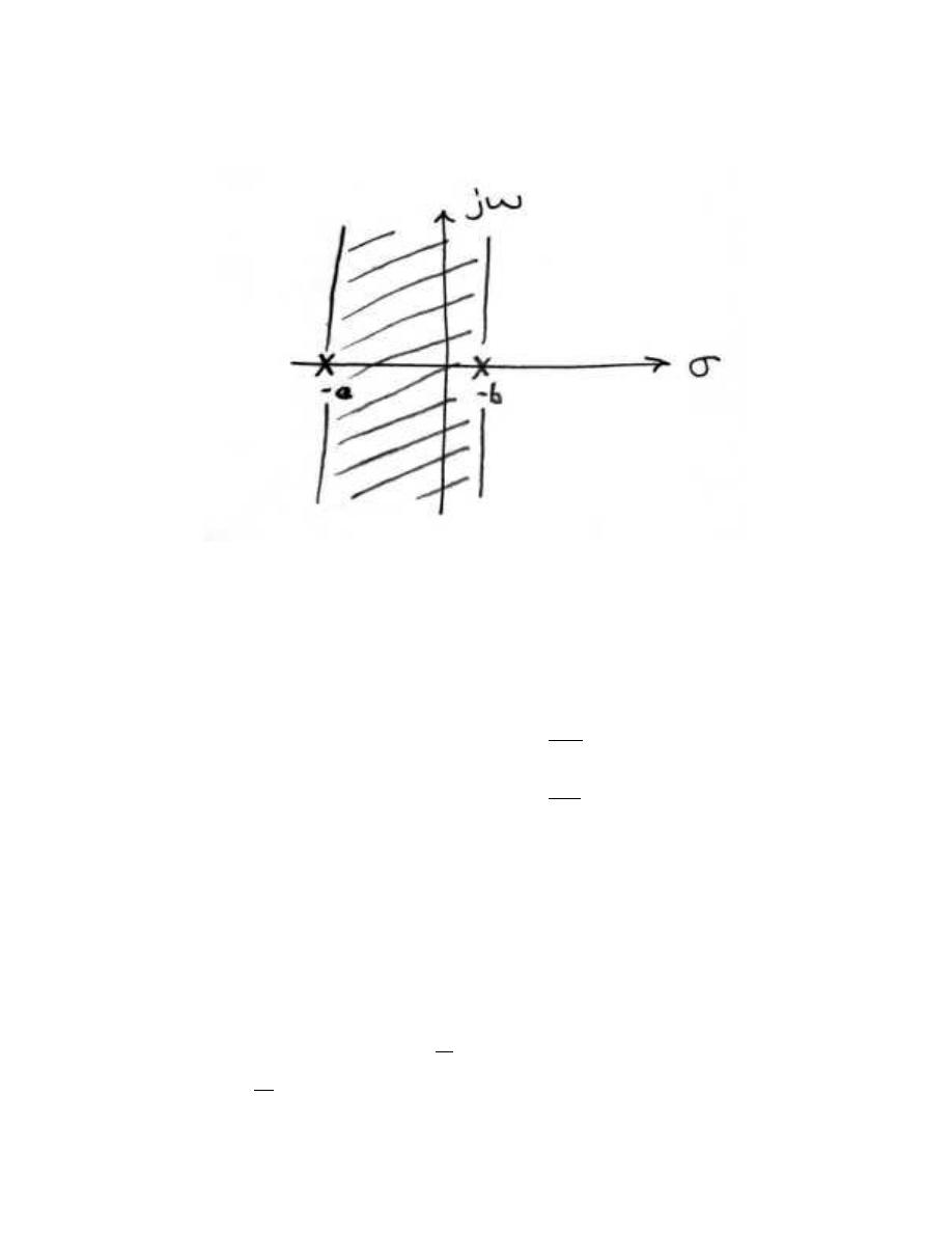
242
CHAPTER 11. LAPLACE TRANSFORM AND SYSTEM DESIGN
Figure 11.4: The Region of Convergence of h (t) if a > b.
Example 11.4:
Find H (s) and state the region of convergence for h (t) = e
−(at)
u (t) + e
−(bt)
u (−t)
Breaking this up into its two terms, we get transfer functions and respective regions
of convergence of
∀s, Re (s) > −a : H
1
(s) =
1
s + a
(11.9)
and
∀s, Re (s) < −b : H
2
(s) =
−1
s + b
(11.10)
Combining these, we get a region of convergence of −b > Re (s) > −a. If a > b, we
can represent this graphically. Otherwise, there will be no region of convergence.
12.5 The Inverse Laplace Transform
11.5.1 To Come
In The Transfer Function(FIX ME TO CHAPTER 9.2) we shall establish that the inverse
Laplace transform of a function h is
@@@
−1
(h)
(t) =
1
2π
Z
∞
−∞
e
(c+yj)t
h ((c + yj) t) dy,
(11.11)
where j ≡
√
−1 and the real number c is chosen so that all of the singularities of h lie to
the left of the line of integration.

243
11.5.2 Proceeding with the Inverse Laplace Transform
With the inverse Laplace transform one may express the solution of x
0
= Bx + g , as
x (t) = @@@
−1
(sI − B)
−1
(@@@g + x (0)) .
(11.12)
As an example, let us take the first component of @@@x, namely
@@@
x
1
(s) =
0.19 s
2
+ 1.5s + 0.27
s +
1
6
4
(s
3
+ 1.655s
2
+ 0.4078s + 0.0039)
.
We define:
poles :
Also called singularities, these are the points s at which @@@
x
1
(s) blows
up.
These are clearly the roots of its denominator, namely
−1/100,@@@@@@@@@@@@@@@@@@
−329/400 ±
√
73
16
!
,@@@@@@@@@@@@@@@@@@and@@@@@@@@@@@@@@@@@@−1/6.
(11.13)
All four being negative, it suffices to take c = 0 and so the integration in Equation 11.11
proceeds up the imaginary axis. We don’t suppose the reader to have already encountered
integration in the complex plane but hope that this example might provide the motivation
necessary for a brief overview of such. Before that however we note that MATLAB has
digested the calculus we wish to develop. Referring again to fib3.m
1
for details we note that
the ilaplace command produces
x
1
(t) = 211.35e
−t
100
− 0.0554t
3
+ 4.5464t
2
+ 1.085t + 474.19
e
−t
6
+e
−(329t)
400
262.842cosh
√
73t
16
!!
+262.836sinh
√
73t
16
!
The other potentials, see the figure above, possess similar expressions. Please note that
each of the poles of @@@x
1
appear as exponents in x
1
and that the coefficients of the
exponentials are polynomials whose degrees is determined by the order of the respective
pole.
12.6 Poles and Zeros
11.6.1 Introduction
It is quite difficult to qualitatively analyze the Laplace transform and Z-transform, since
mappings of their magnitude and phase or real part and imaginary part result in multiple
mappings of 2-dimensional surfaces in 3-dimensional space. For this reason, it is very com-
mon to examine a plot of a transfer function’s poles and zeros to try to gain a qualitative
idea of what a system does.
Given a continuous-time transfer function in the Laplace domain, H (s), or a discrete-
time one in the Z-domain, H (z), a zero is any value of s or z such that the transfer function
is zero, and a pole is any value of s or z such that the transfer function is infinite. To define
them precisely:
1
http://www.caam.rice.edu/∼caam335/cox/lectures/fib3.m
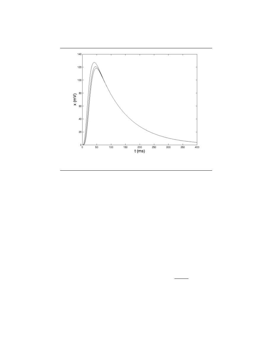
244
CHAPTER 11. LAPLACE TRANSFORM AND SYSTEM DESIGN
Figure 11.5:
The 3 potentials associated with the RC circuit model figure (pg ??).
zeros :
1. The value(s) for z where the numerator of the transfer function equals zero
2. The complex frequencies that make the overall gain of the filter transfer function
zero.
poles :
1. The value(s) for z where the denominator of the transfer function equals zero
2. The complex frequencies that make the overall gain of the filter transfer function
infinite.
11.6.2 Pole/Zero Plots
When we plot these in the appropriate s- or z-plane, we represent zeros with ”o” and poles
with ”x”. Refer to this module for a detailed looking at plotting the poles and zeros of a
z-transform on the Z-plane.
Example 11.5:
Find the poles and zeros for the transfer function H (s) =
s
2
+6s+8
s
2
+2
and plot the
results in the s-plane.
The first thing we recognize is that this transfer function will equal zero whenever
the top, s
2
+ 6s + 8, equals zero. To find where this equals zero, we factor this to
get, (s + 2) (s + 4). This yields zeros at s = −2 and s = −4. Had this function
been more complicated, it might have been necessary to use the quadratic formula.
For poles, we must recognize that the transfer function will be infinite whenever
the bottom part is zero. That is when s
2
+ 2 is zero. To find this, we again look to
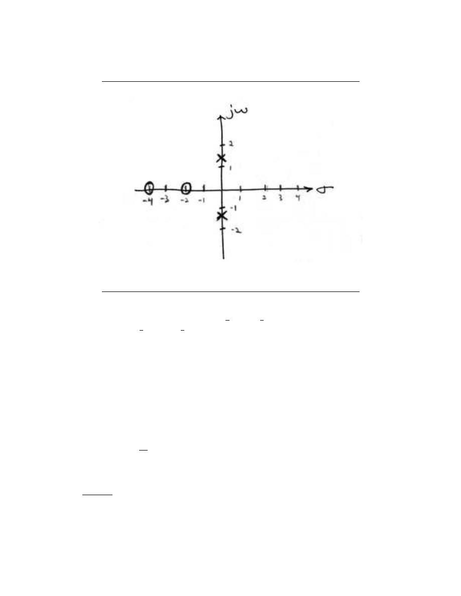
245
Pole and Zero Plot
Figure 11.6: Sample pole-zero plot
factor the equation. This yields s + j
√
2
s − j
√
2
. This yields purely imaginary
roots of +j
√
2 and − j
√
2
Plotting this gives
Now that we have found and plotted the poles and zeros, we must ask what it is that
this plot gives us. Basically what we can gather from this is that the magnitude of the
transfer function will be larger when it is closer to the poles and smaller when it is closer
to the zeros. This provides us with a qualitative understanding of what the system does at
various frequencies and is crucial to the discussion of stability.
11.6.3 Repeated Poles and Zeros
It is possible to have more than one pole or zero at any given point. For instance, the discrete-
time transfer function H (z) = z
2
will have two zeros at the origin and the continuous-time
function H (s) =
1
s
25
will have 25 poles at the origin.
11.6.4 Pole-Zero Cancellation
An easy mistake to make with regards to poles and zeros is to think that a function like
(s+3)(s−1)
s−1
is the same as s + 3. In theory they are equivalent, as the pole and zero at s = 1
cancel each other out in what is known as pole-zero cancellation . However, think about
what may happen if this were a transfer function of a system that was created with physical
circuits. In this case, it is very unlikely that the pole and zero would remain in exactly the
same place. A minor temperature change, for instance, could cause one of them to move
just slightly. If this were to occur a tremendous amount of volatility is created in that area,

246
CHAPTER 11. LAPLACE TRANSFORM AND SYSTEM DESIGN
since there is a change from infinity at the pole to zero at the zero in a very small range of
signals. This is generally a very bad way to try to eliminate a pole. A much better way is
to use control theory to move the pole to a better place.

Chapter 12
Z-Transform and Digital
Filtering
13.1 The Z Transform: Definition
12.1.1 Basic Definition of the Z-Transform
The z-transform of a sequence is defined as
X (z) =
∞
X
n=−∞
x [n] z
−n
(12.1)
Sometimes this equation is referred to as the bilateral z-transform . At times the z-
transform is defined as
X (z) =
∞
X
n=0
x [n] z
−n
(12.2)
which is known as the unilateral z-transform .
There is a close relationship between the z-transform and the Fourier transform of a
discrete time signal, which is defined as
X e
jω
=
∞
X
n=−∞
x [n] e
−(jωn)
(12.3)
Notice that that when the z
−n
is replaced with e
−(jωn)
the z-transform reduces to the
Fourier Transform. When the Fourier Transform exists, z = e
jω
, which is to have the
magnitude of z equal to unity.
12.1.2 The Complex Plane
In order to get further insight into the relationship between the Fourier Transform and the
Z-Transform it is useful to look at the complex plane or z-plane . Take a look at the
complex plane:
The Z-plane is a complex plane with an imaginary and real axis referring to the complex-
valued variable z. The position on the complex plane is given by re
jω
, and the angle from
the positive, real axis around the plane is denoted by ω. X (z) is defined everywhere on this
plane. X e
jω
on the other hand is defined only where |z| = 1, which is refered to as the
247
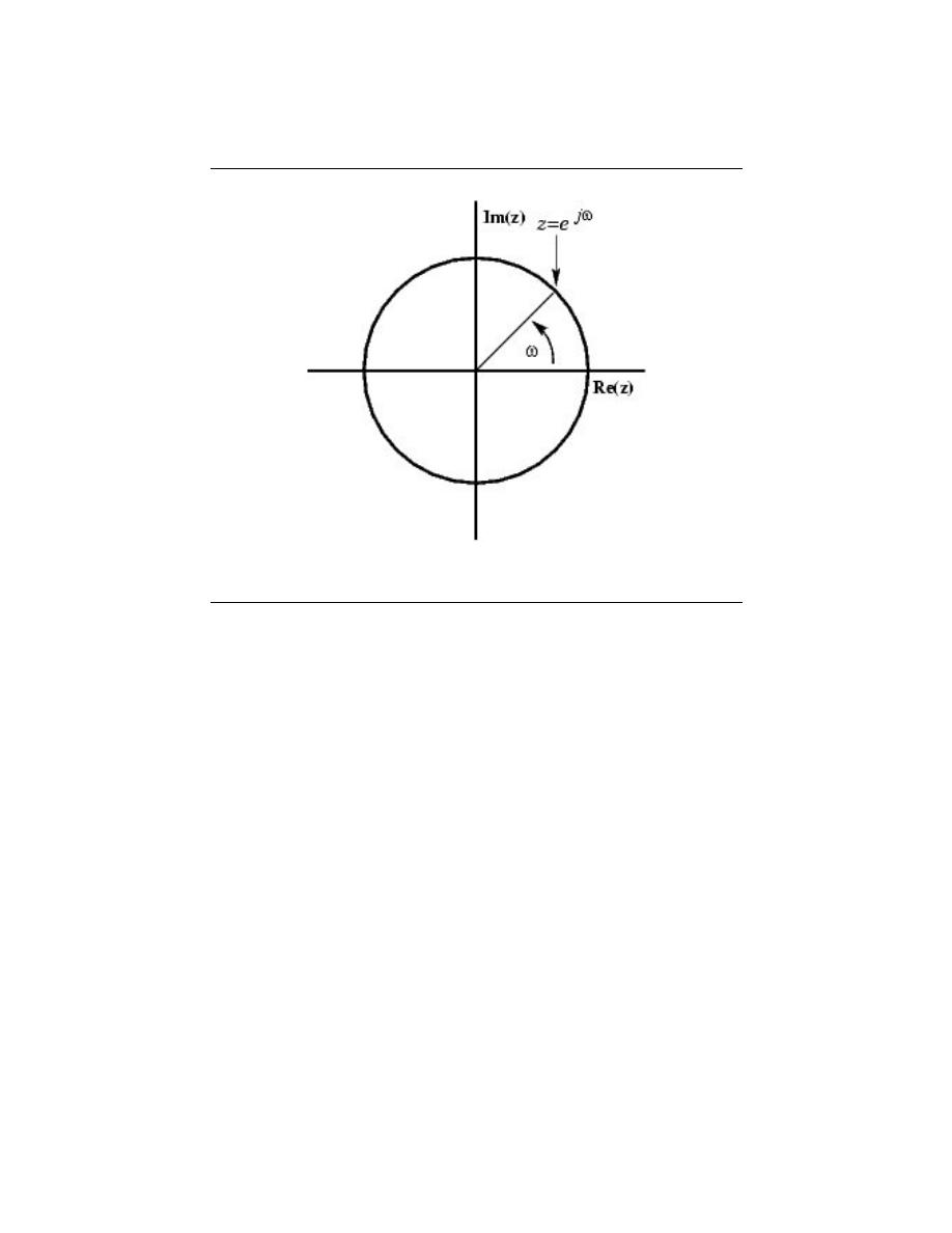
248
CHAPTER 12. Z-TRANSFORM AND DIGITAL FILTERING
Z-Plane
Figure 12.1
unit circle. So for example, ω = 1 at z = 1 and ω = π at z = −1. This is usefull because,
by representing the Fourier transform as the z-transform on the unit circle, the periodicity
of Fourier transform is easily seen.
12.1.3 Region of Convergence
The region of convergence, known as the ROC , is important to understand because it
defines the region where the z-transform exists. The ROC for a given x [n] , is defined as
the range of z for which the z-transform converges. Since the z-transform is a power series
, it converges when x [n] z
−n
is absolutely summable. Stated differently,
∞
X
n=−∞
|x [n] z
−n
|
< ∞
(12.4)
must be satisfied for convergence. This is best illustrated by looking at the different ROC’s
of the z-transforms of α
n
u [n] and α
n
u [n − 1] .
Example 12.1:
For
x [n] = α
n
u [n]
(12.5)
X (z)
=
P
∞
n=−∞
(x [n] z
−n
)
=
P
∞
n=−∞
(α
n
u [n] z
−n
)
=
P
∞
n=0
(α
n
z
−n
)
=
P
∞
n=0
αz
−1
n
(12.6)
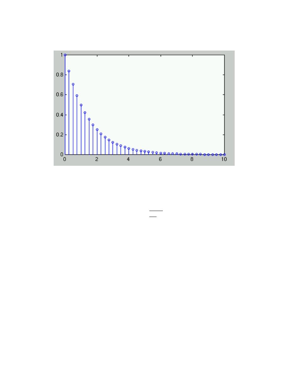
249
Figure 12.2:
x [n] = α
n
u [n] where α = .5.
This sequence is an example of a right-sided exponential sequence because it is
nonzero for n ≥ 0. It only converges when |αz
−1
| < 1. When it converges,
X (z)
=
1
1−αz
−1
=
z
z−α
(12.7)
If |αz
−1
| ≥ 1, then the series,
P
∞
n=0
αz
−1
n
does not converge. Thus the ROC
is the range of values where
|αz
−1
| < 1
(12.8)
or, equivalently,
|z| > |α|
(12.9)
Example 12.2:
For
x [n] = (− (α
n
)) u [−n − 1]
(12.10)
X (z)
=
P
∞
n=−∞
(x [n] z
−n
)
=
P
∞
n=−∞
((− (α
n
)) u [−n − 1] z
−n
)
=
−
P
−1
n=−∞
(α
n
z
−n
)
=
−
P
−1
n=−∞
α
−1
z
−n
=
−
P
∞
n=1
α
−1
z
n
=
1 −
P
∞
n=0
α
−1
z
n
(12.11)
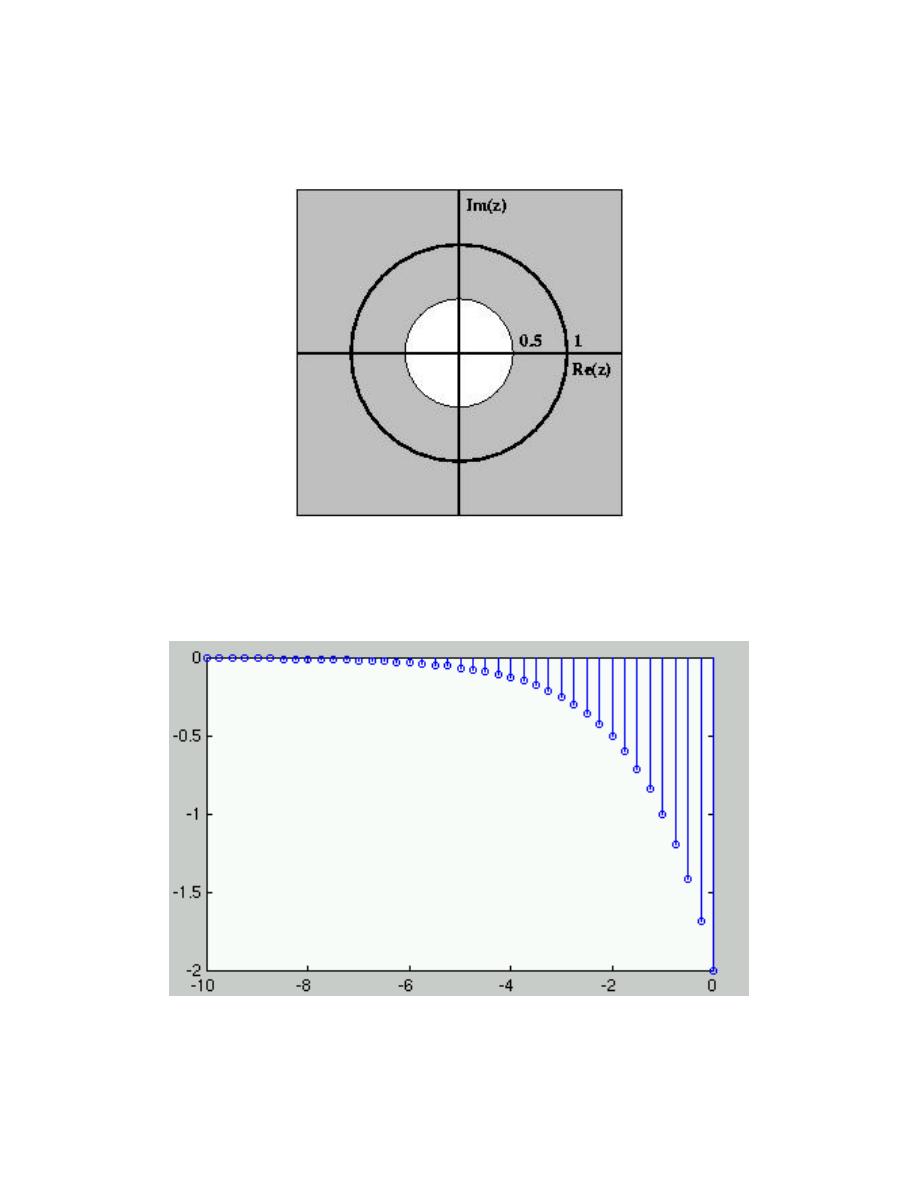
250
CHAPTER 12. Z-TRANSFORM AND DIGITAL FILTERING
Figure 12.3: ROC for x [n] = α
n
u [n] where α = 0.5
Figure 12.4:
x [n] = (− (α
n
)) u [−n − 1] where α = .5.
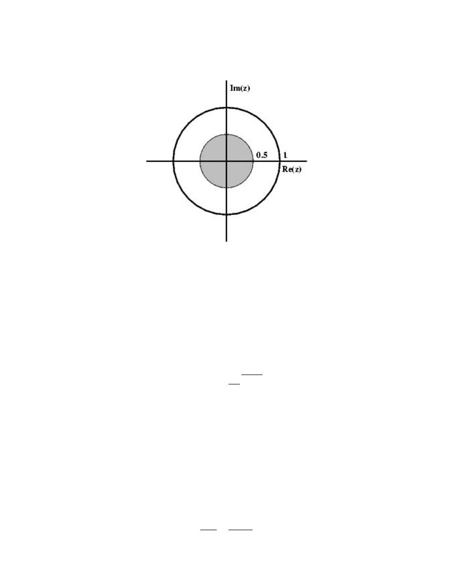
251
Figure 12.5: ROC for x [n] = (− (α
n
)) u [−n − 1]
The ROC in this case is the range of values where
|α
−1
z| < 1
(12.12)
or, equivalently,
|z| < |α|
(12.13)
If the ROC is satisfied, then
X (z)
=
1 −
1
1−α
−1
z
=
z
z−α
(12.14)
13.2 Table of Common Z-Transforms
The table below will focus on unilateral and bilateral z-transforms . When given a signal
(or sequence), the table can be very useful in finding the corresponding z-transform. The
table also specifies the region of convergence, which allows us to pick out the unilateral and
bilateral transforms.
note:
The notation for z found in the table below may differ from that found in
other tables. For example, the basic z-transform of u [n] can be written as either
of the following two expressions, which are equal:
z
z − 1
=
1
1 − z
−1
(12.15)

252
CHAPTER 12. Z-TRANSFORM AND DIGITAL FILTERING
Signal
Z-Transform
ROC
δ [n − k]
z
−k
Allz
u [n]
z
z−1
|z| > 1
− (u [−n − 1])
z
z−1
|z| < 1
nu [n]
z
(z−1)
2
|z| > 1
n
2
u [n]
z(z+1)
(z−1)
3
|z| > 1
n
3
u [n]
z
(
z
2
+4z+1
)
(z−1)
4
|z| > 1
(− (α
n
)) u [−n − 1]
z
z−α
|z| < |α|
α
n
u [n]
z
z−α
|z| > |α|
nα
n
u [n]
αz
(z−α)
2
|z| > |α|
n
2
α
n
u [n]
αz(z+α)
(z−α)
3
|z| > |α|
Q
m
k=1
(n−k+1)
α
m
m!
α
n
u [n]
z
(z−α)
m+1
γ
n
cos (αn) u [n]
z(z−γcos(α))
z
2
−(2γcos(α))z+γ
2
|z| > |α|
γ
n
sin (αn) u [n]
zγsin(α)
z
2
−(2γcos(α))z+γ
2
|z| > |α|
13.3 Region of Convergence for the Z-transform
12.3.1 The Region of Convergence
The region of convergence, known as the ROC , is important to understand because it
defines the region where the z-transform exists. The z-transform of a sequence is defined
as
X (z) =
∞
X
n=−∞
x [n] z
−n
(12.16)
The ROC for a given x [n] , is defined as the range of z for which the z-transform converges.
Since the z-transform is a power series , it converges when x [n] z
−n
is absolutely summable.
Stated differently,
∞
X
n=−∞
|x [n] z
−n
|
< ∞
(12.17)
must be satisfied for convergence.
12.3.2 Properties of the Region of Convergencec
The Region of Convergence has a number of properties that are dependent on the charac-
teristics of the signal, x [n].
• - The ROC cannot contain any poles. By definition a pole is a where X (z) is infinite.
Since X (z) must be finite for all z for convergence, there cannot be a pole in the ROC.
• - If x [n] is a finite-duration sequence, then the ROC is the entire z-plane, exept possibly
z = 0 or |z| = ∞.
A finite-duration sequence is a sequence that is nonzero in a
finite interval n
1
≤ n ≤ n
2
. As long as each value of x [n] is finite then the sequence
will be absolutely summable. When n
2
> 0 there will be a z
−1
term and thus the ROC
will not include z = 0. When n
1
< 0 then the sum will be infinite and thus the ROC
will not include |z| = ∞. On the other hand, when n
2
≤ 0 then the ROC will include
z = 0, and when n
1
≥ 0 the ROC will include |z| = ∞. With these constraints, the
only signal, then, whose ROC is the entire z-plane is x [n] = cδ [n].
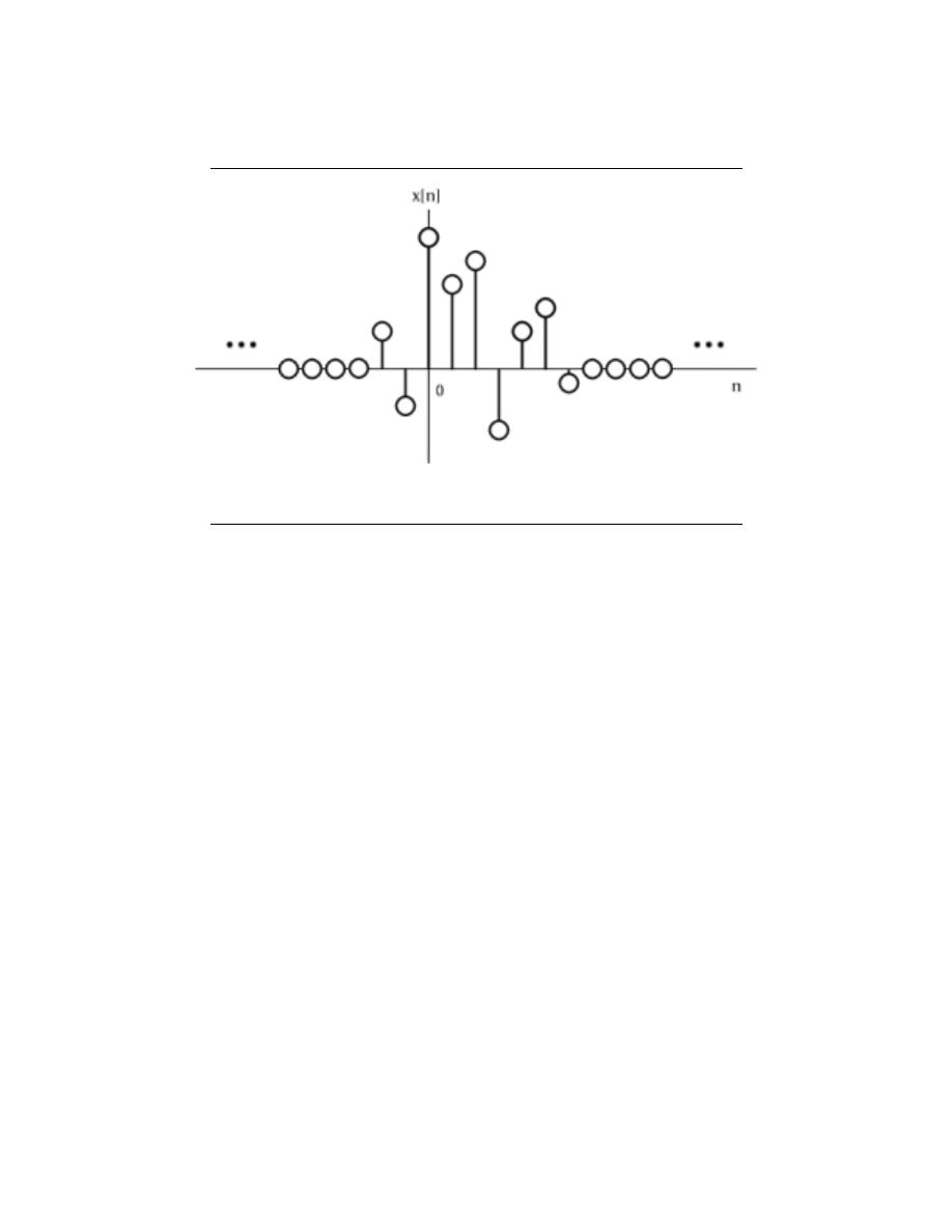
253
Figure 12.6: An example of a finite duration sequence.
The next properties apply to infinite duration sequences. As noted above, the z-transform
converges when |X (z) | < ∞. So we can write
|X (z) | = |
∞
X
n=−∞
x [n] z
−n
| ≤
∞
X
n=−∞
|x [n] z
−n
|
=
∞
X
n=−∞
|x [n] |(|z|)
−n
(12.18)
We can then split the infinite sum into positive-time and negative-time portions. So
|X (z) | ≤ N (z) + P (z)
(12.19)
where
N (z) =
−1
X
n=−∞
|x [n] |(|z|)
−n
(12.20)
and
P (z) =
∞
X
n=0
|x [n] |(|z|)
−n
(12.21)
In order for |X (z) | to be finite, |x [n] | must be bounded. Let us then set
|x (n) | ≤ C
1
r
1
n
(12.22)
for
n < 0
and
|x (n) | ≤ C
2
r
2
n
(12.23)
for
n ≥ 0
From this some further properties can be derived:
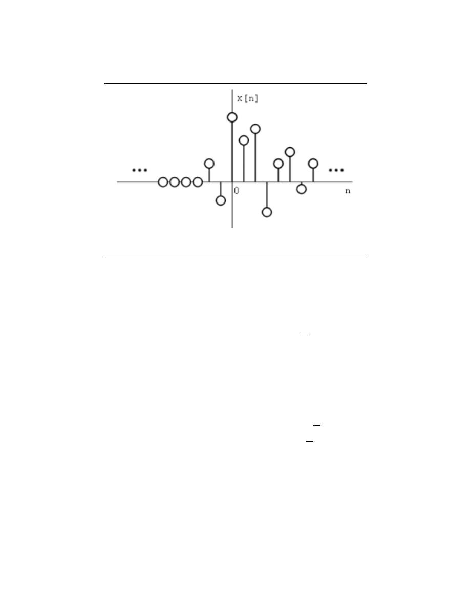
254
CHAPTER 12. Z-TRANSFORM AND DIGITAL FILTERING
Figure 12.7: A right-sided sequence.
• - If x [n] is a right-sided sequence, then the ROC extends outward from the outermost
pole in X (z). A right-sided sequence is a sequence where x [n] = 0 for n < n
1
< ∞.
Looking at the positive-time portion from the above derivation, it follows that
P (z) ≤ C
2
∞
X
n=0
r
2
n
(|z|)
−n
= C
2
∞
X
n=0
r
2
|z|
n
(12.24)
Thus in order for this sum to converge, |z| > r
2
, and therefore the ROC of a right-sided
sequence is of the form |z| > r
2
.
• - If x [n] is a left-sided sequence, then the ROC extends inward from the innermost pole
in X (z).
A right-sided sequence is a sequence where x [n] = 0 for n > n
2
> −∞.
Looking at the negative-time portion from the above derivation, it follows that
N (z) ≤
C
1
P
−1
n=−∞
r
1
n
(|z|)
−n
=
C
1
P
−1
n=−∞
r
1
|z|
n
=
C
1
P
∞
k=1
|z|
r
1
k
(12.25)
Thus in order for this sum to converge, |z| < r
1
, and therefore the ROC of a left-sided
sequence is of the form |z| < r
1
.
• - If x [n] is a two-sided sequence, the ROC will be a ring in the z-plane that is bounded
on the interior and exterior by a pole.
A two-sided sequence is an sequence with
infinite duration in the positive and negative directions. From the derivation of the
above two properties, it follows that if r
2
< |z| < r
2
converges, then both the positive-
time and negative-time portions converge and thus X (z) converges as well. Therefore
the ROC of a two-sided sequence is of the form r
2
< |z| < r
2
.
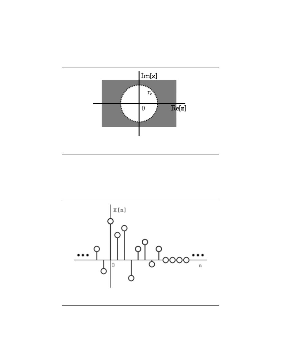
255
Figure 12.8: The ROC of a right-sided sequence.
Figure 12.9: A left-sided sequence.
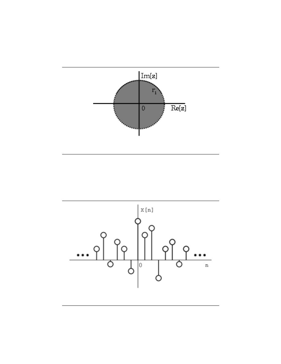
256
CHAPTER 12. Z-TRANSFORM AND DIGITAL FILTERING
Figure 12.10: The ROC of a left-sided sequence.
Figure 12.11: A two-sided sequence.

257
Figure 12.12: The ROC of a two-sided sequence.
12.3.3 Examples
To gain further insight it is good to look at a couple of examples.
Example 12.3:
Lets take
x
1
[n] =
1
2
n
u [n] +
1
4
n
u [n]
(12.26)
The z-transform of
1
2
n
u [n] is
z
z−
1
2
with an ROC at |z| >
1
2
.
The z-transform of
−1
4
n
u [n] is
z
z+
1
4
with an ROC at |z| >
−1
4
.
Due to linearity,
X
1
[z]
=
z
z−
1
2
+
z
z+
1
4
=
z
(
2z−
1
8
)
(
z−
1
2
)(
z+
1
4
)
(12.27)
By observation it is clear that there are two zeros, at 0 and
1
16
, and two poles, at
1
2
, and
−1
4
. Following the obove properties, the ROC is |z| >
1
2
.
Example 12.4:
Now take
x
2
[n] =
−1
4
n
u [n] −
1
2
n
u [−n − 1]
(12.28)
The z-transform and ROC of
−1
4
n
u [n] was shown in the example above (Exam-
ple 12.3). The z-transorm of −
1
2
n
u [−n − 1] is
z
z−
1
2
with an ROC at |z| >
1
2
.
Once again, by linearity,
X
2
[z]
=
z
z+
1
4
+
z
z−
1
2
=
z
(
2z−
1
8
)
(
z+
1
4
)(
z−
1
2
)
(12.29)
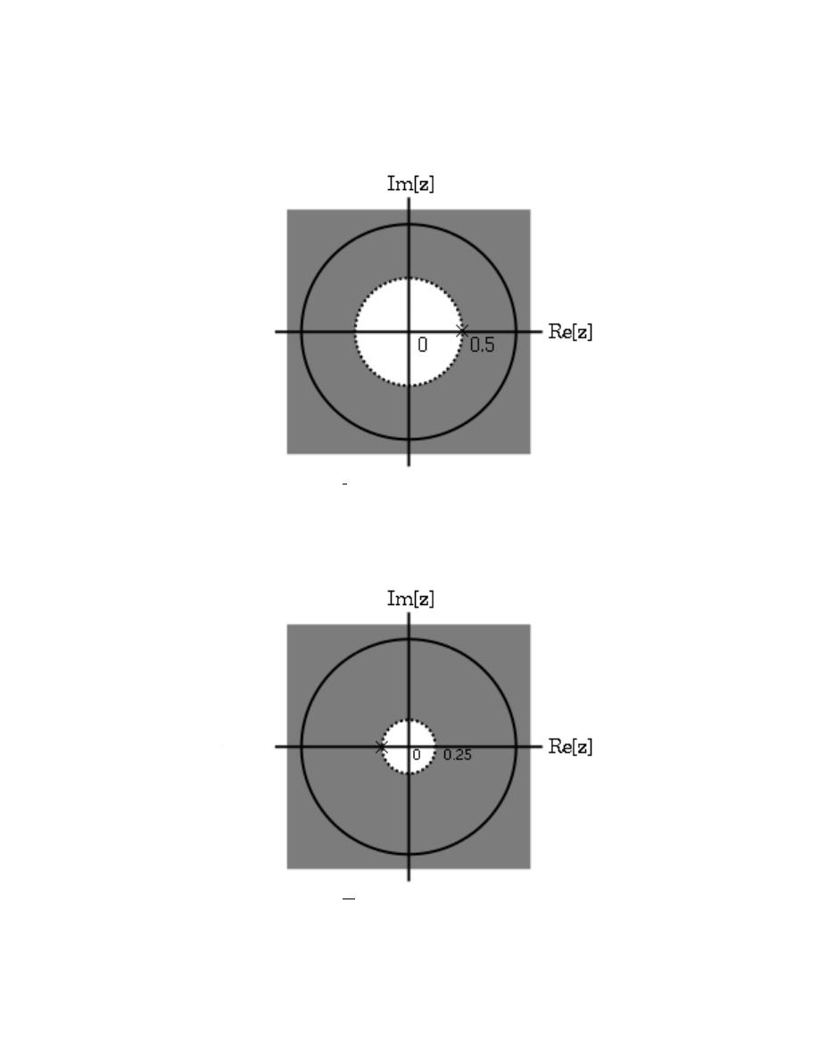
258
CHAPTER 12. Z-TRANSFORM AND DIGITAL FILTERING
Figure 12.13:
The ROC of
1
2
n
u [n]
Figure 12.14:
The ROC of
−1
4
n
u [n]
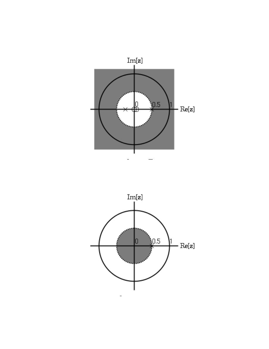
259
Figure 12.15:
The ROC of x
1
[n] =
1
2
n
u [n] +
−1
4
n
u [n]
Figure 12.16:
The ROC of −
1
2
n
u [−n − 1]
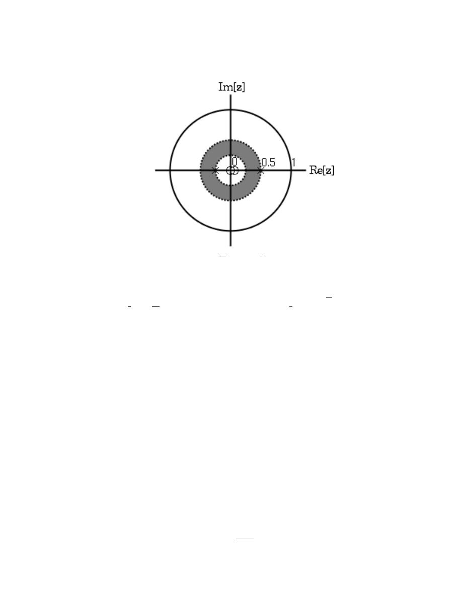
260
CHAPTER 12. Z-TRANSFORM AND DIGITAL FILTERING
Figure 12.17:
The ROC of x
2
[n] =
−1
4
n
u [n] −
1
2
n
u [−n − 1].
By observation it is again clear that there are two zeros, at 0 and
1
16
, and two
poles, at
1
2
, and
−1
4
. in ths case though, the ROC is |z| <
1
2
.
13.4 Inverse Z-Transrom
When using the z-transform
X (z) =
∞
X
n=−∞
x [n] z
−n
(12.30)
it is often useful to be able to find x [n] given X (z). There are at least 4 different methods
to do this:
1. - Inspection (Section 12.4.1)
2. - Partial-Fraction Expansion (Section 12.4.2)
3. - Power Series Expansion (Section 12.4.3)
4. - Contour Integration (Section 12.4.4)
12.4.1 Inspection Method
This ”method” is to basically become familiar with the z-transform pair tables and then
”reverse engineer”.
Example 12.5:
When given
X (z) =
z
z − α

261
with an ROC of
|z| > α
we could determine ”by inspection” that
x [n] = α
n
u [n]
12.4.2 Partial-Fraction Expansion Method
When dealing with linear time-invariant systems the z-transorm often in the form
X (z)
=
B(z)
A(z)
=
P
M
k=0
(
b
k
z
−k
)
P
N
k=0
(a
k
z
−k
)
(12.31)
This can also expressed as
X (z) =
a
0
b
0
Q
M
k=1
1 − c
k
z
−1
Q
N
k=1
(1 − d
k
z
−1
)
(12.32)
where c
k
reprisents the nonzero zeros of X (z) and d
k
reprisents the nonzero poles.
If M < N then X (z) can be reprisented as
X (z) =
N
X
k=1
A
k
1 − d
k
z
−1
(12.33)
This form allows for easy inversions of each term of the sum using the inspection method
(Section 12.4.1) and the transform table. Thus if the numerator is a polynomial then it is
necessary to use partial-fraction expansion to put X (z) in the above form. If M ≥ N then
X (z) can be expressed as
X (z) =
M −N
X
r=0
B
r
z
−r
+
P
N −1
k=0
b
’
k
z
−k
P
N
k=0
(a
k
z
−k
)
(12.34)
Example 12.6:
Find the inverse z-transform of
X (z) =
1 + 2z
−1
+ z
−2
1 + (−3z
−1
) + 2z
−2
where the ROC is |z| > 2. In this case M = N = 2, so we have to use long division
to get
X (z) =
1
2
+
1
2
+
7
2
z
−1
1 + (−3z
−1
) + 2z
−2
Next factor the denominator.
X (z) = 2 +
(−1) + 5z
−1
(1 − 2z
−1
) (1 − z
−1
)
Now do partial-fraction expansion.
X (z) =
1
2
+
A
1
1 − 2z
−1
+
A
2
1 − z
−1
=
1
2
+
9
2
1 − 2z
−1
+
−4
1 − z
−1
Now each term can be inverted using the inspection method and the z-transform
table. Thus, since the ROC is |z| > 2,
x [n] =
1
2
δ [n] +
9
2
2
n
u [n] + (−4u [n])

262
CHAPTER 12. Z-TRANSFORM AND DIGITAL FILTERING
12.4.3 Power Series Expansion Method
When the z-transform is defined as a power series in the form
X (z) =
∞
X
n=−∞
x [n] z
−n
(12.35)
then each term of the sequence x [n] can be determined by looking at the coefficients of the
respective power of z
−n
.
Example 12.7:
Now look at the z-transform of a finite-length sequence .
X (z)
=
z
2
1 + 2z
−1
1 −
1
2
z
−1
1 + z
−1
=
z
2
+
5
2
z +
1
2
+ − z
−1
(12.36)
In this case, since there were no poles, we multiplied the factors of X (z). Now, by
inspection, it is clear that
x [n] = δ [n + 2] +
5
2
δ [n + 1] +
1
2
δ [n] + (− (δ [n − 1]))
.
One of the advantages of the power series expansion method is that many functions
encountered in engineering problems have their power series’ tabulated. Thus functions
such as log, sin, exponent, sinh, etc, can be easily inverted.
Example 12.8:
Suppose
X (z) = log
n
1 + αz
−1
Noting that
log
n
(1 + x) =
∞
X
n=1
−1
n+1
x
n
n
Then
X (z) =
∞
X
n=1
−1
n+1
α
n
z
−n
n
Therefore
=
−1
n+1
α
n
n
if n ≥ 1
0 if n ≤ 0
12.4.4 Contour Integration Method
Without going in to much detail
x [n] =
1
2πj
I
r
X (z) z
n−1
dz
(12.37)
where r is a counter-clockwise countour in the ROC of X (z) encirciling the origin of the
z-plane. To further expand on this method of finding the inverse requires the knowledge of
complex variable theory and thus will not be addressed in this module.

263
13.5 Rational Functions
12.5.1 Introduction
When dealing with operations on polynomials, the term rational function is a simple way
to describe a particular relationship between two polynomials.
rational function :
For any two polynomails, A and B, their quotient is called
a rational function.
Example 98:
Below is a simple example of a basic rational function, f (x). Note that
the numerator and denomenator can be polynomials of any order, but the
rational function is undefined when the denomenator equals zero.
f (x) =
x
2
− 4
2x
2
+ x − 3
(12.38)
If you have begun to study the Z-transform, you should have noticed by now they are
all rational functions. Below we will look at some of the properties of rational functions and
how they can be used to reveal important characteristics about a z-transform, and thus a
signal or LTI system.
12.5.2 Properties of Rational Functions
In order to see what makes rational functions special, let us look at some of their basic
properties and characteristics. If you are familiar with rational functions and basic algebraic
properties, skip to the next section (Section 12.5.3) to see how rational functions are useful
when dealing with the z-transform.
12.5.2.1 Roots
To understand many of the following characteristics of a rational function, one must begin
by finding the roots of the rational function. In order to do this, let us factor both of the
polynomials so that the roots can be easily determined. Like all polynomials, the roots will
provide us with information on many key properties. The function below shows the results
of factoring the above rational function, Equation 12.38.
f (x) =
(x + 2) (x − 2)
(2x + 3) (x − 1)
(12.39)
Thus, the roots of the rational function are as follows:
Roots of the numerator are: {−2, 2}
Roots of the denomenator are: {−3, 1}
note:
In order to understand rational functions, it is essential to know and
understand the roots that make up the rational function.
12.5.2.2 Discontinuities
Because we are dealing with division of two polynomials, we must be aware of the values of
the variable that will cause the denominator of our fraction to be zero. When this happens,
the rational function becomes undefined, i.e. we have a discontinuity in the function. Be-
cause we have already solved for our roots, it is very easy to see when this occurs. When
the variable in the denomenator equals any of the roots of the denomenator, the function
becomes undefined.

264
CHAPTER 12. Z-TRANSFORM AND DIGITAL FILTERING
Example 12.9:
Continuing to look at our rational funtion above, Equation 12.38, we can see that
the function will have dicontinuites at the following points: x = {−3, 1}
In respect to the cartesian plane, we say that the discontinuities are the values along
the x-axis where the function in undefined. These discontinuities often appear as vertical
asymptotes on the graph to represent the values where the function is undefined.
12.5.2.3 Domain
Using the roots that we found above, the domain of the rational function can be easily
defined.
domain :
The group, or set, of values that are defined by a given function.
Example 100:
Using the rational function above, Equation 12.38, the domain can be
defined as any real number x where x does not equal 1 or negative 3.
Written out mathematical, we get the following:
{ x ∈ R |x 6= −3 x 6= 1}
(12.40)
12.5.2.4 Intercepts
The x-intercept is defined as the point(s) where f (x), i.e. the output of the rational
functions, equals zero. Because we have already found the roots of the equation this process
is very simple. From algebra, we know that the output will be zero whenever the numerator
of the rational function is equal to zero. Therefore, the function will have an x-intercept
wherever x equals one of the roots of the numerator.
The y-intercept occurs whenever x equals zero. This can be found by setting all the
values of x equal to zero and solving the rational function.
12.5.3 Rational Functions and the Z-Transform
As we have stated above, all z-transforms can be written as rational functions, which have
become the most common way of representing the z-transform. Because of this, we can use
the properties above, especially those of the roots, in order to reveal certain characteristics
about the signal or LTI system described by the z-transform.
Below is the general form of the z-transform written as a rational function:
X (z) =
b
0
+ b
1
z
−1
+ · · · + b
M
z
−M
a
0
+ a
1
z
−1
+ · · · + a
N
z
−N
(12.41)
If you have already looked at the module about Understanding Pole/Zero Plots and the
Z-transform, you should see how the roots of the rational function play an important role
in understanding the z-transform. The equation above, Equation 12.41, can be expressed in
factored form just as was done for the simple rational function above, see Equation 12.39.
Thus, we can easily find the roots of the numerator and denomenator of the z-transform.
The following two relationships become apparent:
Relationship of Roots to Poles and Zeros
• - The roots of the numerator in the rational function will be the zeros of the z-
transform
• - The roots of the denomenator in the rational function will be the poles of the
z-transform

265
12.5.4 Conclusion
Once we have used our knowledge of rational fuctions to find its roots, we can manipulate
a z-transform in a number of useful ways. We can apply this knowledge to representing an
LTI system graphically through a Pole/Zero Plot, or to analyze and design a digital filter
through Filter Design from the Z-Transform.
13.6 Difference Equation
12.6.1 Introduction
One of the most important concepts of DSP is to be able to properly represent the in-
put/ouput relationship to a given LTI system. A linear constant-coefficient difference
equation (LCCDE) serves as a way to express just this relationship in a discrete-time sys-
tem. Writing the sequence of inputs and outputs, which represent the charateristics of the
LTI system, as a difference equation help in understanding and manipulating a system.
difference equation :
An equation that shows the relationship between con-
secutive values of a sequence and the differences among them. They are often
rearranged as a recursive formula so that a systems output can be computed from
the input signal and past outputs.
Example 101:
y [n] + 7y [n − 1] + 2y [n − 2] = x [n] − 4x [n − 1]
(12.42)
12.6.2 General Formulas from the Difference Equation
As stated briefly in the definition above, a difference equation is a very useful tool in describ-
ing and calculating the output of the system described by the formula for a given sample n.
The key property of the difference equation is its ability to help easily find the transform,
H (z), of a system. In the following two subsections, we will look at the general form of the
difference equation and the general conversion to a z-transform directly from the difference
equation.
12.6.2.1 Difference Equation
The general form of a linear, constant-coefficient difference equation (LCCDE), is shown
below:
N
X
k=0
(a
k
y [n − k]) =
M
X
k=0
(b
k
x [n − k])
(12.43)
We can also write the general form to easily express a recursive output, which looks like
this:
y [n] = −
N
X
k=1
(a
k
y [n − k])
!
+
M
X
k=0
(b
k
x [n − k])
(12.44)
From this equation, note that y [n − k] represents the outputs and x [n − k] represents the
inputs. The value of N represents the order of the difference equation and corresponds to
the memory of the system being represented. Because this equation relies on past values of
the output, in order to compute a numerical solution, certain past outputs, referred to as
the initial conditions , must be known.

266
CHAPTER 12. Z-TRANSFORM AND DIGITAL FILTERING
12.6.2.2 Conversion to Z-Transform
Using the above formula, Equation 12.43, we can easily generalize the transfer function
, H (z), for any difference equation. Below are the steps taken to convert any difference
equation into its transfer function, i.e. z-transform. The first step involves taking the
Fourier Transform of all the terms in Equation 12.43. Then we use the linearity property to
pull the transform inside the summation and the time-shifting property of the z-transform to
change the time-shifting terms to exponentials. Once this is done, we arrive at the followin
equation: a
0
= 1.
Y (z) = −
N
X
k=1
a
k
Y (z) z
−k
!
+
M
X
k=0
b
k
X (z) z
−k
(12.45)
H (z)
=
Y (z)
X(z)
=
P
M
k=0
(
b
k
z
−k
)
1+
P
N
k=1
(a
k
z
−k
)
(12.46)
12.6.2.3 Conversion to Frequency Response
Once the z-transform has been calculated from the difference equation, we can go one step
further to define the frequency response of the system, or filter, that is being represented
by the difference equation.
note:
Remember that the reason we are dealing with these formulas is to be
able to aid us in filter design. A LCCDE is one of the easiest ways to represent
FIR filters. By being able to find the frequency response, we will be able to look
at the basic properties of any filter represented by a simple LCCDE.
Below is the general formula for the frequency response of a z-transform. The conversion is
simple a matter of taking the z-transform forumula, H (z), and replacing every instance of
z with e
jw
.
H (w)
=
H (z) |
z,z=e
jw
=
P
M
k=0
(
b
k
e
−(jwk)
)
P
N
k=0
(
a
k
e
−(jwk)
)
(12.47)
Once you understand the derivation of this formula, look at the module concerning Filter
Design from the Z-Transform for a look into how all of these ideas of the Z-transform,
Difference Equation, and Pole/Zero Plots play a role in filter design.
12.6.3 Example
Example 12.10:
Finding Difference Equation
Below is a basic example showing the opposite of the steps above: given a transfer
function one can easily calculate the systems difference equation.
H (z) =
(z + 1)
2
z −
1
2
z +
3
4
(12.48)
Given this transfer function of a time-domain filter, we want to find the difference
equation. To begin with, expand both polynomials and divide them by the highest
order z.
H (z)
=
(z+1)(z+1)
(
z−
1
2
)(
z+
3
4
)
=
z
2
+2z+1
z
2
+2z+1−
3
8
=
1+2z
−1
+z
−2
1+
1
4
z
−1
−
3
8
z
−2
(12.49)

267
From this transfer function, the coefficients of the two polynomials will be our a
k
and b
k
values found in the general difference equation formula, Equation 12.43.
Using these coefficients and the above form of the transfer function, we can easily
write the difference equation:
x [n] + 2x [n − 1] + x [n − 2] = y [n] +
1
4
y [n − 1] −
3
8
y [n − 2]
(12.50)
In our final step, we can rewrite the difference equation in its more common form
showing the recursive nature of the system.
y [n] = x [n] + 2x [n − 1] + x [n − 2] +
−1
4
y [n − 1] +
3
8
y [n − 2]
(12.51)
12.6.4 Solving a LCCDE
In order for a linear constant-coefficient difference equation to be useful in analyzing a LTI
system, we must be able to find the systems output based upon a known input, x (n), and
a set of initial conditions. Two common methods exist for solving a LCCDE: the direct
method and the indirect method , the later being based on the z-transform. Below we
will briefly discuss the formulas for solving a LCCDE using each of these methods.
12.6.4.1 Direct Method
The final solution to the output based on the direct method is the sum of two parts, expressed
in the following equation:
y (n) = y
h
(n) + y
p
(n)
(12.52)
The first part, y
h
(n), is referred to as the homogeneous solution and the second part,
y
h
(n), is referred to as particular solution . The following method is very similar to that
used to solve many differential equations, so if you have taken a differential calculus course
or used differential equations before then this should seem very familiar.
12.6.4.1.1 Homogeneous Solution
We begin by assuming that the input is zero, x (n) = 0. Now we simply need to solve the
homogeneous difference equation:
N
X
k=0
(a
k
y [n − k]) = 0
(12.53)
In order to solve this, we will make the assumption that the solution is in the form of an
exponential. We will use lambda, λ, to represent our exponential terms. We now have to
solve the following equation:
N
X
k=0
a
k
λ
n−k
= 0
(12.54)
We can expand this equation out and factor out all of the lambda terms. This will give us
a large polynomial in paranthesis, which is referred to as the characteristic polynomial .
The roots of this polynomial will be the key to solving the homogeneous equation. If there
are all distinct roots, then the general solution to the equation will be as follows:
y
h
(n) = C
1
(λ
1
)
n
+ C
2
(λ
2
)
n
+ · · · + C
N
(λ
N
)
n
(12.55)

268
CHAPTER 12. Z-TRANSFORM AND DIGITAL FILTERING
However, if the characteristic equation contains multiple roots then the above general solu-
tion will be slightly different. Below we have the modified version for an equation where λ
1
has K multiple roots:
y
h
(n) = C
1
(λ
1
)
n
+ C
1
n(λ
1
)
n
+ C
1
n
2
(λ
1
)
n
+ · · · + C
1
n
K−1
(λ
1
)
n
+ C
2
(λ
2
)
n
+ · · · + C
N
(λ
N
)
n
(12.56)
12.6.4.1.2 Particular Solution
The particular solution, y
p
(n), will be any solution that will solve the general difference
equation:
N
X
k=0
(a
k
y
p
(n − k)) =
M
X
k=0
(b
k
x (n − k))
(12.57)
In order to solve, our guess for the solution to y
p
(n) will take on the form of the input,
x (n). After guessing at a solution to the above equation involvling the particular solution,
one only needs to plug the solution into the difference equation and solve it out.
12.6.4.2 Indirect Method
The indirect method utilizes the relationship between the difference equation and z-transform,
discussed earlier (Section 12.6.2), to find a solution. The basic idea is to convert the differ-
ence equation into a z-transform, as described above (Section 12.6.2.2), to get the resulting
output, Y (z). Then by inverse tranforming this and using partial-fraction expansion, we
can arrive at the solution.
13.7 Understanding Pole/Zero Plots on the Z-Plane
12.7.1 Introduction to Poles and Zeros of the Z-Transform
Once the Z-transform of a system has been determined, one can use the information con-
tained in function’s polynomials to graphically represent the function and easily observe
many defining characteristics. The Z-transform will have the below structure, based on
Rational Functions:
X (z) =
P (z)
Q (z)
(12.58)
The two polynomials, P (z) and Q (z), allow us to find the poles and zeros of the Z-
Transform.
zeros :
1. The value(s) for z where P (z) = 0.
2. The complex frequencies that make the overall gain of the filter transfer function
zero.
poles :
1. The value(s) for z where Q (z) = 0.
2. The complex frequencies that make the overall gain of the filter transfer function
infinite.
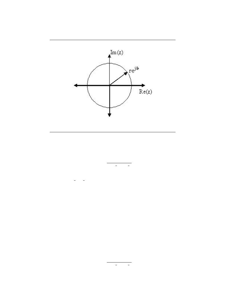
269
Z-Plane
Figure 12.18
Example 12.11:
Below is a simple transfer function with the poles and zeros shown below it.
H (z) =
z + 1
z −
1
2
z +
3
4
The zeros are: {−1}
The poles are:
1
2
, −
3
4
12.7.2 The Z-Plane
Once the poles and zeros have been found for a given Z-Transform, they can be plotted onto
the Z-Plane. The Z-plane is a complex plane with an imaginary and real axis referring to
the complex-valued variable z. The position on the complex plane is given by re
jθ
and the
angle from the positive, real axis around the plane is denoted by θ. When mapping poles
and zeros onto the plane, poles are denoted by an ”x” and zeros by an ”o”. The below figure
shows the Z-Plane, and examples of plotting zeros and poles onto the plane can be found in
the following section.
12.7.3 Examples of Pole/Zero Plots
This section lists several examples of finding the poles and zeros of a transfer function and
then plotting them onto the Z-Plane.
Example 12.12:
Simple Pole/Zero Plot
H (z) =
z
z −
1
2
z +
3
4
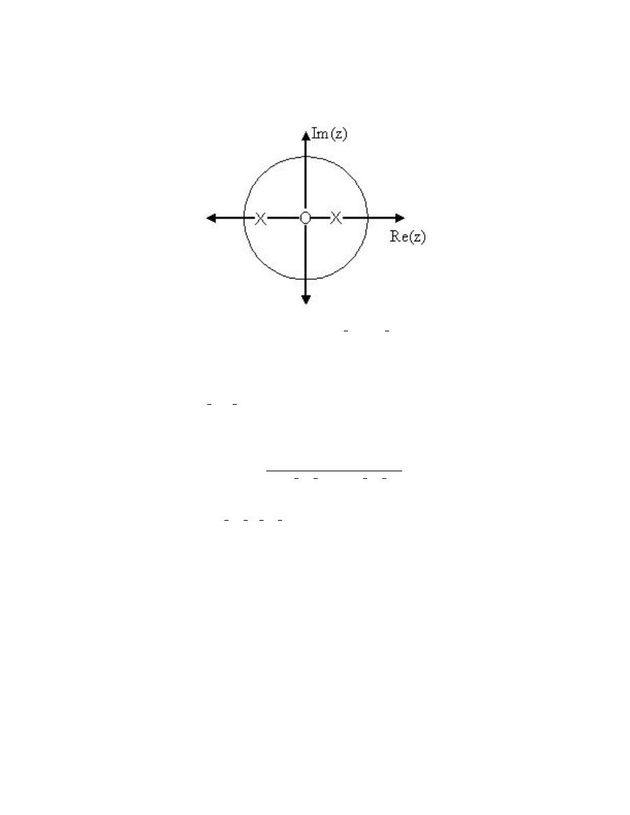
270
CHAPTER 12. Z-TRANSFORM AND DIGITAL FILTERING
Pole/Zero Plot
Figure 12.19:
Using the zeros and poles found from the transfer function, the one zero
is mapped to zero and the two poles are placed at
1
2
and −
3
4
The zeros are: {0}
The poles are:
1
2
, −
3
4
Example 12.13:
Complex Pole/Zero Plot
H (z) =
(z − j) (z + j)
z −
1
2
−
1
2
j
z −
1
2
+
1
2
j
The zeros are: {j, −j}
The poles are:
−1,
1
2
+
1
2
j,
1
2
−
1
2
j
MATLAB - If access to MATLAB is readily available, then you can use its functions to
easily create pole/zero plots. Below is a short program that plots the poles and zeros from
the above example onto the Z-Plane.
% Set up vector for zeros
z = [j ; -j];
% Set up vector for poles
p = [-1 ; .5+.5j ; .5-.5j];
figure(1);
zplane(z,p);
title(’Pole/Zero Plot for Complex Pole/Zero Plot Example’);
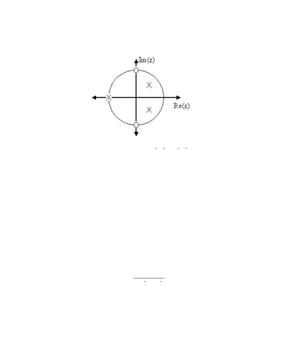
271
Pole/Zero Plot
Figure 12.20:
Using the zeros and poles found from the transfer function, the zeros
are mapped to ±j, and the poles are placed at −1,
1
2
+
1
2
j and
1
2
−
1
2
j
12.7.4 Pole/Zero Plot and Region of Convergance
The region of convergence (ROC) for X (z) in the complex Z-plane can be determined from
the pole/zero plot. Although several regions of convergence may be possible, where each one
corresponds to a different impulse response, there are some choices that are more practical.
A ROC can be chosen to make the transfer function causal and/or stable depending on the
pole/zero plot.
Filter Properties from ROC
• - If the ROC extends outward from the outermost pole, then the system is causal .
• - If the ROC includes the unit circle, then the system is stable .
Below is a pole/zero plot with a possible ROC of the Z-transform in the Simple Pole/Zero
Plot (Example 12.12) discussed earlier. The shaded region indicates the ROC chosen for
the filter. From this figure, we can see that the filter will be both causal and stable since
the above listed conditions are both met.
Example 12.14:
H (z) =
z
z −
1
2
z +
3
4
12.7.5 Frequency Response and the Z-Plane
The reason it is helpful to understand and create these pole/zero plots is due to their ability
to help us easily design a filter. Based on the location of the poles and zeros, the magnitude
response of the filter can be quickly understood.
Also, by starting with the pole/zero
plot, one can design a filter and obtain its transfer function very easily. Refer to this for
information on the relationship between the pole/zero plot and the frequency response.
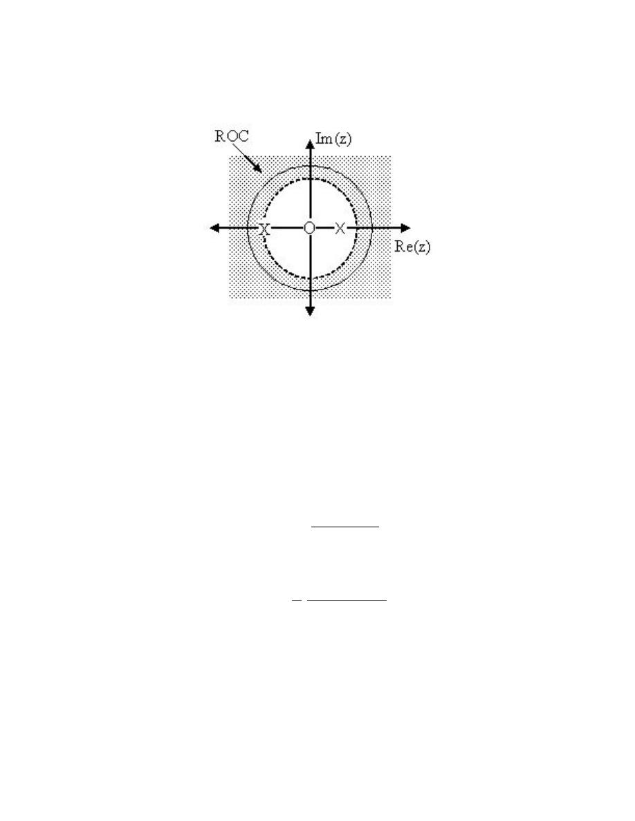
272
CHAPTER 12. Z-TRANSFORM AND DIGITAL FILTERING
Region of Convergence for the Pole/Zero Plot
Figure 12.21:
The shaded area represents the chosen ROC for the transfer function.
13.8 Filter Design using the Pole/Zero Plot of a Z-Transform
12.8.1 Estimating Frequency Response from Z-Plane
One of the motivating factors for analyzing the pole/zero plots is due to their relationship
to the frequency response of the system. Based on the position of the poles and zeros,
one can quickly determine the frequency response. This is a result of the correspondance
between the frequency response and the transfer function evaluated on the unit circle in the
pole/zero plots. The frequency response, or DTFT, of the system is defined as:
H (w)
=
H (z) |
z,z=e
jw
=
P
M
k=0
(
b
k
e
−(jwk)
)
P
N
k=0
(
a
k
e
−(jwk)
)
(12.59)
Next, by factoring the transfer function into poles and zeros and multiplying the numerator
and denominator by e
jw
we arrive at the following equations:
H (w) = |
b
0
a
0
|
Q
M
k=1
|e
jw
− c
k
|
Q
N
k=1
(|e
jw
− d
k
|)
(12.60)
From Equation 12.60 we have the frequency response in a form that can be used to interpret
physical characteristics about the filter’s frequency response. The numerator and denomi-
nator contain a product of terms of the form |e
jw
− h|, where h is either a zero, denoted
by c
k
or a pole, denoted by d
k
. Vectors are commonly used to represent the term and its
parts on the complex plane. The pole or zero, h, is a vector from the origin to its location
anywhere on the complex plane and e
jw
is a vector from the origin to its location on the
unit circle. The vector connecting these two points, |e
jw
− h|, connects the pole or zero
location to a place on the unit circle dependent on the value of w. From this, we can begin
to understand how the magnitude of the frequency response is a ratio of the distances to
the poles and zero present in the z-plane as w goes from zero to pi. These characteristics

273
allow us to interpret |H (w) | as follows:
|H (w) | = |
b
0
a
0
|
Q ”distancesfromzeros”
Q ”distancesfrompoles”
(12.61)
In conclusion, using the distances from the unit circle to the poles and zeros, we can plot
the frequency response of the system. As w goes from 0 to 2π, the following two properties,
taken from the above equations, specify how one should draw |H (w) |.
While moving around the unit circle...
1. - if close to a zero, then the magnitude is small. If a zero is on the unit circle, then
the frequency response is zero at that point.
2. - if close to a pole, then the magnitude is large. If a pole is on the unit circle, then
the frequency response goes to infinity at that point.
12.8.2 Drawing Frequency Response from Pole/Zero Plot
Let us now look at several examples of determing the magnitude of the frequency response
from the pole/zero plot of a z-transform. If you have forgotten or are unfamiliar with
pole/zero plots, please refer back to the Pole/Zero Plots module.
Example 12.15:
In this first example we will take a look at the very simple z-transform shown
below:
H (z) = z + 1 = 1 + z
−1
H (w) = 1 + e
−(jw)
For this example, some of the vectors represented by |e
jw
−h|, for random values of
w, are explicitly drawn onto the complex plane shown in the figure (pg ??) below.
These vectors show how the amplitude of the frequency response changes as w goes
from 0 to 2π, and also show the physical meaning of the terms in Equation 12.60
above. One can see that when w = 0, the vector is the longest and thus the
frequency respone will have its largest amplitude here. As w approaches π, the
length of the vectors decrease as does the amplitude of |H (w) |. Since there are
no poles in the transform, there is only this one vector term rather than a ratio as
seen in Equation 12.60.
Example 12.16:
For this example, a more complex transfer function is analyzed in order to represent
the system’s frequency response.
H (z) =
z
z −
1
2
=
1
1 −
1
2
z
−1
H (w) =
1
1 −
1
2
e
−(jw)
Below we can see the two figures described by the above equations. The figure on
the left represents the basic pole/zero plot of the z-transform, H (w). The second
figure shows the magnitude of the frequency response. From the formulas and
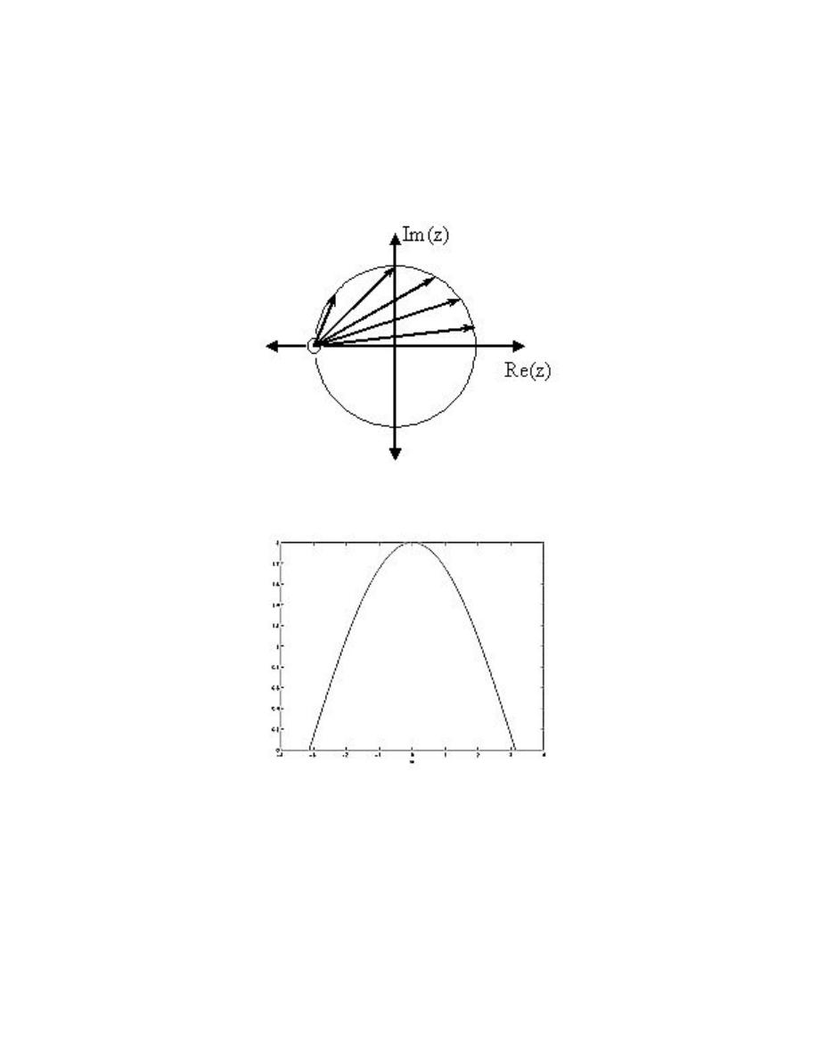
274
CHAPTER 12. Z-TRANSFORM AND DIGITAL FILTERING
(a) Pole/Zero Plot
(b) Frequency Respone: —H(w)—
Figure 12.22:
The first figure represents the pole/zero plot with a few representative
vectors graphed while the second shows the frequency response with a peak at +2 and
graphed between plus and minus pi.

275
statements in the previous section, we can see that when w = 0 the frequency will
peak since it is at this value of w that the pole is closest to the unit circle. The
ratio from Equation 12.60 helps us see the mathematics behind this conclusion and
the relationship between the distances from the unit circle and the poles and zeros.
As w moves from 0 to π, we see how the zero begins to mask the effects of the pole
and thus force the frequency response closer to 0.
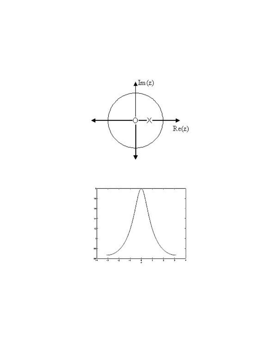
276
CHAPTER 12. Z-TRANSFORM AND DIGITAL FILTERING
(a) Pole/Zero Plot
(b) Frequency Respone: —H(w)—
Figure 12.23:
The first figure represents the pole/zero plot while the second shows the
frequency response with a peak at +2 and graphed between plus and minus pi.

Chapter 13
Homework Sets
14.1 Homework #1
due date:
Noon, Thursday, September 5, 2002
13.1.1 Assignment 1
Homework, tests, and solutions from previous offerings of this course are off limits, under
the honor code.
13.1.1.1 Problem 1
Form a study group of 3-4 members. With your group, discuss and synthesize the major
themes of this week of lectures. Turn in a one page summary of your discussion. You need
turn in only one summary per group, but include the names of all group members. Please
do not write up just a ”table of contents.”
13.1.1.2 Problem 2
Construct a WWW page (with your picture) and email Mike Wakin (wakin@rice.edu) your
name (as you want it to appear on the class web page) and the URL. If you need assistance
setting up your page or taking/scanning a picture (both are easy!), ask your classmates.
13.1.1.3 Problem 3: Learning Styles
Follow this learning styles link
1
(also found on the Elec 301 web page
2
) and learn about the
basics of learning styles. Write a short summary of what you learned. Also, complete the
“Index of learning styles” self-scoring test on the web and bring your results to class.
13.1.1.4 Problem 4
Make sure you know the material in Lathi, Chapter B, Sections 1-4, 6.1, 6.2, 7. Specifically,
be sure to review topics such as:
• - complex arithmetic (adding, multiplying, powers)
• - finding (complex) roots of polynomials
1
http://www2.ncsu.edu/unity/lockers/users/f/felder/public/Learning Styles.html
2
http://www-dsp.rice.edu/courses/elec301/
277

278
CHAPTER 13. HOMEWORK SETS
• - complex plane and plotting roots
• - vectors (adding, inner products)
13.1.1.5 Problem 5: Complex Number Applet
Reacquaint yourself with complex numbers by going to the course applets web page
3
and
clicking on the Complex Numbers applet (may take a few seconds to load).
(a) Change the default add function to exponential (exp). Click on the complex plane
to get a blue arrow, which is your complex number z. Click again anywhere on the complex
plane to get a yellow arrow, which is equal to e
z
. Now drag the tip of the blue arrow along
the unit circle on with |z| = 1 (smaller circle). For which values of z on the unit circle does
e
z
also lie on the unit circle? Why?
(b) Experiment with the functions absolute (abs), real part (re), and imaginary part
(im) and report your findings.
13.1.1.6 Problem 6: Complex Arithmetic
Reduce the following to the cartesian form, a + jb. Do not use your calculator!
(a)
−1−j
√
2
20
(b)
1+2j
3+4j
(c)
1+
√
3j
√
3−j
(d)
√
j
(e) j
j
13.1.1.7 Problem 7: Roots of Polynomials
Find the roots of each of the following polynomials (show your work). Use MATLAB to
check your answer with the roots command and to plot the roots in the complex plane.
Mark the root locations with an ’o’. Put all of the roots on the same plot and identify the
corresponding polynomial (a, b, etc...).
(a) z
2
− 4z
(b) z
2
− 4z + 4
(c) z
2
− 4z + 8
(d) z
2
+ 8
(e) z
2
+ 4z + 8
(f) 2z
2
+ 4z + 8
13.1.1.8 Problem 8: Nth Roots of Unity
e
j2π
N
is called an Nth Root of Unity .
(a) Why?
(b) Let z = e
j2π
7
. Draw
z, z
2
, . . . , z
7
in the complex plane.
(c) Let z = e
j4π
7
. Draw
z, z
2
, . . . , z
7
in the complex plane.
3
http://www.dsp.rice.edu/courses/elec301/applets.shtml

279
13.1.1.9 Problem 9: Writing Vectors in Terms of Other Vectors
A pair of vectors u ∈ C
2
and v ∈ C
2
are called linearly independent if
αu + βv = 0 if and only if α = β = 0
It is a fact that we can write any vector in C
2
as a weighted sum (or linear combination
) of any two linearly independent vectors, where the weights α and β are complex-valued.
(a) Write
3 + 4j
6 + 2j
as a linear combination of
1
2
and
−5
3
. That is, find α
and β such that
3 + 4j
6 + 2j
= α
1
2
+ β
−5
3
(b) More generally, write x =
x
1
x
2
as a linear combination of
1
2
and
−5
3
.
We will denote the answer for a given x as α (x) and β (x).
(c) Write the answer to (a) in matrix form, i.e. find a 2×2 matrix A such that
A
x
1
x
2
=
α (x)
β (x)
(d) Repeat (b) and (c) for a general set of linearly independent vectors u and v.
13.1.1.10 Problem 10: Fun with Fractals
A Julia set J is obtained by characterizing points in the complex plane. Specifically, let
f (x) = x
2
+ µ with µ complex, and define
g
0
(x) = x
g
1
(x) = f (g
0
(x)) = f (x)
g
2
(x) = f (g
1
(x)) = f (f (x))
..
.
g
n
(x) = f (g
n−1
(x))
Then for each x in the complex plane, we say x ∈ J if the sequence
{|g
0
(x) |, |g
1
(x) |, |g
2
(x) |, . . . }
does not tend to infinity. Notice that if x ∈ J , then each element of the sequence {g
0
(x) , g
1
(x) , g
2
(x) , . . . }
also belongs to J .
For most values of µ, the boundary of a Julia set is a fractal curve - it contains ”jagged”
detail no matter how far you zoom in on it. The well-known Mandelbrot set contains all
values of µ for which the corresponding Julia set is connected.
(a) Let µ = −1. Is x = 1 in J ?
(b) Let µ = 0. What conditions on x ensure that x belongs to J ?
(c) Create an approximate picture of a Julia set in MATLAB. The easiest way is to
create a matrix of complex numbers, decide for each number whether it belongs to J , and
plot the results using the imagesc command. To determine whether a number belongs to
J , it is helpful to define a limit N on the number of iterations of g. For a given x, if the
magnitude |g
n
(x) | remains below some threshold M for all 0 ≤ n ≤ N , we say that x
belongs to J . The code below will help you get started:

280
CHAPTER 13. HOMEWORK SETS
N = 100;
% Max # of iterations
M = 2;
% Magnitude threshold
mu = -0.75;
% Julia parameter
realVals = [-1.6:0.01:1.6];
imagVals = [-1.2:0.01:1.2];
xVals = ones(length(imagVals),1) * realVals + ...
j*imagVals’*ones(1,length(realVals));
Jmap = ones(size(xVals));
g = xVals;
% Start with g0
% Insert code here to fill in elements of Jmap.
Leave a ’1’
% in locations where x belongs to J, insert ’0’ in the
% locations otherwise.
It is not necessary to store all 100
% iterations of g!
imagesc(realVals, imagVals, Jmap);
colormap gray;
xlabel(’Re(x)’);
ylabel(’Imag(x)’);
This creates the following picture for µ = −0.75, N = 100, and M = 2.
Using the same values for N, M, and x, create a picture of the Julia set for µ = −0.391 −
0.587j. Print out this picture and hand it in with your MATLAB code.
Just for Fun:
Try assigning differet color values to Jmap.
For example,
let Jmap indicate the first iteration when the magnitude exceeds M. Tip: try
imagesc(log(Jmap)) and colormap jet for a neat picture.
14.2 Homework #1 Solutions
13.2.1 Problem #1
No solutions provided.
13.2.2 Problem #2
No solutions provided.
13.2.3 Problem #3
No solutions provided.
13.2.4 Problem #4
No solutions provided.
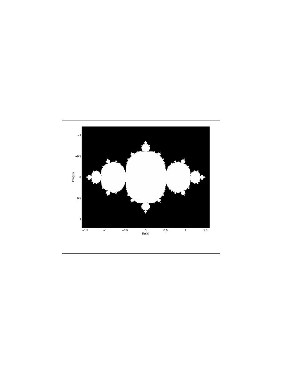
281
Figure 13.1:
Example image where the x-axis is Re(x) and the y-axis is Imag(x).

282
CHAPTER 13. HOMEWORK SETS
13.2.5 Problem #5
13.2.5.1 Part (a)
e
z
lies on the unit circle for z = ±j. When z = ±j,
e
z
= e
±j
= cos (±1) + jsin (±1)
e
±j
=
cos
2
(±1) + sin
2
(±1)
1
2
=
1
(13.1)
which gives us the unit circle!
Think of it this way: for z = σ + jθ, you want a σ = 0 so that e
σ+jθ
reduces as
e
σ+jθ
= e
σ
e
jθ
= e
0
e
jθ
= e
jθ
We know by Euler’s formula (Section 2.6.2) that
e
jθ
= cos (θ) + jsin (θ)
The magnitude of this is given by sin
2
(θ) + cos
2
(θ), which is 1 (which implies that e
jθ
is
on the unit circle).
So, we know we want to pick a z = Ajθ that is on the unit circle (from the problem
statement), so we have to choose A = ±1 to get unit magnitude.
13.2.5.2 Part (b)
• - abs gives magnitude of complex number
• - re gives real part of complex number
• - im gives imaginary part of complex number
13.2.6 Problem #6
13.2.6.1 Part (a)
−1 − j
√
2
20
=
√
2e
5π
4
√
2
!
20
=
e
5π
4
20
= e
j25π
= e
jπ
= −1
13.2.6.2 Part (b)
1 + 2j
3 + 4j
=
1 + 2j
3 + 4j
3 − 4j
3 − 4j
=
3 + 6j − (4j + 8)
9 + 16
=
11 + 2j
25
=
11
25
+
2
25
j
13.2.6.3 Part (c)
1 +
√
3j
√
3 − j
=
2e
j
π
3
2e
j
−π
6
= e
j
π
2
= j
13.2.6.4 Part (d)
p
j = e
j
π
2
1
2
= e
j
π
4
= cos
π
4
+ jsin
π
4
=
√
2
2
+
√
2
2
j

283
13.2.6.5 Part (e)
j
j
= e
j
π
2
j
= e
j
2 π
2
= e
−π
2
13.2.7 Problem #7
13.2.7.1 Part (a)
z
2
− 4z = z (z − 4)
Roots of z = {0, 4}
13.2.7.2 Part (b)
z
2
− 4z + 4 = (z − 2)
2
Roots of z = {2, 2}
13.2.7.3 Part (c)
z
2
− 4z + 8
Roots of z =
4 ±
√
16 − 32
2
= 2 ± 2j
13.2.7.4 Part (d)
z
2
+ 8
Roots of z =
±
√
−32
2
= ±2
√
2j
13.2.7.5 Part (e)
z
2
+ 4z + 8
Roots of z =
−4 ±
√
16 − 32
2
= −2 ± 2j
13.2.7.6 Part (f )
2z
2
+ 4z + 8
Roots of z =
−4 ±
√
16 − 64
4
= −1 ±
√
3j
13.2.7.7 Matlab Code and Plot
%%%%%%%%%%%%%%%
%%%%% PROBLEM 7
%%%%%%%%%%%%%%%
rootsA = roots([1 -4 0])
rootsB = roots([1 -4 4])
rootsC = roots([1 -4 8])
rootsD = roots([1 0 8])
rootsE = roots([1 4 8])
rootsF = roots([2 4 8])
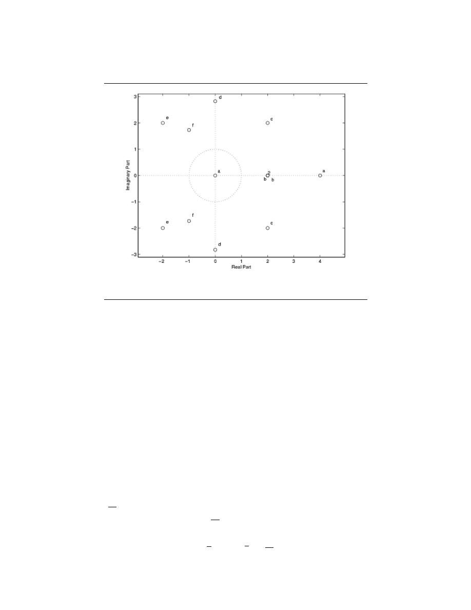
284
CHAPTER 13. HOMEWORK SETS
Figure 13.2:
Plot of all the roots.
zplane([rootsA; rootsB; rootsC; rootsD; rootsE; rootsF]);
gtext(’a’)
gtext(’a’)
gtext(’b’)
gtext(’b’)
gtext(’c’)
gtext(’c’)
gtext(’d’)
gtext(’d’)
gtext(’e’)
gtext(’e’)
gtext(’f’)
gtext(’f’)
13.2.8 Problem #8
13.2.8.1 Part (a)
Raise e
j2π
N
to the Nth power.
e
j2π
N
N
= e
j2π
= 1
note:
Similarly,
(1)
1
N
= e
j2π
1
N
= e
j2π
N

285
13.2.8.2 Part (b)
For z = e
j2π
7
,
z
k
=
e
j2π
7
k
= e
j2π
k
7
We will have points on the unit circle with angle of
2π
7
,
2π2
7
, . . . ,
2π7
7
. The code used to
plot these in MATLAB can be found below, followed by the plot.
%%%%%%%%%%%%%%%
%%%%% PROBLEM 8
%%%%%%%%%%%%%%%
%%% Part (b)
figure(1);
clf;
hold on;
th = [0:0.01:2*pi];
unitCirc = exp(j*th);
plot(unitCirc,’--’);
for k = 1:7
z = exp(j*2*pi*k/7);
plot(z,’o’);
text(1.2*real(z),1.2*imag(z),strcat(’z^’,num2str(k)));
end
xlabel(’real part’);
ylabel(’imag part’);
title(’Powers of exp(j2\pi/7) on the unit circle’);
axis([-1.5 1.5 -1.5 1.5]);
axis square;
13.2.8.3 Part (c)
For z = e
j4π
7
,
z
k
=
e
j4π
7
k
= e
j2π
2k
7
Where we have
z, z
2
, . . . , z
7
=
n
e
j2π
2
7
, e
j2π
4
7
, e
j2π
6
7
, e
j2π
1
7
, e
j2π
3
7
, e
j2π
5
7
, 1
o
The code used to plot these in MATLAB can be found below, followed by the plot.
%%% Part (c)
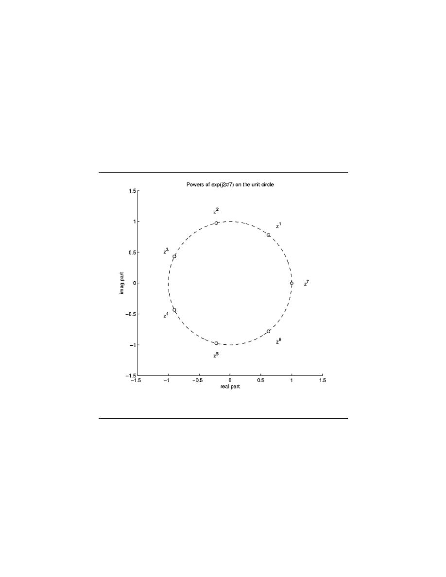
286
CHAPTER 13. HOMEWORK SETS
Figure 13.3:
MATLAB plot of part (b).

287
figure(1);
clf;
hold on;
th = [0:0.01:2*pi];
unitCirc = exp(j*th);
plot(unitCirc,’--’);
for k = 1:7
z = exp(j*4*pi*k/7);
plot(z,’o’);
text(1.2*real(z),1.2*imag(z),strcat(’z^’,num2str(k)));
end
xlabel(’real part’);
ylabel(’imag part’);
title(’Powers of exp(j4\pi/7) on the unit circle’);
axis([-1.5 1.5 -1.5 1.5]);
axis square;
13.2.9 Problem #9
13.2.9.1 Part (a)
3 + 4j
6 + 2j
= α
1
2
+ β
−5
3
To solve for β we must solve the following system of equations:
α − 5β = 3 + 4j
2α + 3β = 6 + 2j
If we multiply the top equation by −2 we will get the following, which allows us to cancel
out the alpha terms:
−2α + 10β = −6 − 8j
2α + 3β = 6 + 2j
And now we have,
13β = −6j
β =
−6
13
j
And to solve for α we have the following equation:
α
=
3 + 4j + 5β
=
3 + 4j + 5
−6
13
j
=
3 +
22
13
j
(13.2)

288
CHAPTER 13. HOMEWORK SETS
Figure 13.4:
MATLAB plot of part (c).

289
13.2.9.2 Part (b)
x
1
x
2
= α
1
2
+ β
−5
3
x
1
= α − 5β
x
2
= 2α + 3β
Solving for α and β we get:
α (x) =
3x
1
+ 5x
2
13
β (x) =
−2x
1
+ x
2
13
13.2.9.3 Part (c)
α (x)
β (x)
=
3
13
5
13
−2
13
1
13
x
1
x
2
13.2.9.4 Part (d)
Write u =
u
1
u
2
and v =
v
1
v
2
. Then solve
x
1
x
2
= α
u
1
u
2
+ β
v
1
v
2
which corresponds to the system of equations
x
1
= αu
1
+ βv
1
x
2
= αu
2
+ βv
2
Solving for α and β we get
α (x) =
v
2
x
1
− v
1
x
2
u
1
v
2
− u
2
v
1
β (x) =
u
2
x
1
− u
1
x
2
v
1
u
2
− u
1
v
2
For the matrix A we get
A =
1
u
1
v
2
− u
2
v
1
v
2
−v
1
−u
2
u
1
13.2.10 Problem #10
13.2.10.1 Part (a)
If u = −1, then f (x) = x
2
− 1. Examine the sequence {g
0
(x) , g
1
(x) , . . . }:
g
0
(x) = 1
g
1
(x) = 1
2
− 1 = 0
g
2
(x) = 0
2
− 1 = −1
g
3
(x) = (−1)
2
− 1 = 0
g
4
(x) = 0
2
− 1 = −1
..
.
The magnitude sequence remains bounded so x = 1 belongs to J .

290
CHAPTER 13. HOMEWORK SETS
13.2.10.2 Part (b)
If u = 0, then f (x) = x
2
. So we have
g
0
(x) = x
g
1
(x) = x
2
g
2
(x) = x
2
2
= x
4
..
.
g
n
(x) = x
2
n
= x
2n
Writing x = re
jθ
, we have g
n
(x) = x
2n
= r
2n
e
jθ2n
, and so we have
|g
n
(x) | = r
2n
The magnitude sequence blows up if and only if r > 1. Thus x belongs to J if and only if
|x| ≤ 1. So, J corresponds to the unit disk.
13.2.10.3 Part (c)
%%%%%%%%%%%%%%%%
%%%%% PROBLEM 10
%%%%%%%%%%%%%%%%
%%% Part (c) - solution code
N = 100;
% Max # of iterations
M = 2;
% Magnitude threshold
mu = -0.391 - 0.587*j;
% Julia parameter
realVals = [-1.6:0.01:1.6];
imagVals = [-1.2:0.01:1.2];
xVals = ones(length(imagVals),1)*realVals + ...
j*imagVals’*ones(1,length(realVals));
Jmap = ones(size(xVals));
g = xVals; % Start with g0
for n = 1:N
g = g.^2 + mu;
big = (abs(g) >
M);
Jmap = Jmap.*(1-big);
end
imagesc(realVals,imagVals,Jmap); colormap gray;
xlabel(’Re(x)’); ylabel(’Imag(x)’);
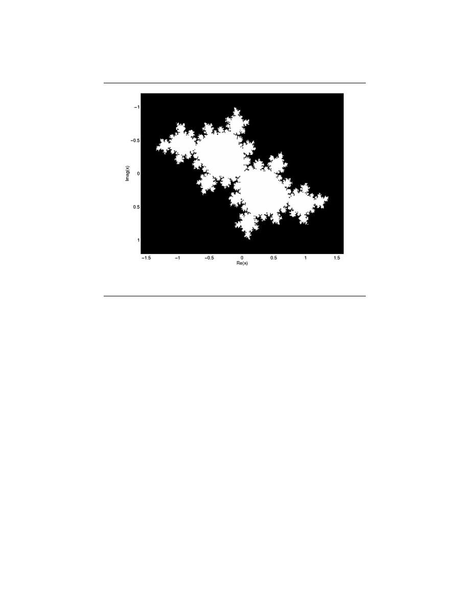
291
Figure 13.5:
MATLAB plot of part (c).
13.2.10.4 Just for Fun Solution
%%% Just for fun code
N = 100;
% Max # of iterations
M = 2;
% Magnitude threshold
mu = -0.391 - 0.587*j;
% Julia parameter
realVals = [-1.6:0.005:1.6];
imagVals = [-1.2:0.005:1.2];
xVals = ones(length(imagVals),1)*realVals + ...
j*imagVals’*ones(1,length(realVals));
Jmap = zeros(size(xVals));
% Now, we put zeros in the ’middle’, for a
% cool effect.
g = xVals; % Start with g0
for n = 1:N
g = g.^2 + mu;
big = (abs(g) >
M);
notAlreadyBig = (Jmap == 0);
Jmap = Jmap + n*(big.*notAlreadyBig);
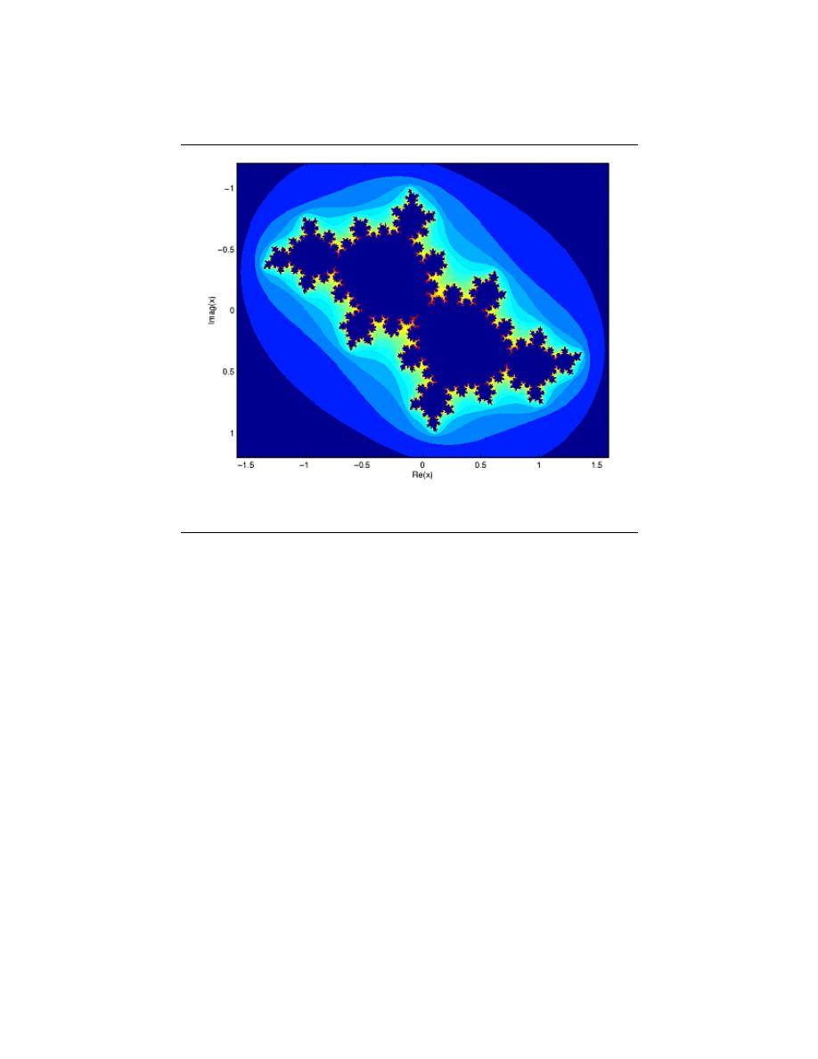
292
CHAPTER 13. HOMEWORK SETS
Figure 13.6:
MATLAB plot.
end
imagesc(realVals,imagVals,log(Jmap));colormap jet;
xlabel(’Re(x)’); ylabel(’Imag(x)’);

293
Index of Keywords and
Terms
Keywords are listed by the section
with that keyword (page numbers are
in parentheses). Keywords do not nec-
essarily appear in the text of the page.
They are merely associated with that
section. Ex.
apples, § 1.1 (1) Terms
are referenced by the page they appear
on. Ex.
apples, 1
”
”standard basis”, 69
A
alias, § 11.5(223), § 11.6(227)
aliasing, § 8.2(154), § 11.5(223), 224,
§ 11.6(227)
almost everywhere, § 6.11(108)
alphabet, § 3.4(23), 26
analog, § 3.3(14), 17, 23, § 10.6(200),
§ 10.7(202)
analog signal, § 2.1(3)
analysis, 88
anitcausal, 17
Anti-Aliasing, § 11.6(227)
anticausal, § 3.3(14)
aperiodic, § 3.3(14)
approximation, § 7.13(151)
B
bandlimited, 213, § 11.2(215)
baraniuk, § 1(1), § 14.2(280)
bases, § 7.7(131)
basis, § 3.6(30), § 5.1(65), 68, 68, 69,
§ 5.4(76), § 7.7(131), § 7.8(135), 135,
§ 7.9(139), § 7.10(140), § 7.11(143),
§ 8.2(154), 160, § 8.3(163), 219
basis matrix, § 7.8(135), 136
best approximates, 151
BIBO, § 3.1(7), § 3.9(40)
bilateral Laplace transform pair, 235
bilateral z-transform, 247
bounded input bounded output,
§ 3.9(40)
bounded input-bounded output
(BIBO), 9
boxcar filter, 37
butterfly, § 8.9(185), 186
C
cartesian, 278
cascade, § 3.2(9)
cauch-schwarz, § 7.5(120)
cauchy, § 7.5(120)
cauchy-schwarz inequality, § 7.5(120),
121
causal, § 3.1(7), 9, § 3.2(9), § 3.3(14),
17, 271
characteristic polynomial, 267
circular, § 6.7(100), § 8.6(178)
circular convolution, § 6.5(93),
§ 6.7(100), § 8.6(178), 178
circular shift, § 8.5(168)
circular shifting, § 8.5(168), 168
Circular Shifts, 168
cirular convolution, § 8.5(168)
classification, § 3.1(7)
classification of systems, § 3.1(7)
coefficient, § 6.2(83)
coefficient vector, § 7.8(135), 137
coefficients, § 13.6(265)
commutative, 46, 54, 58
complex, § 3.4(23), § 3.6(30)
complex amplitude, 31
complex continuous-time exponential
signal, 30
complex exponential, 26, § 3.6(30), 30,
§ 6.2(83)
complex exponential sequence, 25
complex plane, § 3.6(30)
complex sinusoid, § 3.6(30), § 8.2(154)
complex vector space, § 7.1(113), 113
complex-valued, § 3.4(23)
complex-valued function, 236, 236
complexity, § 8.7(183), 183, § 8.9(185)
composite, 186
computational advantage, 185
computational complexity, § 8.7(183)
conjugates, 160
continous time, 211
continuos time, § 11.1(211)
continuous, § 3.1(7), 17, 106
continuous frequency, § 10.4(199),
§ 10.8(204)
continuous system, 7
continuous time, § 3.3(14), § 3.5(26),
§ 3.9(40), § 4.2(46), § 6.11(108),
§ 8.1(153), § 10.3(199), § 10.8(204),
§ 10.9(207), § 11.7(228), § 12.1(235),
§ 12.2(239), § 12.3(239), § 12.4(240),
§ 12.6(243)
continuous time signal, § 11.7(228)
continuous-time, § 10.8(204),
§ 10.9(207)

294
CHAPTER 13. HOMEWORK SETS
Continuous-Time Fourier Transform,
205
control theory, 246
converge, § 6.9(104), § 9.3(194)
convergence, § 6.9(104), 106,
§ 9.1(189), § 9.2(190), § 9.3(194)
converges, § 9.3(194)
convolution, § 3.8(37), § 4.2(46),
§ 4.3(53), § 4.4(56), 58, § 6.7(100),
§ 8.6(178), § 10.9(207)
convolution integral, § 4.2(46), 46
convolution sum, 58
convolve, § 4.2(46), § 8.6(178)
Cooley-Tukey, § 8.9(185)
csi, § 7.5(120)
CT convolution, § 4.2(46)
CTFT, § 10.8(204), § 10.9(207),
§ 11.1(211)
cuachy, § 7.5(120)
D
Decaying Exponential, 27
decompose, § 3.4(23), § 7.8(135), 135
delayed, 45
delta function, § 3.8(37)
design, § 13.6(265)
determinant, § 5.3(70)
determinent, § 5.3(70)
deterministic, § 3.3(14)
deterministic signal, 20
dft, § 8.2(154), § 8.5(168), § 8.6(178),
§ 8.8(184), § 10.2(196)
DFT, FFT, DTFT, Dirichlet sinc,
§ 10.1(195)
difference, § 13.6(265)
difference equation, § 3.7(33), 34,
§ 4.1(45), 45, § 13.6(265), 265, 265
Difference Equations, § 13.6(265)
differentiation, § 6.5(93)
digital, § 3.3(14), 17, § 10.6(200),
§ 10.7(202)
digital signal, § 2.1(3)
digital signal processing, § 8.7(183),
§ 10.7(202)
dirac, § 3.8(37)
Dirac delta, 27
dirac delta function, § 3.5(26),
§ 3.8(37), 37
direct method, 267
dirichlet, § 6.10(106), § 6.11(108)
dirichlet conditions, § 6.10(106), 106
discontinuity, § 6.9(104), 106,
§ 13.5(263)
discontinuous functions, 109
discrete, § 3.1(7), 17, § 11.7(228)
Discrete Fourier Transform, 154,
§ 8.5(168), § 8.7(183), § 10.2(196), 197
discrete system, 7
discrete time, § 3.3(14), § 3.9(40),
§ 4.4(56), § 8.1(153), § 8.2(154),
§ 10.4(199), § 11.1(211), § 12.6(243),
§ 13.2(251)
discrete time fourier series, § 8.2(154),
154, § 8.3(163), § 8.4(164)
discrete time processing, § 11.7(228)
discrete time signals, 211
discrete-time, § 3.4(23), § 10.5(200),
§ 10.6(200), § 10.7(202)
discrete-time convolution, 56
discrete-time exponential signal, 31
discrete-time filters, § 3.7(33)
discrete-time Fourier transform,
§ 10.7(202)
Discrete-Time Fourier Transform
properties, § 10.5(200)
discrete-time sinc function, 204
Discrete-Time System, § 13.6(265)
discrete-time systems, § 3.7(33)
domain, § 13.5(263), 264, 264
dot product, § 7.3(118)
dot products, 118
DSP, § 3.3(14), § 3.8(37), § 4.2(46),
§ 8.7(183), § 10.7(202), § 11.4(222),
§ 13.2(251)
DT, § 4.4(56)
dtfs, § 8.2(154), § 8.3(163), § 8.4(164)
DTFT, § 10.4(199), § 11.1(211)
E
edgy, 91
eigen, § 5.3(70)
eigenfunction, § 5.3(70), § 5.6(79), 80,
§ 6.2(83), § 6.4(89)
eigenfunctions, § 6.4(89), § 6.12(111)
eigensignal, 80
eigenvalue, § 5.3(70), 70, 71, § 5.4(76),
§ 5.6(79), § 6.8(102), § 6.12(111)
eigenvalues, § 5.4(76), § 6.8(102),
§ 6.12(111)
eigenvector, § 5.3(70), 70, § 5.4(76),
§ 5.6(79)
elec 301, § 1(1), § 14.1(277),
§ 14.2(280)
elec301, § 1(1), § 14.1(277),

295
§ 14.2(280)
energy, 105
euclidean norm, § 7.2(115)
euler, § 3.6(30)
euler identity, § 3.6(30)
Euler’s Identity, 31
Euler’s Relation, 31
even signal, § 3.3(14), 20, § 6.6(96)
example, § 10.7(202)
examples, § 10.7(202)
existence, 106
exp, § 3.6(30)
exponential, § 3.4(23), § 3.5(26),
§ 3.6(30), § 6.3(88)
exponential function, 30
exponentials, § 3.6(30)
F
Fast Fourier Transform, § 8.8(184),
§ 8.9(185)
fft, § 8.8(184), § 8.9(185)
filter, § 11.6(227), § 13.6(265),
§ 13.8(272)
filter design, § 13.6(265)
filters, § 13.6(265)
finite-duration sequence, 252
finite-length sequence, 262
finite-length signal, 22
FIR, 37
form, 185
fourier, § 5.3(70), § 6.2(83), § 6.3(88),
§ 6.4(89), § 6.5(93), § 6.6(96),
§ 6.7(100), § 6.8(102), § 6.9(104),
§ 6.10(106), § 6.11(108), § 6.12(111),
§ 7.10(140), § 7.13(151), § 8.2(154),
§ 8.3(163), § 8.4(164), § 8.8(184)
fourier analysis, § 8.2(154)
fourier coefficient, § 6.8(102),
§ 6.9(104)
fourier coefficients, § 6.2(83), 85,
§ 6.3(88), § 6.5(93)
fourier domain, § 6.5(93)
fourier series, § 5.3(70), § 6.2(83),
§ 6.3(88), § 6.4(89), § 6.5(93),
§ 6.6(96), § 6.7(100), § 6.8(102),
§ 6.9(104), § 6.10(106), § 6.11(108),
§ 6.12(111), § 7.7(131), § 7.10(140),
§ 7.13(151), § 8.1(153), § 8.2(154),
§ 8.3(163), § 8.4(164)
fourier transform, § 6.10(106),
§ 8.1(153), § 8.5(168), § 8.6(178),
§ 8.7(183), § 8.8(184), § 10.2(196),
§ 10.3(199), § 10.4(199), § 10.5(200),
§ 10.6(200), § 10.7(202), § 10.8(204),
§ 10.9(207), § 13.1(247), 247
frequencies, § 8.2(154)
frequency, § 8.2(154), § 10.6(200)
frequency domain, § 10.3(199),
§ 10.5(200)
frequency shift keying, § 7.5(120)
fsk, § 7.5(120)
FT, § 10.3(199), § 10.8(204),
§ 10.9(207)
function, § 13.5(263)
function sequences, § 9.3(194)
function space, § 7.9(139)
function spaces, 70
functions, § 13.5(263)
fundamental period, 17
G
geometric series, 202
Gibb’s phenomenon, 111
gibbs, § 6.11(108)
gibbs phenomenon, § 6.11(108), 109
graphical method, 51
Growing Exponential, 27
H
Haar, § 7.10(140)
haar transform, § 7.10(140)
harmonic, § 8.2(154)
harmonic sinusoids, § 8.2(154), 154
Harr wavelet basis, § 7.10(140)
hermitian, § 7.11(143)
hilbert, § 7.4(120), § 7.5(120),
§ 7.6(128), § 7.7(131), § 7.8(135)
Hilbert space, 120, § 7.6(128),
§ 7.8(135), § 7.13(151)
hilbert spaces, § 7.4(120), § 7.6(128),
§ 7.7(131), § 7.10(140)
homework 1, § 14.1(277)
homework one, § 14.1(277)
homogeneous solution, 267
I
identity matrix, 137
IIR, 35
imaginary part, 282
Important note:, 232
impulse, § 3.5(26), § 3.8(37)
impulse function, § 3.8(37)
impulse response, § 3.8(37), 40,
§ 4.2(46), § 4.4(56)
independence, § 5.1(65)
independent, § 5.1(65)
indirect method, 267

296
CHAPTER 13. HOMEWORK SETS
infinite-length signal, 22
information, § 2.1(3)
initial conditions, 34, 265
inner, § 7.4(120)
inner prodcuts, 118
inner product, § 7.3(118), 118,
§ 7.4(120), § 7.5(120), § 7.11(143)
inner product space, 120
inner products, § 7.3(118), § 7.5(120)
integration, § 6.5(93)
intercept, § 13.5(263)
interpolation, § 11.2(215)
invariant, § 3.1(7)
inverse, § 10.8(204), § 13.4(260)
Inverse Laplace Transform,
§ 12.5(242)
inverse transform, § 5.4(76), § 6.2(83),
86
L
laplace transform, § 3.9(40),
§ 8.1(153), § 12.1(235), § 12.2(239),
§ 12.3(239), § 12.4(240), § 12.6(243)
left-handed, 22
limit, 189
linear, § 3.1(7), 7, § 3.2(9), 33, 45, 56,
§ 5.1(65)
linear algebra, § 5.1(65), § 5.3(70)
linear combination, 279
linear convolution, 178
linear function space, § 7.1(113), 113
linear independence, § 5.1(65)
linear system, § 5.3(70)
linear time invariant, § 4.2(46),
§ 5.6(79)
linear time-invariant systems, 261
linear transformation, § 6.5(93), 93
linearity, § 10.9(207)
linearly independent, § 5.1(65), 65, 65,
279
lowpass, § 11.2(215)
lowpass filter, § 11.2(215)
LTI, § 4.2(46), 56, § 5.4(76), § 5.6(79),
§ 6.2(83), § 6.8(102)
LTI system, § 5.4(76), § 6.2(83),
§ 6.4(89)
M
magnitude, 282
matched filter, § 7.5(120)
matched filter detector, § 7.5(120), 121
matched filters, § 7.5(120)
matrix, § 5.4(76)
matrix diagonalization, § 5.4(76)
matrix equation, § 8.3(163)
maxima, 107
maximum, 119
mean square , 111
minima, 107
modulation, § 10.9(207)
mutually orthogonal, 133
N
noisy signals, 91
nonanticipative, 9
noncausal, § 3.1(7), 9, § 3.3(14), 17
nonlinear, § 3.1(7), 7
nonuniform convergence, § 6.11(108),
109
norm, § 7.2(115), 115, § 7.3(118),
§ 9.1(189), § 9.2(190)
norm convergence, § 9.1(189),
§ 9.2(190)
normalized, 133
Normalized Basis, 131, 131
normed linear space, § 7.2(115), 116,
120
normed space, § 7.6(128)
normed vector space, § 7.2(115), 116
norms, § 7.2(115)
not, 185
Nth Root of Unity, 278
Nyquist, § 10.6(200), § 11.4(222)
Nyquist frequency, § 10.7(202),
§ 11.4(222), 222
Nyquist theorem, § 11.4(222), 222
O
odd signal, § 3.3(14), 20, § 6.6(96)
on our computer!!!, 232
order, § 8.9(185), § 12.5(242), 243, 265
orthogonal, § 7.3(118), 119, 119,
§ 7.7(131), 133, 151, § 8.2(154)
orthogonal basis, § 7.7(131), 133
orthonormal, § 7.7(131), § 7.8(135),
§ 7.11(143), § 8.2(154)
orthonormal bases, § 7.7(131)
orthonormal basis, § 7.7(131), 133,
§ 7.8(135), 135, § 7.11(143),
§ 8.2(154), 160
P
parallel, § 3.2(9)
Parseval, § 6.5(93), § 7.12(148)
Parseval’s Theorem, § 10.7(202)
parsevals relation, § 6.5(93)
particular solution, 267
perfect, § 11.3(219)

297
perfectly, 222
period, 17, § 6.1(83), 83, § 8.4(164)
periodic, § 3.3(14), § 6.1(83),
§ 6.8(102), § 6.11(108), § 6.12(111),
§ 8.4(164)
periodic function, § 6.1(83), 83
periodicity, § 6.1(83)
phasor, § 3.6(30), 31
Plancharel, § 7.12(148)
plot, § 13.7(268)
point wise, § 9.1(189), § 9.2(190)
pointwise, § 6.9(104), 111, § 9.1(189),
§ 9.2(190), 191
pointwise convergence, § 6.9(104),
§ 9.2(190)
pole, § 3.9(40), § 12.4(240),
§ 12.6(243), § 13.7(268), § 13.8(272)
pole plot, § 13.7(268)
pole-zero cancellation, 245
poles, § 12.5(242), 243, 244, 264,
§ 13.7(268), 268
polynomial, § 13.5(263)
polynomials, § 13.5(263)
power series, 248, 252
processing, § 11.7(228)
projection, § 7.3(118), 119, § 7.13(151)
projections, § 7.13(151)
properties, § 6.6(96)
property, § 4.3(53)
proportional , 183
R
random, § 3.3(14)
random signal, 22
rational, § 13.5(263)
rational function, § 13.5(263), 263,
263, § 13.6(265)
rational functions, § 13.5(263)
RC circuit, § 6.8(102)
real part, 282
real vector space, § 7.1(113), 113, 128
real-valued, § 3.4(23)
reconstruct, § 11.2(215), § 11.3(219)
reconstruction, § 11.2(215),
§ 11.3(219), § 11.4(222), § 11.5(223)
region of convergence, § 12.4(240),
§ 13.7(268)
region of convergence (ROC), 240
right-handed, 22
right-sided sequence, 254, 254
ROC, § 12.4(240), § 13.1(247), 248,
§ 13.3(252), 252, § 13.7(268)
root, § 13.5(263)
roots, § 13.5(263)
S
s-plane, 33
sample, § 11.1(211), § 11.2(215),
§ 11.4(222), § 11.5(223)
sampling, 197, § 11.1(211), 211,
§ 11.2(215), § 11.3(219), § 11.4(222),
§ 11.5(223), § 11.6(227)
schwarz, § 7.5(120)
sequence, 189
sequence of functions, 105
Sequence-Domain, § 10.5(200)
sequences, § 3.4(23), § 9.1(189),
§ 9.3(194)
shift, § 8.5(168)
shift-invariant , 33, § 4.1(45), 45
shift-invariant systems, § 3.7(33)
shifting, § 8.5(168), § 10.9(207)
sifting property, § 3.5(26), § 3.8(37),
39
signal, § 2.1(3), 3, § 3.3(14), § 6.1(83)
signals, § 3.1(7), § 3.4(23), § 3.5(26),
§ 3.6(30), § 3.8(37), § 3.9(40),
§ 4.2(46), § 4.3(53), § 4.4(56),
§ 6.2(83), § 6.3(88), § 8.1(153),
§ 10.3(199), § 12.4(240), § 12.6(243)
signals and systems, § 1(1), § 3.3(14),
§ 4.4(56)
sinc, § 11.3(219)
sine, § 3.4(23)
singularities, 242
singularitites, § 12.5(242)
sinusoid, § 3.4(23), § 6.3(88),
§ 8.2(154)
smooth signals, 91
space, § 7.6(128)
span, § 5.1(65), 67, § 7.8(135), 139
square pulse, 109
stability, § 3.9(40)
stable, § 3.1(7), 9, 271
standard basis, § 7.8(135), § 8.3(163)
strong dirichlet condition, § 6.10(106)
Strong Dirichlet Conditions, 107
superposition, § 3.2(9), § 3.7(33),
§ 4.1(45)
symbolic-valued signals, § 3.4(23)
symmetry, § 6.6(96), § 10.9(207)
symmetry properties, § 6.6(96)
symmetry property, § 6.6(96)
synthesis, 88

298
CHAPTER 13. HOMEWORK SETS
system, § 3.1(7), § 6.4(89)
systems, § 3.1(7), § 3.4(23), § 3.9(40),
§ 4.2(46), § 4.3(53), § 8.1(153),
§ 10.3(199), § 12.4(240), § 12.6(243)
T
t-periodic, § 6.1(83)
threshold, 125
time differentiation, § 10.9(207)
time domain, § 3.7(33), § 10.3(199)
time invariant, § 3.1(7), 8
time scaling, § 10.9(207)
time shifting, § 10.9(207)
time variant, 9
time varying, § 3.1(7)
time-invariant, § 3.2(9), 56
transfer function, 266
transform, § 5.4(76), § 6.2(83), 86,
§ 10.3(199), § 10.8(204), § 10.9(207),
§ 13.2(251), § 13.5(263), § 13.6(265),
§ 13.7(268)
transforms, 77, 138
transpose, § 7.11(143)
two-sided sequence, 254
U
uniform, § 9.3(194)
uniform convergence, § 9.3(194), 194
unilateral, § 13.2(251)
unilateral z-transform, 247
unique, 135
unit impulse, 27, § 3.8(37)
unit sample, § 3.4(23), 25, § 3.8(37)
unit step, § 3.5(26)
unit-step, 28
unity, 37
unstable, § 3.1(7), 9
V
variant, § 3.1(7)
vector, § 7.1(113), § 9.2(190)
vector space, § 7.1(113), 113,
§ 7.6(128), § 7.9(139)
vector spaces, § 7.1(113), § 7.6(128)
vectors, § 9.2(190)
vertical asymptotes, 264
W
wavelets, § 7.10(140), 140
weak dirichlet condition, § 6.10(106),
106
weighted sum, 279
X
x-intercept, 264
Y
y-intercept, 264
Z
z transform, § 3.9(40), § 8.1(153),
§ 12.6(243), § 13.2(251)
z-plane, 247, § 13.7(268)
z-transform, § 12.6(243), § 13.1(247),
247, § 13.2(251), § 13.3(252), 252,
§ 13.4(260), § 13.5(263), § 13.6(265),
§ 13.7(268)
z-transform pairs, § 13.2(251)
z-transforms, 251
zero, § 3.9(40), § 12.4(240),
§ 12.6(243), § 13.7(268), § 13.8(272)
zero plot, § 13.7(268)
zeros, 244, 264, § 13.7(268), 268