
0
CAD/CAM LECTUERS
4
th
Class-Electromechanical Eng. Dept.
BY
Assistant Professor
Dr. Farag Mahel Mohammed
2013-2014
REFERENCE
1. Computer Aided Design and Manufacturing, C.B. Besant, 1986.
2. CAD/CAM, Mc Mahan and Browne, 1998.
3. CAD/CAM in practice, Medland, 1988.
4. Computer Aided Manufacture, Chang and Richard, 2006.
5. CAD/CAM Principles and Applications, Rao, 2010.
6. Computer Aided manufacturing, S. Vishal, 2013.
7. Fundamental of Computer Aided Design, Goyal, 2013.
1
CHAPTER ONE
INTRODUCTION
1.1
HISTORICAL BACKGROUND
In 1730 the industrial revolution starts:
Manual power
Animal
Steam
Higher production rates
Higher in comes
Markets large demand for machines- especially automobiles.
In 1950 introduce computer:
Production under computer control using CNC machine high
accuracy and high mass production.
The manual and animal
power used reduced and
increase using steam
power

2
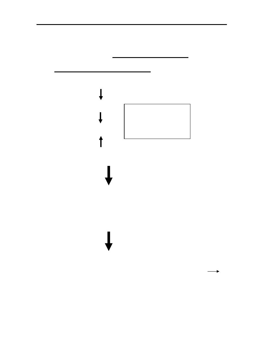
1.2 THE DESIGN PROCESS
The process of designing something is characterized as an iterative
procedure, which consists of six identifiable steps or phases:
1. Recognition of need.
2. Definition of problem.
3. Synthesis.
4. Analysis and optimization.
5. Evaluation.
6. Presentation.
Recognition of need involves the realization by someone that a
problem exists for which some corrective action should be taken. This might be
the identification of some defect in a current machine design by an engineer or the
perception of anew product marketing opportunity by a sales person.
Definition of the problem involves a thorough specification of the
item to be designed. This specification includes physical and functional
characteristics, cost, quality, and operating performance. Synthesis and analysis
are closely related and highly iterative in the design process.
A certain component or subsystem of the over all system is
conceptualized by the designer, subjected to analysis improve through this
analysis procedure and redesigned. The process is repeated until the design has
been optimized with in the constraints imposed on the designer. The components
and subsystems are synthesized into the final overall system in a similar iterative
manner.
Specification
Initial
Design

3
Evaluation is concerned with measuring the specifications established in the
problem definition phase. This evaluation often requires the fabrication and
testing of a prototype model to assess operating performance, quality, reliability
and other criteria. The final phase in the design process is the presentation of the
design. This includes documentation of the design by means of drawings, material
specifications, assembly lists, and so on .Essentially, the documentation requires
that a design data base be created.
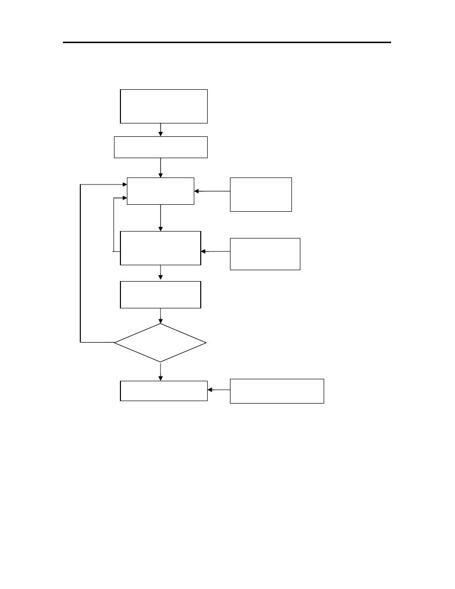
Engineering design has traditionally been accomplished on drawing
boards with the design being documented in the form of detailed engineering
drawing. Mechanical design includes the drawing of the complete product as well
as its components and subassemblies, and the tools and fixture required to
manufacture the product figure (1.1) illustrates the basic steps in the design
process indicating its iterative nature.
Electrical design is concerned with the preparation of circuit diagrams,
specification of electronic components and soon, similar manual documentation is
required in other engineering design fields (structural design, aircraft design,
chemical engineering design etc.). In each engineering discipline, the approach
has traditionally been to synthesize a preliminary design manually and then to
subject that design to same form of analysis. The analysis may involve
sophisticated engineering calculations or it may involve a very subjective
judgment of the aesthete appeal possessed by the design .the analysis procedure
identifies certain improvements that can be made in the design. As stated
previously, the process is iterative process in that it is time consuming many
engineering labor hours are required to complete the design project.
4
Figure (1.1): The general design process.
Recognition of
need
Problem definition
Synthesis
Analysis and
optimization
Evaluate Design
Presentation
Automated drafting
Engineering
analysis
Geometric
modeling
Satisfy
Specification
No
Yes

5
1.3 THE PRODUCT CYCLE AND CAD/CAM
CAD/CAM is a term which means computer aided design and
computer-aided manufacturing. It is the technologies concerned with the use of
digital computers perform certain functions in design and production. This
technology is moving in the direction of greater integration of design and
manufacturing, two activities which have traditionally been treated as distinct and
separate functions in a production firm.
CAD
(Computer Aided Design): can be defined as the use of computer systems
as assist in the creation, modification, analysis, or optimization of a design
CAM
(Computer Aided Manufacturing): can be defined as the use of computer
systems to plan, mange, and control the operations of a manufacturing
plant through either direct or indirect computer interface with the plants
production resources.
CAD/CAM:
is concerned with the application of computers to the manufacture
of engineering components starting from the drawing office, to the
production department, to the machine assembly shops, to the quality
control department, right to the finished parts store.
6
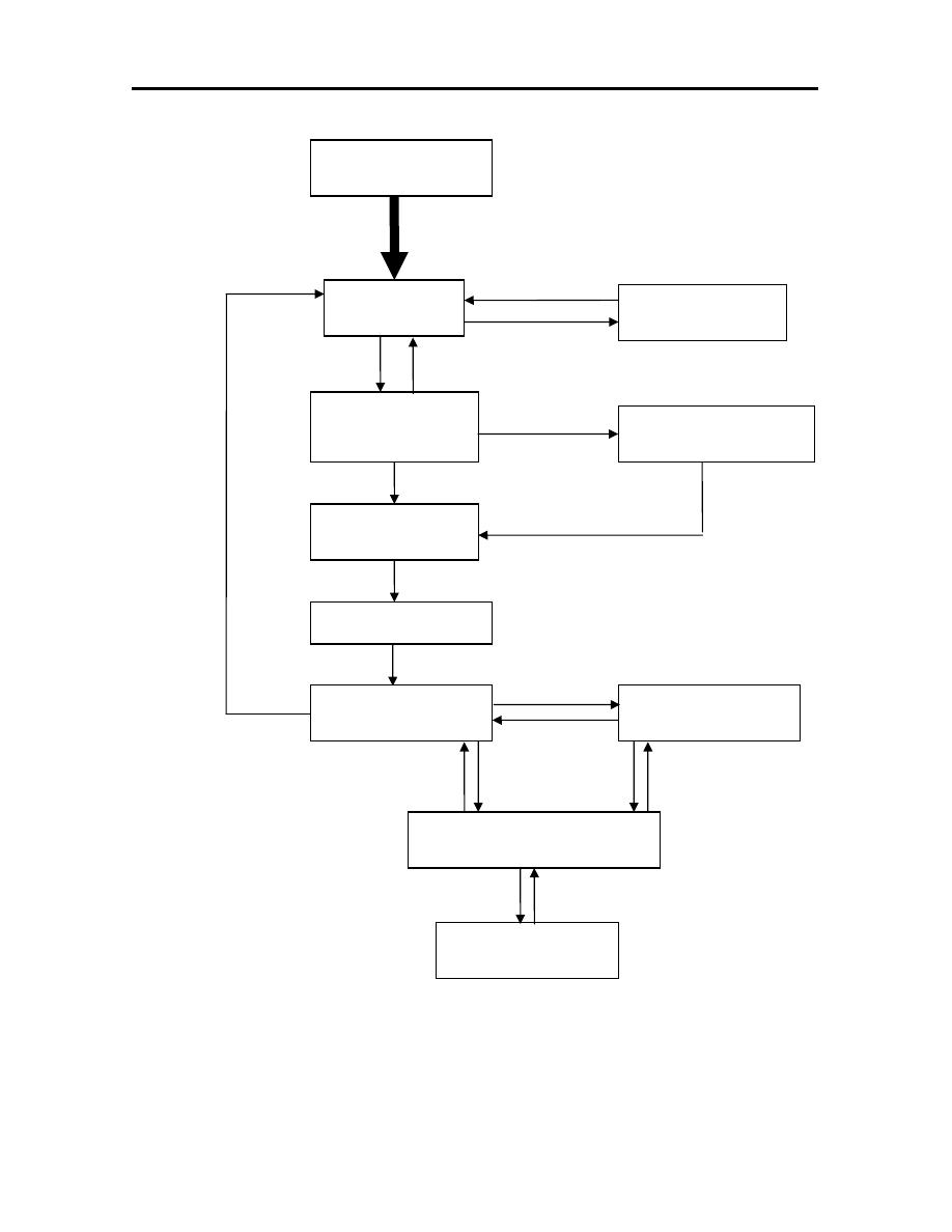
Figure (1.2): The product cycle.
Factory Specific
Customer
Design
Process
Planning
Scheduling
Stock control
Inspection
Fabrication
Test
Sales
Customer

7
From this diagram it appears that each of these activities needs to altered
or modified according to the feedback from other activities which are interacting
with it. The fast and efficient means are needed for:
1. Producing product design (geometry, loads, appearance).
2. Predicting product behavior (simulation).
3. Process planning (material, tool, and machine sequence).
4. Scheduling of machine.
5. Product fabrication (machining, forming, assembly).
6. Product inspection (in process, past process).
7. Material handling (raw material, semi finish, finish tools).
8. Marketing (cost, sale, price sale, service after sale).
9. Information handling and exchange.
The CAD include (1 and 2) while CAM include (3 to 9).
Computer
is a power full and fast tool for performing, computing, is
the right means to use for improving the efficiency of production activities. The
main benefits of computer in industry include:
1. To increase the productivity of the designer, This is accomplished by
helping the designer to visualize the product and it is component
subassemblies and parts: and by reducing the time required in synthesizing,
analyzing, and documenting the design. This productivity improvement
translates not only into lower design cost but also into shorter project
completion times.

8
2. To improve the quality of design, A CAD system permits a more thorough
engineering analysis and a larger number of design alternatives can be
investigated. Design errors are also reduced through the greater accuracy
provided by the system. These factors lead to a better design.
3. To improve documentations, use of a CAD system provides better
engineering drawings, more standardization in the drawings, better
documentation of the design, or fewer drawing errors, and greater legibility.
4- To create a data base for manufacturing, In the process of creating the
documentation for the product design (geometries and dimension of the
product and it is components, material specifications for components, bill of
materials, etc…..), much of the required data base to manufacture the product
is also created.
9
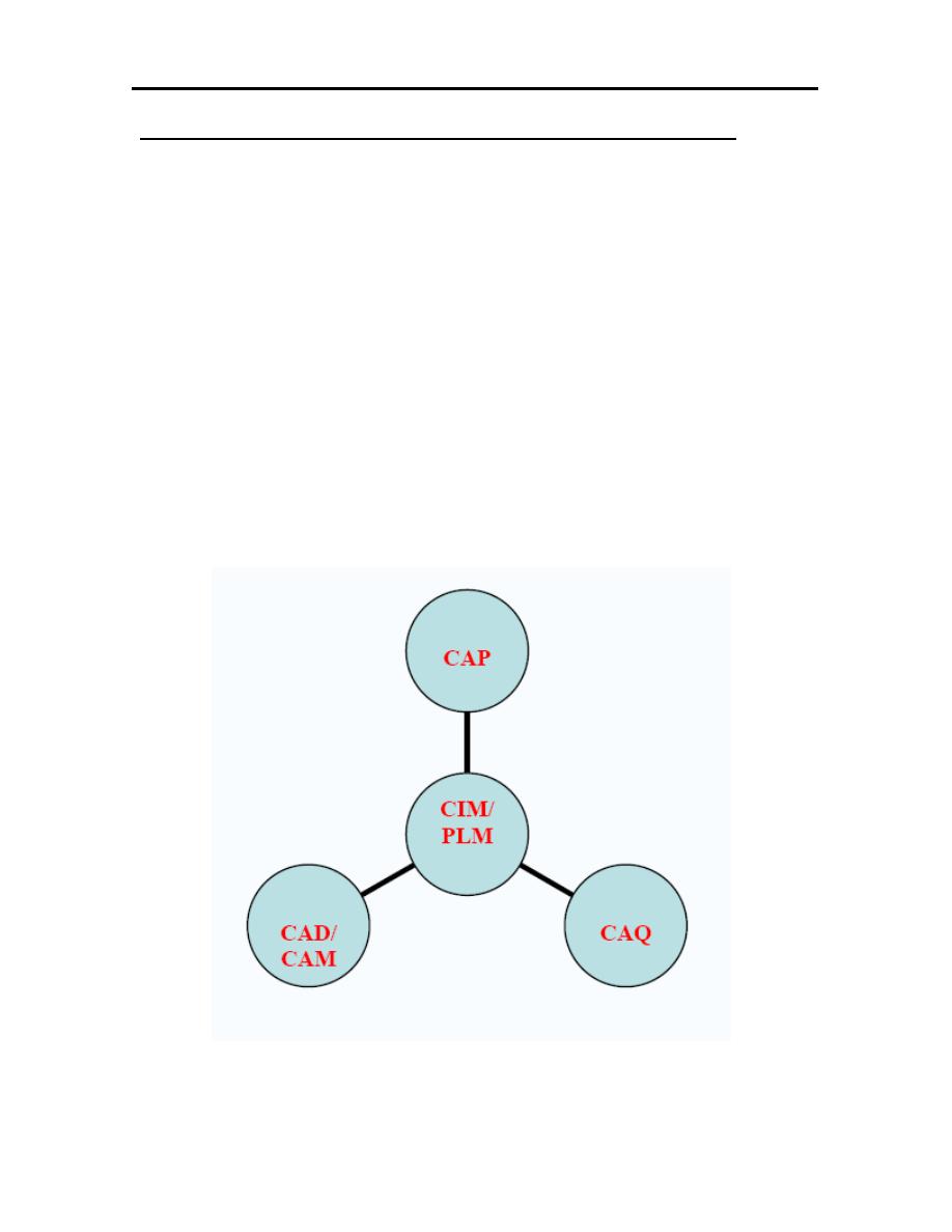
COMPUTER INTEGRATED MANUFACTURE (CIM)
Is that all the individual functions of design and manufacture are
computerized and these function are tied together through a central data base
system, that is shred among all department and activities.
Computer-integrated manufacturing (CIM) is manufacturing supported by
computers. It is the total integration of Computer Aided Design / Manufacturing
and also business operations and databases. This term has generally been replaced
by the wide field of PLM – Product Lifecycle Management. Some components of
CIM are: CAD, CAP (Computer Aided Planning), CAQ (Computer Aided Quality
Assurance), CAM (Computer aided manufacturing).
Figure (1.3): CIM diagram.

10
1.5 BENEFITS OF CAD/CAM
1. Reduce the number of steps involved in the design process.
2. Make each design step much easier and less tedious for the designer to
perform.
3. Make better decisions and will reduce the possibility of having errors.
4. The designer arrives at an optimal solution.
5. Scheduling of components and tools through manufacturing is much easier.
6. Reduce delivery time of products.
7. The working capital required by company is reduced.
8. All information is stored in the computer in stead of on paper.
1.6 APPLICATION OF CAD/CAM
1. Study of molecular structure in chemistry.
2. Medical research.
3. Aircraft flight simulation.
4. Structure design in aircraft.
5. Ship building.
6. Automobile industries.
7. Town planning.
8. Integrated circuits and printed circuit board design.
9. Mesh data preparation for finite element analysis.

11
CHAPTER TWO
COMPUTER SYSTEM
2.1 DIGITAL COMPUTER SYSTEM
Computers are now in common use in both scientific and commercial
fields. The digital computer is a major and central component of CAD/CAM
systems, so it is essential to be familiar with the technology of the digital
computer and the principle on which it works.
The modern digital computer
is an electronic machine that can
perform mathematical logical calculations and data processing functions in
accordance with a predetermined program of instructions.
The computer system consist of the hardware and software to perform
the specialized design function required by the particular user firm, the hardware
typically includes the computer, one or more graphics display terminals,
keyboard, and other peripheral equipment.
The software consists of the computer programs and instructions to
implement computer graphics on the system plus application program to facilitate
the engineering functions of the user company. Examples of these application
programs include stress-strain analysis of components, dynamic response of
mechanism, heat transfer calculations, and numerical control pant programming.
12
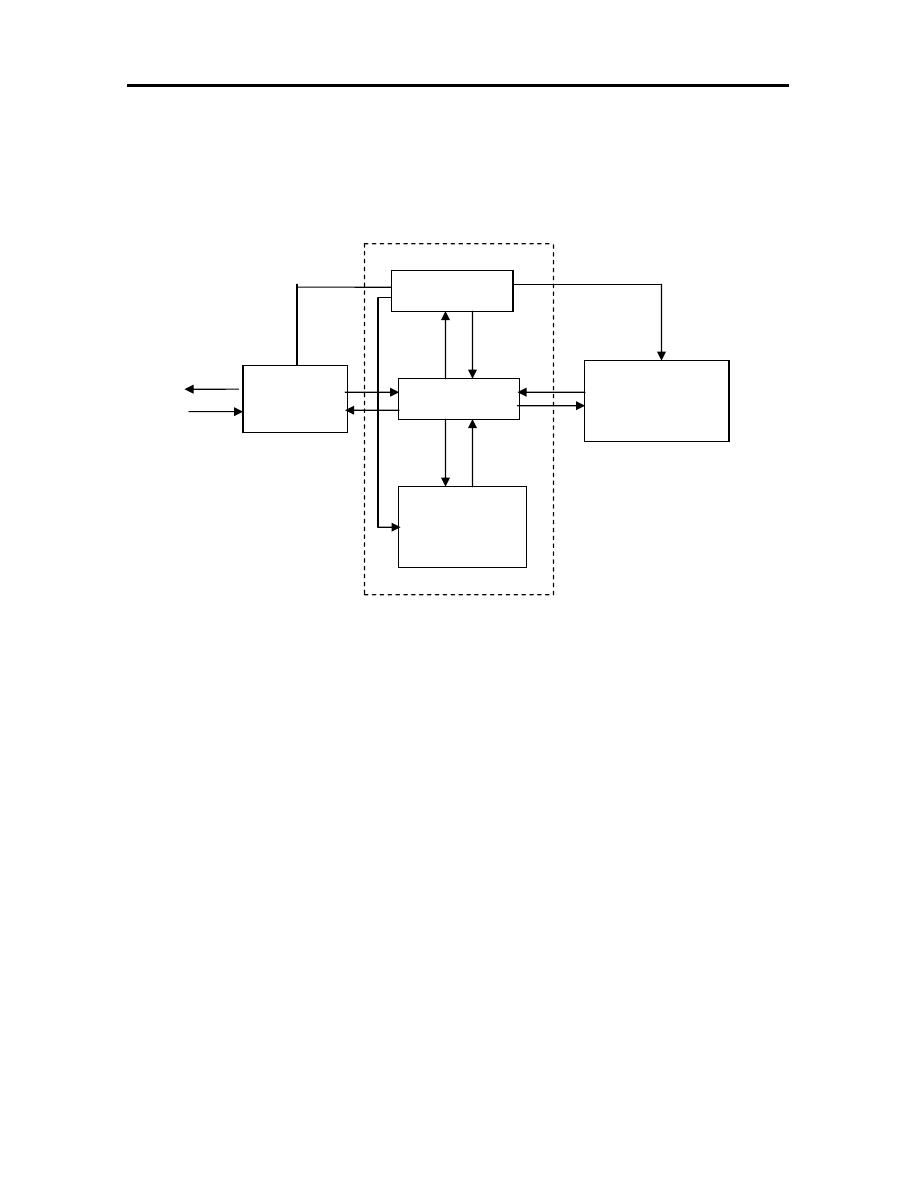
There are three basic hardware components of a general purpose
digital computer as shown in figure (2.1):
Figure (2.1): Computer System.
1. Central processing unit (CPU):The central processing unit is often
considered to consist of two subsections that:
a. Control unit: the control unit coordinates the operations of all the other
components. It control the input and output of information between the
computer and the outside world through the input/output section,
synchronizes the transfer of signals between the various sections of the
computer and commands the other section in the performance of their
function.
Controller
Memory
Arithmetic
Logic unit
Mass
storage unit
I/O unit
Output
Input
CPU

13
b. Arithmetic Logic unit: the arithmetic logic unit carries out the arithmetic
and logic manipulations of data. It adds, subtracts, multiplies, divides and
compares number according to programmed instructions.
2. Memory: the memory of the computer is the storage unit. The data stored
in this section are arranged in the form of words which can be transferred to
the arithmetic logic unit or input/output section for processing. In general
the memory classified into main and auxiliary memory.
3. Input/Output section: the input/output provides the means for the
computer to communicate with the external world. This communication is
accomplished through peripheral equipment such as printers, monitors,
keyboard, mouse…etc.
2.2 DATA REPRESENTATION
Information is handled within the computer by electrical components such
as transistors, integrated circuits, semi conductors and wires, all of which can only
indicate two states or conditions.
The binary number system is thus particularly suitable for
mathematically representation the two states possible. The binary number system
is based on the number (two) and involves only two digits zero (0) and one (1).
The meaning of successive digits in the binary system is based on the number (2)
raised to successive powers.

14
The first digit is 2
0
The second digit is 2
1
The third digit is 2
2
And so forth
Binary
Decimal
0000
0
0001
1
0010
2
0011
3
0100
4
0101
5
0110
6
0111
7
1000
8
1001
9
Example-1: Convert the binary number 11010011 into decimal one.
11010011=1x2
0
+1x2
1
+0x2
2
+0x2
3
+1x2
4
+0x2
5
+1x2
6
+1x2
7
=211
A part from the decimal and binary system, the octal and hexadecimal
number system is in common use in computers. The octal number system is based
on the number eight and involves the eight digits, zero (0) to seven (7), where as
the hexadecimal number system is based on the number sixteen and involves the
sixteen digits, zero (0) to nine (9) and A to F which represent 10 to 15.

15
Decimal
Binary
Octal
Hexadecimal
0
0
0
0
1
0001
1
1
2
0010
2
2
3
0011
3
3
4
0100
4
4
5
0101
5
5
6
0110
6
6
7
0111
7
7
8
1000
10
8
9
1001
11
9
10
1010
12
A
11
1011
13
B
12
1100
14
C
13
1101
15
D
14
1110
16
E
15
1111
17
F

16
Example-2: Convert the binary number 10111 into decimal, octal and
hexadecimal numbers.
1. To decimal number:
10111=1x2
0
+1x2
1
+1x2
2
+0x2
3
+1x2
4
= 23.
2. To octal number: (Split into groups of three binary digits) 010111=
27
3. To hexadecimal number: (Split into groups of four binary digits)
00010111= 17
HW
1. Determine the binary, octal and hexadecimal numbers equivalent to
decimal numbers (25, 90, and 1990).
2. Determine the binary, octal and decimal numbers equivalent to
hexadecimal numbers (A53C, 3D5).
3. Convert the Octal number (57011) into hexadecimal number.

17
2.3 PROGRAMMING LANGUAGE
In general there are three basic categories of computer programming
language:
1. Machine Language. Low level Language.
2. Assembly Language.
3. High level language such as:
FORTRAN, BASIC, PASCAL and COBOL………etc.
Example-3: using high level language (BASIC) to draw a line from point (X
1
,Y
1
)
to point (X
2
,Y
2
).
10 SCREEN 0: CLS
20 INPUT “from point”; X
1
,Y
1
30 INPUT “from point”; X
2
,Y
2
40 SCREEN 1: CLS
50 FOR Y= Y
1
To Y
2
60 A= ((X
2
-X
1
)*(Y-Y
1
))/(Y
2
-Y
1
)
70 X= A+X
1
80 PSET (X,Y)
90 NEXT Y

18
Example-4: Draw a circle according to it is center (150,100) and radius R using
BASIC Language.
10 SCREEN 0 : CLS
20 INPUT “Radius”; R
30 SCREEN 1 : CLS
40 PI = 3.141569
50 FOR TH = 0 TO 360
60 X = 150 + R*COS(TH*PI/180)
70 Y = 100 + R*SIN(TH*PI/180)
80 PSET (X,Y)
90 NEXT TH

19
CHAPTER THREE
GEOMETRICAL TRANSFORMATIONS
3.1 INTRODUCTION
Many of the editing features involve transformations of the graphics
elements or cell composed of the elements or even the entire model. In this
chapter we begin with a brief mathematical review of matrix algebra and then
discuss
the
mathematic
of
these
transformations.
Two
dimensional
transformations are considered, first to illustrate concepts. And deal with three
dimensions. There are several common transformations used in computer graphics
such as:
1. Scaling.
2. Reflection.
3. Rotation.
4. Translation.
3.2 MATRICES
A matrix is a rectangular array of numbers (which can be viewed as a
row of vectors) which is extensively used in computer graphics since it gives us
very compact notations. A general matrix will be represented by an upper case
letter:
=
33
32
31
23
22
21
13
12
11
a
a
a
a
a
a
a
a
a
A

20
Figure (3.1): Matrix multiplication.
The element on the ith row and jth column is denoted by aij. Note that
we start indexing at 1, where as C indexes arrays from 0 - beware! A matrix is
said to be of dimension n by m (written n x m) if it has n rows and m columns.
Matrix multiplication is more complex. Given two matrices, A and B if we want
to multiply B by A (that is form AB) then if A is (n x m), B must be (m x p). This
produces a result, C = AB, which is (n x p), with elements cij =
∑
=
m
1
k
kj
ik
b
a
, that is
the i; jth element of C is the ith row of A dot product with the jth column of B.
Note that matrix multiplication is not commutative, indeed in this case we cannot
multiply BA, since the sizes are wrong..
Matrix multiplication distributes over addition, that is A(B + C) = AB
+ AC, and there is an identity matrix for multiplication, denoted I, which is square
and has ones on the diagonal with zeros everywhere else. The transpose of a
matrix, A, which is either denoted A
T
or A
/
is obtained by swapping the rows and
columns of the matrix. Thus:
=
′
⇒
=
23
13
22
12
21
11
23
22
21
13
12
11
a
a
a
a
a
a
A
a
a
a
a
a
a
A
If we consider a (n x1) matrix (that is a column vector, s) then it
transpose s
/
is a (1 x n) matrix (which we would call a row vector)
.
21
3.3 Mathematical elements in 2-D graphics
This section considers some of the transformations that are applied to 2-D
graphics primitives and objects. This section uses many of the results that were
shown above for matrices.
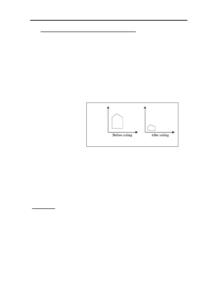
1. Scaling.
The scaling of an element is used to enlarge it or reduce its size, scaling is
the simple stretching of the object, generally about the origin. Given a point r and
a scaling matrix S, where
:
=
′
′
=
′
Y
X
].
S
[
Y
X
]
P
].[
S
[
]
P
[
=
y
x
S
0
0
S
S
Figure (3.2): 2-D Scaling.
Where S
x
is the x-axis scaling and S
y
is the y-axis scaling the location of the new
point can be written r
`
= rS. If S
x
= S
y
= S the scaling is said to be uniform and r
`
=
rS, otherwise the scaling is called differential. An example is shown in Figure
(3.2).
Example-1: Apply scaling by a factor 2.For the line defined by the points A(1,1)
and B(3,2).
=
4
2
6
2
2
1
3
1
2
0
0
2
The line scaled to
A
′
(2,2) and
B
′
(6,4).
22
Commands in Auto CAD:
Scale
↵
or
Select objects: “use mouse left click sign the objects”
↵
Specify base point:
Specify scale factor or [Reference]: ….
↵
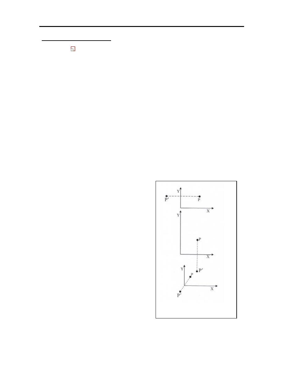
2. Reflection or mirror:
Reflection or mirror is a transformation, which allows a copy of the object
to be displayed while the object is reflected about a line or plane.
=
′
′
=
′
Y
X
].
F
[
Y
X
]
P
].[
F
[
]
P
[
a. about Y-axis
−
=
=
′
′
1
0
0
1
F
Y
X
].
F
[
Y
X
b. about X-axis.
−
=
=
′
′
1
0
0
1
F
Y
X
].
F
[
Y
X
c. about origin
−
−
=
=
′
′
1
0
0
1
F
Y
X
].
F
[
Y
X
Figure (3.3): 2-D Reflection
23
Commands in Auto CAD:
Mirror
↵
or
Select objects: “use mouse left click sign the objects”
↵
Specify first point of mirror line:
Specify second point of mirror line:
↵
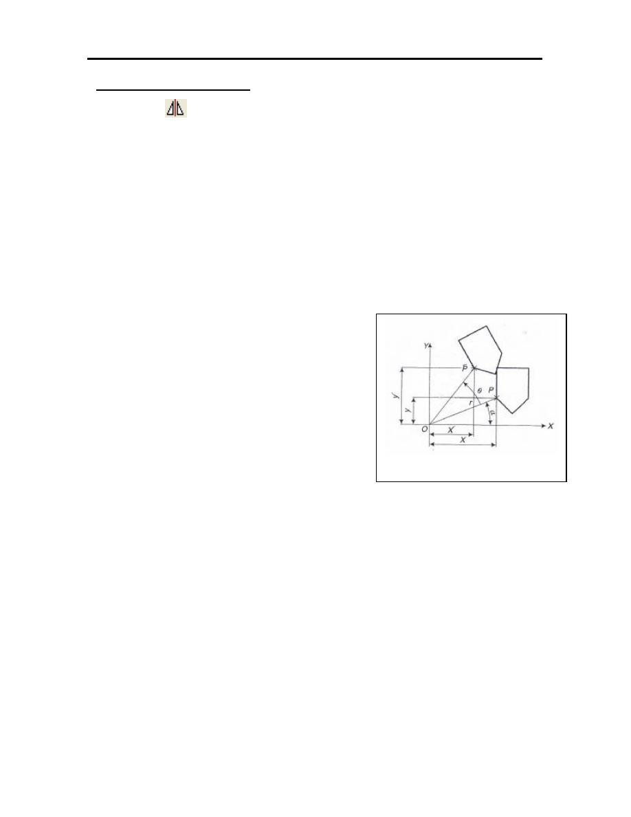
3. Rotation
In this transformation the points of the objects are rotate about the origin
by an angle θ. The final position and orientation of a geometric entity is described
by the angle of rotation and the base point about which the rotation, the general
formula is given by:
=
′
′
Y
X
].
R
[
Y
X
From figure (3.4), the general position is:
X=rcosα
Y=rsinα
The new position
is specified by:
−
=
′
′
+
=
+
=
+
=
′
−
=
−
=
+
=
′
Y
X
.
cos
sin
sin
cos
Y
X
cos
Y
sin
X
sin
cos
r
cos
sin
r
)
(
sin
r
Y
sin
Y
cos
X
sin
sin
r
cos
cos
r
)
rcos(
X
θ
θ
θ
θ
θ
θ
α
θ
α
θ
θ
α
θ
θ
α
θ
α
θ
θ
α
Where,
−
=
θ
θ
θ
θ
cos
sin
sin
cos
]
R
[
Figure (3.4): 2-D Rotation.

24
Note that positive θ implies an anti-clockwise rotation. It is a simple
exercise to show, using simple trigonometry, that R is indeed a matrix which
rotates points by θ.
Example-2: Rotate the line
2
1
4
2
about the origin by 30º CCW.
=
−
732
.
2
866
.
1
464
.
2
232
.
1
2
1
4
2
30
cos
30
sin
30
sin
30
cos
Commands in Auto CAD:
Rotate
↵
or
Select objects: “use mouse left click sign the objects”
↵
Specify base point:
Specify angle rotation or [Reference]: …..
↵
4. Translation
Involves moving the geometric entity from one location to another, the
new entity is parallel at all the points to the old entity. The general formula in
matrix notation is:
)
t
,
t
(
T
Y
X
].
T
[
Y
X
y
x
=
+
=
′
′
Where t
x
is the unit translates in X-axis and t
y
is the unit translates in Y-axis.
Figure (3.5): 2-D Translation.
Before translation
After translation

25
Example-3: Translate the line defined by (4,5) and (3,7) by 1 unit in X-direction
and 2 unit in Y-direction.
+
=
′
′
Y
X
].
T
[
Y
X
=
+
9
7
4
5
7
5
3
4
2
2
1
1
Commands in Auto CAD:
Move
↵
or
Select objects: “use mouse left click sign the objects”
↵
Specify base point of displacement:
Specify second point of displacement or<use first reference as displacement>:
↵
5. Concatenation of transformation
Many a times it becomes necessary to combine the individual transformations as
shown above in order to achieve the required results. In such cases, the combined
transformation matrix can be obtained by multiplying the respective
transformation matrices. However, care must be taken to see that the order of the
matrix multiplication be done in the same as that of the transformations as
follows:
[T]=[T
n
][T
n-1
][T
n-2
]……….[T
3
][T
2
][T
1
].

26
3.4 HOMOGENEOUS COORDINATES
Representing 2D coordinates in terms of vectors with 2 components
turns out to be rather awkward when it come to the sort of manipulation that needs
to be carried out for computer graphics.
Homogeneous coordinates allow us to treat all transformations in the
same way, as matrix multiplications. The consequence is that our 2-vectors
become extended to 3-vectors, with a resulting increase in storage and processing.
Homogeneous coordinates mean that we represent a point (x; y) by the extended
triple (x; y; w). In general w should be non-zero. The normalized homogeneous
coordinates are given by (x/w; y/w; 1) where (x/w; y/w) are the Cartesian
coordinates of the point. Note in homogeneous coordinates (x; y; w) is the same
as (x/w; y/w; 1) as is (ax; ay; aw) where a can be any real number. Points with
w = 0 are called points at infinity, and are not frequently used.
Vector triples usually represent points in 3D space, however here we are
using them to represent points in 2D space, so what is going on. Well we are using
a bit of mathematical trickery to make life easy for ourselves. If you like then you
can think of 2D space corresponding to plane w = 1.
Now in homogeneous coordinates the transformations can be given as:
=
′
′
1
Y
X
1
0
0
0
S
0
0
0
S
1
Y
X
Scaling
Y
X

27
=
′
′
θ
θ
θ
−
θ
=
′
′
−
−
=
′
′
−
=
′
′
−
−
=
′
′
−
1
Y
X
1
0
0
t
1
0
t
0
1
1
Y
X
n
Translatio
1
Y
X
1
0
0
0
cos
sin
0
sin
cos
1
Y
X
Rotation
1
Y
X
1
0
0
0
1
0
0
0
1
1
Y
X
origin
the
about
1
Y
X
1
0
0
0
1
0
0
0
1
1
Y
X
axis
X
about
1
Y
X
1
0
0
0
1
0
0
0
1
1
Y
X
axis
Y
about
flection
Re
Y
X
28
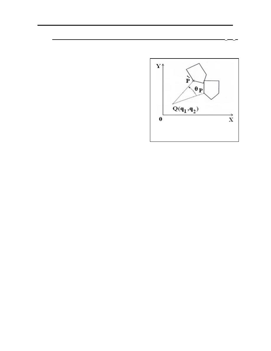
3.5 2-D ROTATION ABOUT AN ARBITRARY POINT Q(q
1
,q
2
)
If we wanted to rotate an object about any arbitrary point (Q), by angle
(θ) this can easily be achieved by:
1. Translate the object by (-Q),
−
−
=
1
0
0
q
1
0
q
0
1
]
T
[
2
1
1
2. Rotate object by angle (θ),
θ
θ
θ
−
θ
=
1
0
0
0
cos
sin
0
sin
cos
]
T
[
2
3. Translate the object back to the original position by (Q).
=
1
0
0
q
1
0
q
0
1
]
3
T
[
2
1
One of the big advantages of homogeneous coordinates is that transformations can
be very easily combined. All that is required is multiplication of the
transformation matrices. This makes otherwise complex transformations very easy
to compute. For instance if we wanted to rotate an object about some point, Q, this
can easily be achieved by:
]
T
[
]
T
][
T
[
]
T
[
1
2
3
=
−
−
θ
θ
θ
−
θ
=
1
0
0
q
1
0
q
0
1
1
0
0
0
cos
sin
0
sin
cos
1
0
0
q
1
0
q
0
1
]
T
[
2
1
2
1
θ
−
θ
−
θ
θ
θ
+
θ
−
θ
−
θ
=
1
0
0
sin
q
)
cos
1
(
q
cos
sin
sin
q
)
cos
1
(
q
sin
cos
]
T
[
1
2
2
1
Figure (3.6): Rotation about an
arbitrary point
29
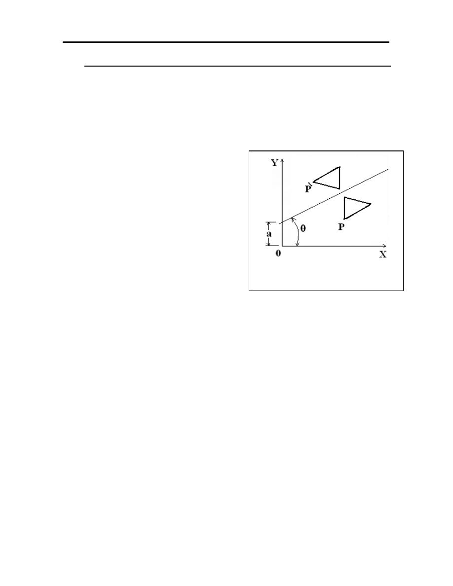
3.6 REFLECTION ABOUT AN ARBITRARY AXIS (Y =a+bX)
The transformations given earlier for reflection are about origin or about
the coordinate’s axes. However sometimes it may be necessary to get the
reflection about an arbitrary line as shown in figure (3.7). To derive the necessary
transformation matrix, the following complex procedure is required:
1. Translate the mirror line along the
Y-axis such that the line passes
through the origin (o):
−
=
1
0
0
a
1
0
0
0
1
]
T
[
1
2. Rotate the mirror line such that it
coincide with the X-axis:
θ
θ
−
θ
θ
=
1
0
0
0
cos
sin
0
sin
cos
]
T
[
2
3. Mirror the object through the X-axis:
−
=
1
0
0
0
1
0
0
0
1
]
T
[
3
4. Rotate the mirror line back to the original angle with the X-axis:
θ
θ
θ
−
θ
=
1
0
0
0
cos
sin
0
sin
cos
]
T
[
4
Figure (3.7): Reflection about an
arbitrary axis.

30
5. Translate the mirror line along the Y-axis back to the original position:
=
1
0
0
a
1
0
0
0
1
]
T
[
5
The required transformation matrix is given by:
[T]=[T
5
][T
4
][T
3
][T
2
][T
1
]
+
θ
θ
−
θ
θ
−
θ
θ
=
−
θ
θ
−
θ
θ
−
θ
θ
θ
−
θ
=
1
0
0
)
1
2
(cos
a
2
cos
2
sin
2
sin
a
2
sin
2
cos
]
T
[
1
0
0
a
1
0
0
0
1
1
0
0
0
cos
sin
0
sin
cos
1
0
0
0
1
0
0
0
1
1
0
0
0
cos
sin
0
sin
cos
1
0
0
a
1
0
0
0
1
]
T
[

31
Example-4: Given the line (5,7) and (9,9)
a- Translate the line through (-6,3.3).
b- Rotate the line through 35
°
about the origin.
c- Rotate the line about its end point (5,7) by 40
°
CW.
Solution:
a-
=
′
′
1
Y
X
1
0
0
t
1
0
t
0
1
1
Y
X
Y
X
−
=
−
=
′
′
1
1
3
.
12
3
.
10
3
1
1
1
9
7
9
5
1
0
0
3
.
3
1
0
6
0
1
1
Y
X
b-
θ
θ
θ
−
θ
=
′
′
1
Y
X
1
0
0
0
cos
sin
0
sin
cos
1
Y
X
=
−
=
′
′
1
1
535
.
12
6
.
8
21
.
2
081
.
0
1
1
9
7
9
5
1
0
0
0
35
cos
35
sin
0
35
sin
35
cos
1
Y
X
C-1. Translate the object by (-Q),
−
−
=
−
−
=
1
0
0
7
1
0
5
0
1
1
0
0
q
1
0
q
0
1
]
T
[
2
1
1
2. Rotate object by angle (θ),
−
−
−
−
−
=
θ
θ
θ
−
θ
=
1
0
0
0
40
cos
40
sin
0
40
sin
40
cos
1
0
0
0
cos
sin
0
sin
cos
]
T
[
2

32
3. Translate the object back to the original position by (Q).
=
=
1
0
0
7
1
0
5
0
1
1
0
0
q
1
0
q
0
1
]
3
T
[
2
1
Thus:
=
−
−
−
−
−
−
−
=
′
′
1
1
96
.
5
7
35
.
9
5
1
1
9
7
9
5
1
0
0
7
1
0
5
0
1
1
0
0
0
40
cos
40
sin
0
40
sin
40
cos
1
0
0
7
1
0
5
0
1
1
Y
X
Example-5: Reflect the triangle (20,40), (50,50) and (30,60) about the arbitrary
axis { Y= 15- (15/10)X}.
Solution:
1. Translate the mirror line along the Y-axis such that the line passes through
the origin (o):
−
=
1
0
0
15
1
0
0
0
1
]
T
[
1
2. Rotate the mirror line such that it coincide with the X-axis:
−
−
−
−
−
=
θ
θ
−
θ
θ
=
−
=
−
=
θ
−
1
0
0
0
3
.
56
cos
3
.
56
sin
0
3
.
56
sin
3
.
56
cos
1
0
0
0
cos
sin
0
sin
cos
]
T
[
3
.
56
)
10
/
15
(
tan
2
1
o

33
3. Mirror the object through the X-axis:
−
=
1
0
0
0
1
0
0
0
1
]
T
[
3
4. Rotate the mirror line back to the original angle with the X-axis:
−
−
−
−
−
=
θ
θ
θ
−
θ
=
1
0
0
0
3
.
56
cos
3
.
56
sin
0
3
.
56
sin
3
.
56
cos
1
0
0
0
cos
sin
0
sin
cos
]
T
[
4
5. Translate the mirror line along the Y-axis back to the original position:
=
=
1
0
0
15
1
0
0
0
1
1
0
0
a
1
0
0
0
1
]
T
[
5
The required transformation matrix is given by:
[T]=[T
5
][T
4
][T
3
][T
2
][T
1
]
−
−
−
−
−
−
−
−
−
−
−
−
=
1
0
0
15
1
0
0
0
1
1
0
0
0
3
.
56
cos
3
.
56
sin
0
3
.
56
sin
3
.
56
cos
1
0
0
0
1
0
0
0
1
1
0
0
0
3
.
56
cos
3
.
56
sin
0
3
.
56
sin
3
.
56
cos
1
0
0
15
1
0
0
0
1
]
T
[
+
−
−
−
−
−
−
−
−
=
′
′
+
−
−
−
−
−
−
−
−
=
1
1
1
60
50
40
30
50
20
1
0
0
)
1
)
3
.
56
(
2
(cos
15
)
3
.
56
(
2
cos
)
3
.
56
(
2
sin
)
3
.
56
(
2
sin
15
)
3
.
56
(
2
sin
)
3
.
56
(
2
cos
1
Y
X
1
0
0
)
1
)
3
.
56
(
2
(cos
15
)
3
.
56
(
2
cos
)
3
.
56
(
2
sin
)
3
.
56
(
2
sin
15
)
3
.
56
(
2
sin
)
3
.
56
(
2
cos
]
T
[
−
−
−
−
=
′
′
1
1
1
44
.
4
6
.
17
2
.
6
87
.
52
53
.
51
75
.
30
1
Y
X

34
Example-6: Two points, A and B, constituting a portion of a two-dimensional
shape are moved to points C and D, respectively, resulting in
transformation the original shape. List the required transformation
matrices, in proper order, that have to be applied to all the points of
the shape. The coordinates of the points are A(2,2), B(5,5), C(5,2)
and D
(7,2 + 2√3).
Solution:
To move points A and B to C and D, respectively, four steps are involved:
1. Translation the line AB from the location A to the origin, and the
transformation matrix is:
−
−
=
1
0
0
2
1
0
2
0
1
]
T
[
1
2. Rotation the line AB about Z-axis by angle and the angle is calculated>
The angle between AB and the X-axis is:
o
45
2
5
2
5
tan
1
AB
=
−
−
=
α
−
The angle between CD and the X-axis is:
o
0
6
5
7
2
)
3
2
2
(
tan
1
CD
=
−
−
+
=
β
−
The angle between the line AB and CD is 60º -45º =15º, rotate the line AB
about the Z-axis by 15º, the transformation matrix is:
−
=
1
0
0
0
15
cos
15
sin
0
15
sin
15
cos
]
T
[
2
3. Scale the line AB so that the line is the same in length as line CD:

35
4
2
)
464
.
3
(
CD
242
.
4
3
3
AB
2
2
2
2
=
+
=
=
+
=
The scaling factor is CD/AB=4/4.242=0.942
=
1
0
0
0
942
.
0
0
0
0
942
.
0
]
T
[
3
4. Translation the line AB to the location of C so that A and B will coincide
with C and D respectively. The transformation matrix is:
=
1
0
0
2
1
0
5
0
1
]
T
[
4
The equivalent transformation matrix is:
+
=
−
−
=
′
′
−
−
=
−
−
−
=
1
1
3
2
2
2
7
5
1
1
5
2
5
2
1
0
0
31
.
0
91
.
0
24
.
0
67
.
3
24
.
0
91
.
0
1
1
0
0
31
.
0
91
.
0
24
.
0
67
.
3
24
.
0
91
.
0
1
0
0
2
1
0
2
0
1
1
0
0
0
15
cos
15
sin
0
15
sin
15
cos
1
0
0
0
942
.
0
0
0
0
942
.
0
1
0
0
2
1
0
5
0
1
]
[
Y
X
T

36
3.7 Mathematical elements in 3-D graphics
1. 3-D Translation: To translate the point (X,Y,Z) to new point
)
Z
,
Y
,
X
(
′
′
′
through (t
x
, t
y
, t
z
) we use:
=
′
′
′
1
Z
Y
X
1
0
0
0
t
1
0
0
t
0
1
0
t
0
0
1
1
Z
Y
X
z
y
x
2. 3-D Reflection: An object is reflected through a plane by manipulating the
diagonal elements in 3-D matrix.
=
′
′
′
1
Z
Y
X
]
F
[
1
Z
Y
X
−
=
1
0
0
0
0
1
0
0
0
0
1
0
0
0
0
1
F
Reflection through YZ plane (around X-axis)
−
=
1
0
0
0
0
1
0
0
0
0
1
0
0
0
0
1
F
Reflection through XZ plane (around Y-axis)
−
=
1
0
0
0
0
1
0
0
0
0
1
0
0
0
0
1
F
Reflection through XY plane (around Z-axis)
3. 3-D Scaling: The diagonal terms of the general (4
×
4) transformation matrix
provide scaling:
37
=
′
′
′
1
Z
Y
X
1
0
0
0
0
S
0
0
0
0
S
0
0
0
0
S
1
Z
Y
X
z
y
x
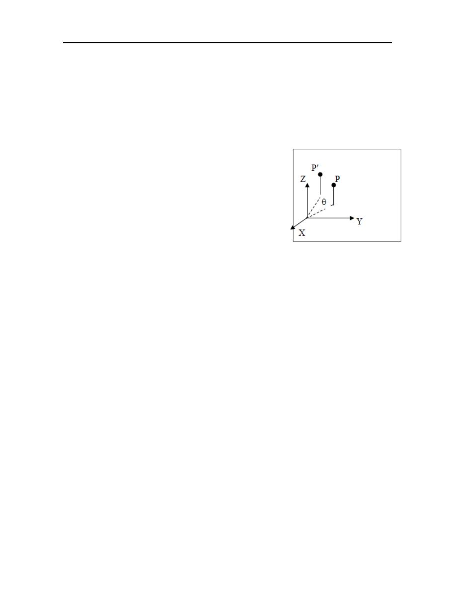
3-D Rotation:
=
′
′
′
1
Z
Y
X
]
R
[
1
Z
Y
X
The rotation transformation matrix about x-axis:
θ
θ
θ
−
θ
=
θ
1
0
0
0
0
cos
sin
0
0
sin
cos
0
0
0
0
1
)
(
R
x
The rotation transformation matrix about y-axis:
θ
θ
−
θ
θ
=
θ
1
0
0
0
0
cos
0
sin
0
0
1
0
0
sin
0
cos
)
(
R
y
The rotation transformation matrix about z-axis:
θ
θ
θ
−
θ
=
θ
1
0
0
0
0
1
0
0
0
0
cos
sin
0
0
sin
cos
)
(
R
z

38
Example-7: For a rectangular object of points (2,2,6), (8,2,6), (8,8,6), (2,8,6),
(2,2,3), (8,2,3), (8,8,3) and (2,8,3):
a- Change the scale by 3,2,1 in x,y,z respectively.
b- Reflect the object through XY plane.
c- Rotate the object around Z-axis by 20
°
.
Solution
a
-
=
′
′
′
1
Z
Y
X
1
0
0
0
0
S
0
0
0
0
S
0
0
0
0
S
1
Z
Y
X
z
y
x
=
=
′
′
′
1
1
1
1
1
1
1
1
3
3
3
3
6
6
6
6
16
16
4
4
16
16
4
4
6
24
24
6
6
24
24
6
1
1
1
1
1
1
1
1
3
3
3
3
6
6
6
6
8
8
2
2
8
8
2
2
2
8
8
2
2
8
8
2
1
0
0
0
0
1
0
0
0
0
2
0
0
0
0
3
1
Z
Y
X
b-
=
′
′
′
1
Z
Y
X
]
F
[
1
Z
Y
X
−
−
−
−
−
−
−
−
=
−
=
′
′
′
1
1
1
1
1
1
1
1
3
3
3
3
6
6
6
6
16
16
4
4
16
16
4
4
6
24
24
6
6
24
24
6
1
1
1
1
1
1
1
1
3
3
3
3
6
6
6
6
8
8
2
2
8
8
2
2
2
8
8
2
2
8
8
2
1
0
0
0
0
1
0
0
0
0
1
0
0
0
0
1
1
Z
Y
X
c-
=
′
′
′
1
Z
Y
X
]
R
[
1
Z
Y
X

39
−
−
=
−
=
′
′
′
1
1
1
1
1
1
1
1
3
3
3
3
6
6
6
6
2
.
8
25
.
10
61
.
4
56
.
2
2
.
8
25
.
10
61
.
4
56
.
2
85
.
0
78
.
4
83
.
6
19
.
1
85
.
0
78
.
4
83
.
6
19
.
1
1
1
1
1
1
1
1
1
3
3
3
3
6
6
6
6
8
8
2
2
8
8
2
2
2
8
8
2
2
8
8
2
1
0
0
0
0
1
0
0
0
0
20
cos
20
sin
0
0
20
sin
20
cos
1
Z
Y
X
40
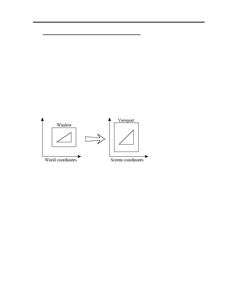
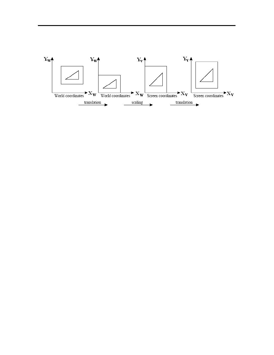
3.8 Window to viewport transformation
In general the objects and primitives represented in the application model
will be stored in world coordinates that is their size, shape, position, etc. will be
given in terms of logical units for whatever the object represent (e.g. mm, cm, m,
km or light years). Thus to display the appropriate images on the screen (or other
device) it is necessary to map from world coordinates to screen or device
coordinates. This transformation is known as the window to viewport
transformation, the mapping from the world coordinate window to the viewport
(which is given in screen coordinates).
Figure (3.8): The window to viewport transformation.
In general the window to viewport transformation will involve a scaling and
translation as in Figure (3.8), where the scaling in non-uniform (the vertical axis
has been stretched). Non uniform scaling result from the world coordinates
window and viewport having different aspect ratios. In Figure the screen window
(that is the viewport) covers only part of the screen.
The transformation is generally achieved by a translation in world
coordinates, a scaling to viewport coordinates and another translation in viewport
coordinates, which are generally composed to give a single transformation matrix.
Often the clipping of visible elements will be carried out at the same time as the
41
transformation is applied. Typically the region will be clipped in world
coordinates and then transformed.
Figure (3.9): The procedure used to transform from world coordinate window to viewport.
The required transformations are shown in Figure (3.9). If the world
coordinate window has dimensions (x
wmin
; y
wmin
) and (x
wmax
; y
wmax
), while the
viewport (or screen coordinate window) has dimensions x
Vmin
; y
Vmin
) and (x
Vmax
;
y
Vmax
), then the transformation will be given by: a translation;
−
−
=
1
0
0
Y
1
0
X
0
1
T
min
w
min
w
1
a scaling:
=
=
1
0
0
0
S
0
0
0
S
S
T
Y
X
2
and finally another translation;
=
1
0
0
Y
1
0
X
0
1
T
min
V
min
V
3
These can be combined to yield the transformation matrix:

42
min
w
max
w
min
V
max
V
y
min
w
max
w
min
V
max
V
x
min
w
y
min
V
y
min
w
x
min
V
x
wv
min
w
min
w
Y
X
min
V
min
V
wv
Y
Y
Y
Y
S
X
X
X
X
S
Where
1
0
0
Y
S
Y
S
0
X
S
X
0
S
M
1
0
0
Y
1
0
X
0
1
1
0
0
0
S
0
0
0
S
1
0
0
Y
1
0
X
0
1
M
−
−
=
−
−
=
−
−
=
−
−
=
Example: Estimate the transformation matrix required to transform the (2,2) and
(4,3) from the world coordinates to the screen coordinates at (0.5,1) and
(3,2.25).
Solution:
−
−
=
−
−
=
−
−
=
=
−
−
=
−
−
=
=
−
−
=
−
−
=
1
0
0
5
.
1
25
.
1
0
2
0
25
.
1
M
1
0
0
2
*
25
.
1
1
25
.
1
0
2
*
25
.
1
5
.
0
0
25
.
1
M
1
0
0
Y
S
Y
S
0
X
S
X
0
S
M
25
.
1
2
3
1
25
.
2
Y
Y
Y
Y
S
25
.
1
2
4
5
.
0
3
X
X
X
X
S
wv
wv
min
w
y
min
V
y
min
w
x
min
V
x
wv
min
w
max
w
min
V
max
V
y
min
w
max
w
min
V
max
V
x
43
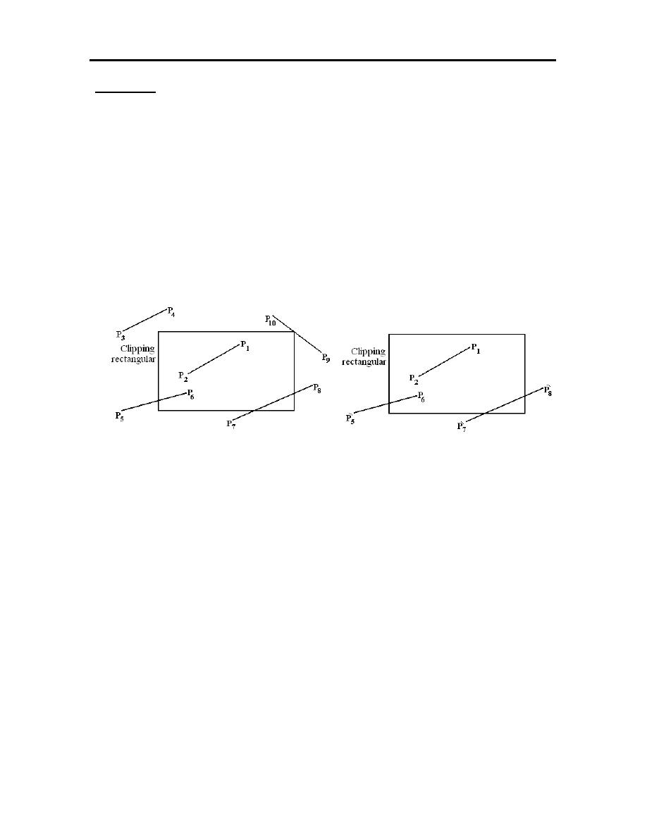
Clipping:
Clipping is a very important element in the displaying of graphical images.
This helps in discarding the part of the geometry outside the viewing window,
such that all the transformation that are to be carried out of zooming and panning
of the image on the screen are applied only on the necessary geometry.
In order to carry out the clipping operation for lines, it is necessary to know
the lines are completely inside the clipping rectangle, completely outside the
rectangle or partially inside the rectangle as shown in figure (3.10).
Figure (3.10): The clipping operation
To know whether a line is completely inside or outside the clipping
rectangle, the end points of the line can be compared with the clipping boundaries.
For example, the line P
1
P
2
is completely inside the clipping rectangle, similarly
line P
3
P
4
and P
9
P
10
are completely outside the clipping rectangle.
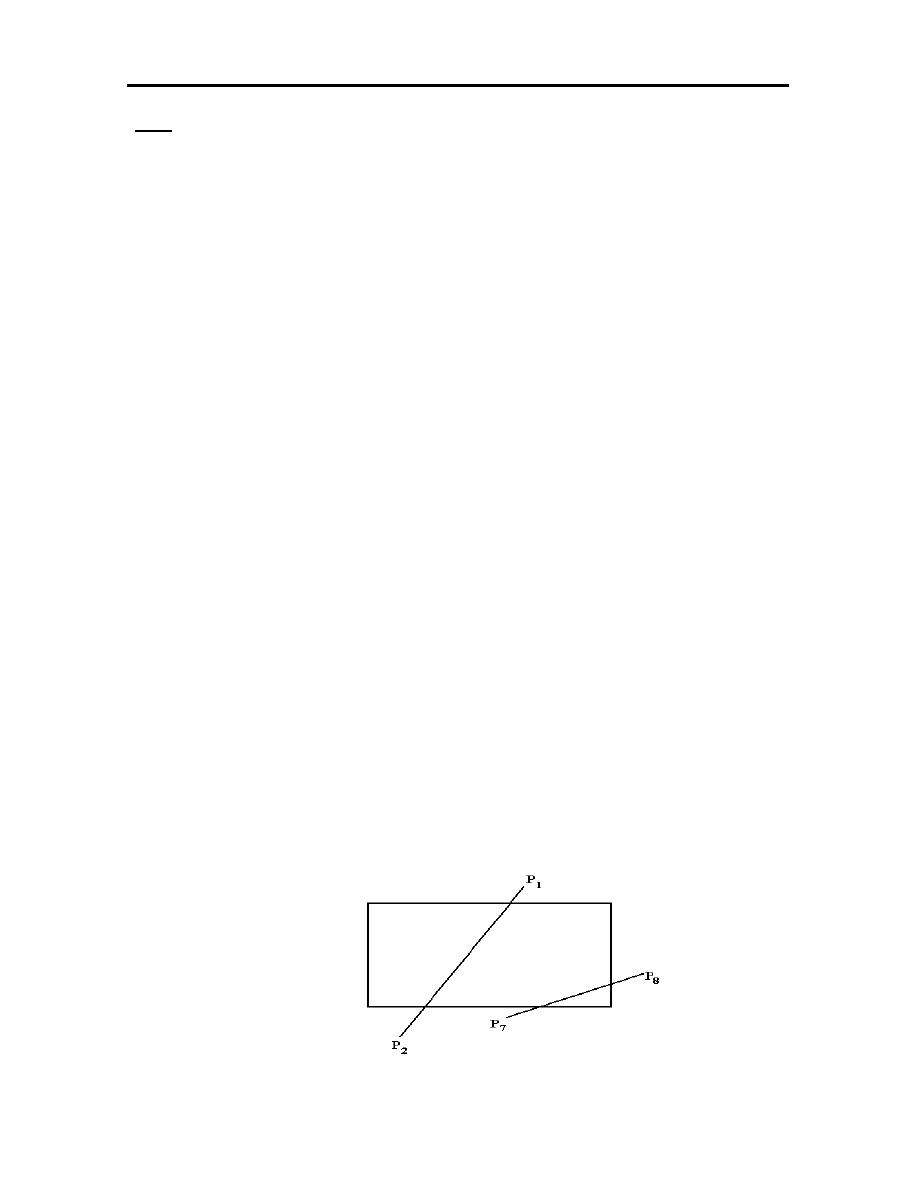
In Cohen- Sutherland clipping algorithm of 2-D, the lines are classified as
to whether they are in, out or partially in the window by doing an edge test. The
end points of the line are classified as to where they are with reference to the
window by means of a 4-digit binary code. The code is given as TBRL. The code
is identified as follows:

44
T=1 if the point is above the top of the window.
=0 otherwise.
B= 1 if the point is above the bottom of the window.
=0 otherwise.
R= 1 if the point is above the right of the window.
=0 otherwise.
L= 1 if the point is above the left of the window.
=0 otherwise.
1001
1000
1010
0001
0000
0010
0101
0100
0110
The 4-digit coding of the line end points for clipping
- The line is completely inside the window if both the end points are equal to
(0000).
- The line is completely outside the window if both the end points are not
equal to (0000) and a 1 in the same bit position for both ends.
45
HW
1. Reflect an object defined by the points (1,2), (3,5), (7,8) and (4,4) about an
arbitrary axis basses through the points (4,4) and (9,6).
2. An object is defined by the points (1,2), (6,4), (8,7) and (3,5), perform
the following transformations on it:
a. Reflect the object about an arbitrary axis defined by the points (1,2)
and (6,4).
b. Scale the object by a factors of (0.5 in X-direction and 2 in Y-
direction).
3. An object is defined by the points (5,7), (4,8) and (1,-2). Perform the
following transformation on it:
a. Rotate the object about the point (2,-1) by 35º CW.
b. Apply scaling on the object by 2 in X-direction.
4. ِِReflect the object defined by the points (2,3), (5,5), (5,7) and (2,8), about
the axis Y=3-X.
5. A cube of 10 unit length has one of its corners at the origin (0,0,0) and the
three edges along the three principle axes. If the cube is to be rotated about
the Z-axis by an angle of 30º CCW direction. Calculate the new position of
the cube.
6. Using Cohen- Sutherland clipping algorithm to test whether the line shown
inside or outside the window.

46
CHAPTER FOUR
FINITE ELEMENT METHOD
4.1 INTRODUCTION
The finite element method has developed simultaneously with the
increasing of high speed electronic digital computer and with the growing
emphasis on numerical method for engineering analysis. Although the method
was originally developed for structural analysis, the general nature of the theory
on which it is based has also made possible its successful application for solutions
of problems in other field of engineering.
The analytical solution only for desired unknown quantity at any location in
the body. Analytical solutions can be obtained only for a certain simplified
situations. For problems involves complex material properties and boundary
conditions using Finite Element Method. The process of selecting only a certain
number of discrete points in the body can be termed discretizations.
The Finite Element Method consists of five essential states:
1. Definition of the Finite Element Method mesh.
2. Selecting a displacement model.
3. Formulate the discrete equation.
4. Solving the stiffness equation.
5. Determining element stresses and strains.
47
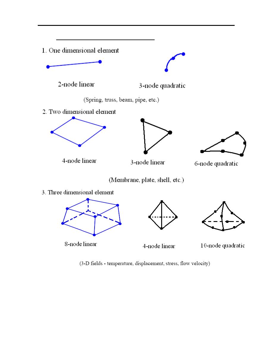
4.2
TYPES OF FINITE ELEMENT
48
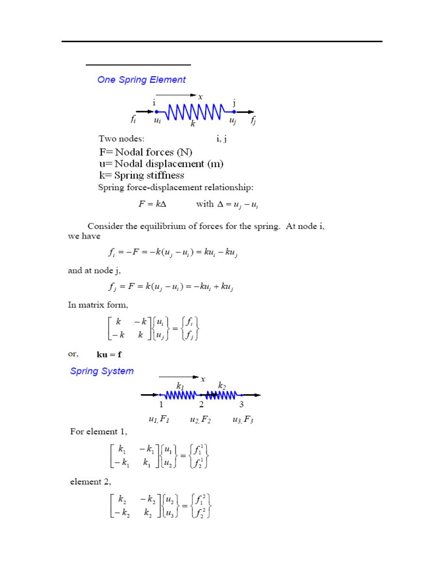
4. 3 SPRING ELEMENT
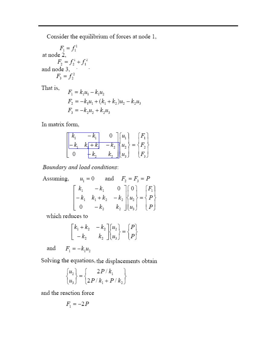
49
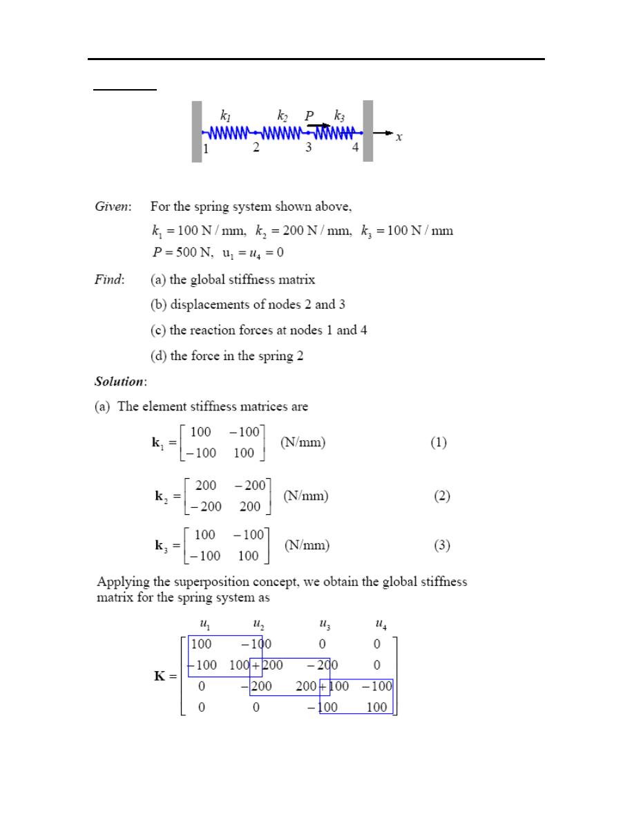
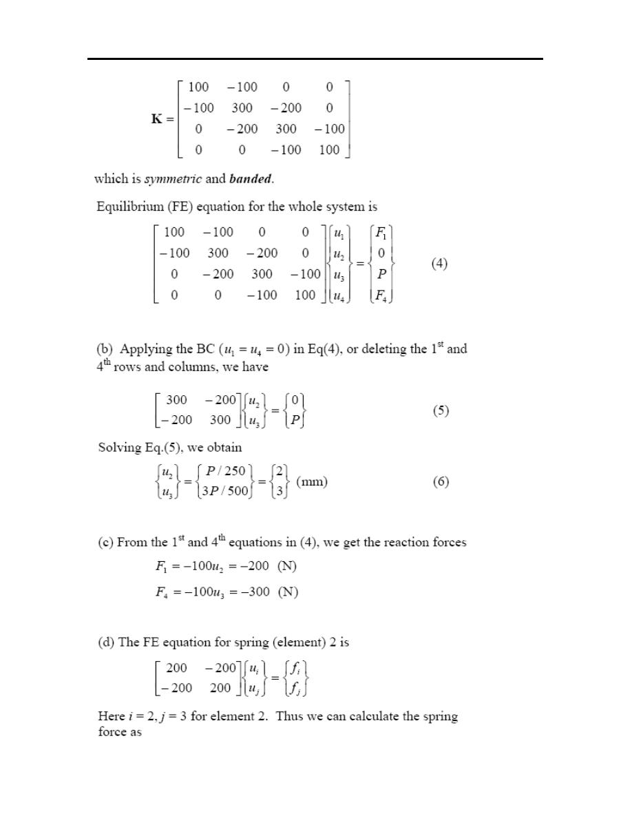
50
Example-1
51
52
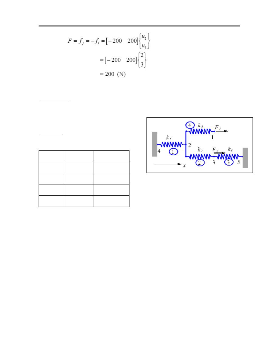
Example-2: For the spring system with arbitrary numbered nodes and elements, as
shown. Find the global stiffness matrix.
Solution:
First construct the following:
Element Node (1)
Node (2)
1
4
2
2
2
3
3
3
5
4
2
1
[ ]
[ ]
[ ]
−
−
=
−
−
=
−
−
=
3
3
3
3
3
5
3
2
2
2
2
2
3
2
1
1
1
1
1
2
4
K
K
K
K
K
u
u
K
K
K
K
K
u
u
K
K
K
K
K
u
u

53
[ ]
[ ]
−
−
−
+
−
−
−
+
+
−
−
=
−
−
=
3
3
1
1
3
3
2
2
1
2
4
2
1
4
4
4
5
4
3
2
1
4
4
4
4
4
1
2
K
0
K
0
0
0
K
0
K
0
K
0
K
K
K
0
0
K
K
K
K
K
K
0
0
0
K
K
K
u
u
u
u
u
K
K
K
K
K
u
u
54
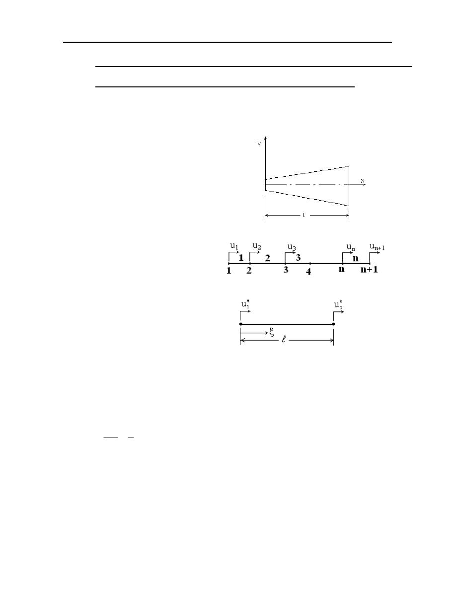
6.4 APPLICATION TO THE UN AXIALLY STRESSED BAR
SUBJECTED TO VARIOUS END CONDITIONS.
1. Defining the finite element mesh.
2. Selecting the displacement model.
We will assume
ξ
+
=
ξ
1
0
e
a
a
u
[ ]
)
1
......(
..........
a
a
1
u
1
0
e
ξ
=
ξ
l
1
0
e
2
0
e
1
a
a
u
a
u
+
=
=
)
2
........(
a
a
1
0
1
u
u
1
0
e
2
e
1
=
l
=
l
1
0
1
A
From equations (1) and (2)
[ ]
−
=
−
l
l
1
1
0
1
A
1
[ ][ ]
ξ
=
∴
−
ξ
e
2
e
1
1
e
u
u
A
1
u

55
e
2
e
1
e
u
u
1
u
l
l
ξ
+
ξ
−
=
ξ
ξ
ξ
−
=
ξ
e
2
e
1
e
u
u
1
u
l
l
( )
[
]
{ }
e
0
u
N
)
(
u
ξ
=
ξ
Where :-
( )
[ ]
=
ξ
N
Shape function.
{ }
=
e
0
u
Displacement vector.
3. Generate the stiffness equilibrium equation.
i- Find the
e
U
: on the basis of equation (1) , the strain
e
ε
"strain within the
element " .
{ }
[ ]
{ }
)
3
(
..........
..........
..........
u
B
u
d
dN
d
du
e
0
e
o
e
=
ξ
=
ξ
=
ε
where
[ ]
−
=
l
l
1
1
B
Hooks law is
σ
=E.
ε
, or in matrix form
[ ] [ ]
}
{
D
ε
=
σ
[ ]
)
4
.........(
..........
dvol
}
{
D
}
{
2
1
dvol
E
2
1
U
t
2
e
ε
ε
=
⋅
ε
⋅
=
∫
∫
Substitute from equation (3) in equation (4) get:
{ }
[ ] [ ] [ ]
{ }
ξ
⋅
Α
⋅
=
∫
d
u
B
D
B
u
2
1
U
e
0
t
0
e
0
e
l
{ } (
[ ] [ ] [ ]
) { }
e
0
0
t
t
e
0
u
d
B
D
B
u
2
1
ξ
Α
⋅
=
∫
l
56
⇒
{ }
[ ]
{ }
e
0
t
e
0
e
u
u
2
1
U
Κ
=
where : [
Κ
]
= element stiffness matrix.
[
Κ
]
=
)
5
....(
..........
..........
..........
..........
1
1
1
1
−
−
ΕΑ
l
ii- To find total energy stored U:
∑
=
e
e
)
6
...(
..........
..........
..........
..........
..........
..........
U
U
it is convenient to express this equation in matrix formation:
{ }
{ }
{ }
{ }
=
−
n
0
3
0
2
0
1
0
u
u
u
u
U
,
[ ]
[ ]
[ ]
[ ]
[ ]
)
7
.........(
k
0
0
0
0
k
0
0
0
0
k
0
0
0
0
k
K
n
3
2
1
=
⇒
{ }
[ ]
{ }
)
8
........(
..........
..........
..........
..........
u
k
u
2
1
U
t
=
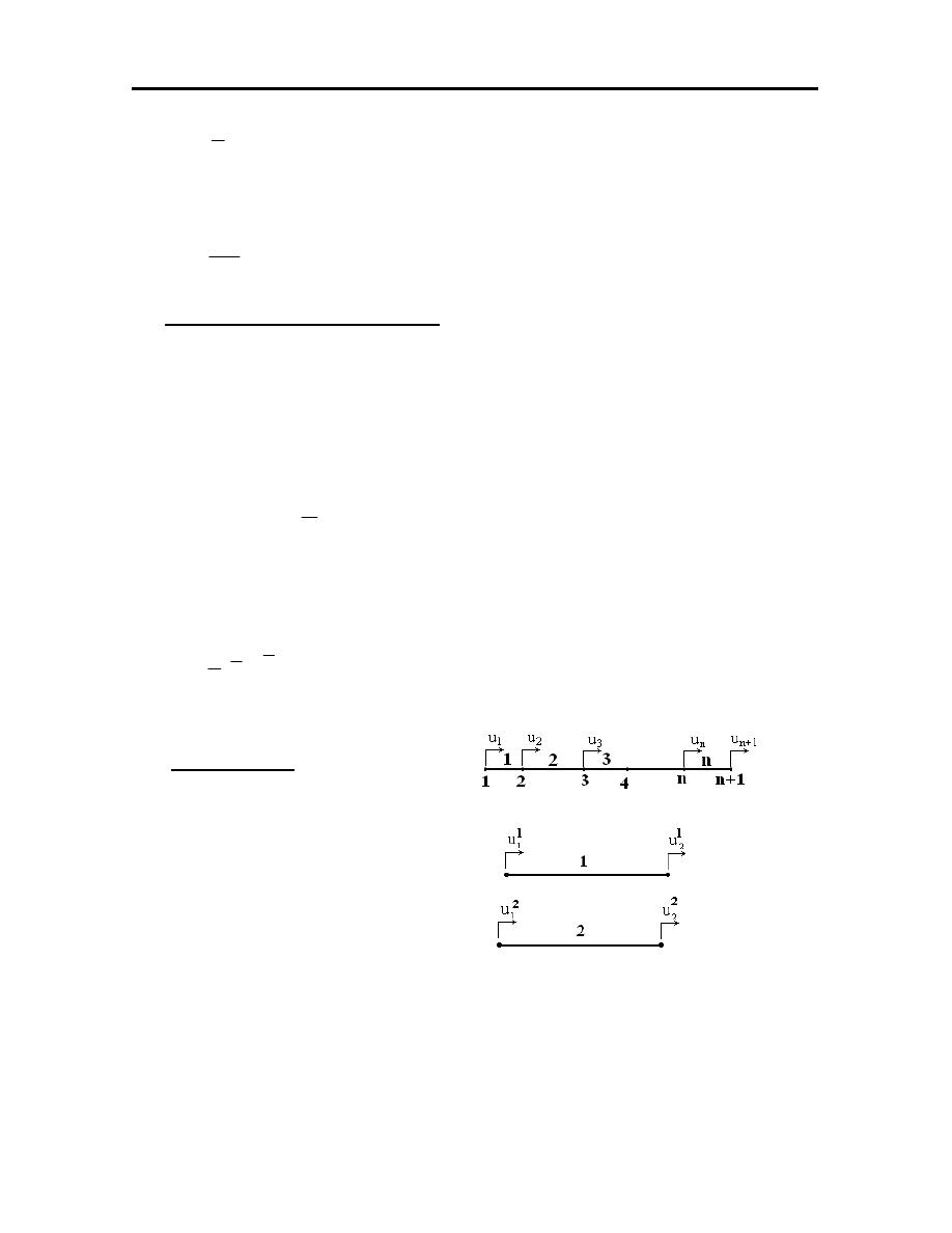
iii- compatibility
for compatibility
1
1
1
u
u
=
2
1
2
u
u
=
2
2
1
u
u
=
3
2
2
u
u
=
and so on

57
⇒
)
9
...(
..........
..........
..........
u
u
u
u
1
0
0
0
0
0
0
0
..........
0
0
1
0
0
..........
0
0
0
1
0
..........
0
0
0
1
0
..........
0
0
0
0
1
u
u
u
u
u
u
n
3
2
1
n
2
n
1
2
2
2
1
1
2
1
1
=
{ }
[ ]
{ }
u
c
u
=
where
[
C
]
= connection compatibility
from equation (9) into (8) get:
=
−
u
c
k
c
u
2
1
U
t
t
{ }
[ ]
{ }
u
k
u
2
1
t
=
where
[Κ]
= system of global or assembly
[ ] [ ]
[ ]
)
10
.......(
..........
..........
..........
..........
..........
c
k
c
k
t
=
−
iv- potential energy of applied loads
As a first case, suppose concentrated axial forces are applied at the nodes (1,2 ,
…., n+1) then:
1
n
1
n
3
3
2
2
1
1
x
u
....
x
u
x
u
x
u
+
+
−
−
−
=
Ω
, where
Χ
is applied load .
or
{ }
[ ]
)
11
.....(
..........
..........
..........
p
u
t
−
=
Ω
v- total potential energy :-
{ }
[ ]
{ } { }
[ ]
p
u
u
k
u
2
1
U
V
t
t
−
=
Ω
+
=
and
58
( { }
[ ]
{ } { }
[ ]
{ }
) { }
[ ]
p
u
u
k
u
u
k
u
2
1
V
t
t
t
δ
−
δ
+
δ
=
δ
since
[Κ]
symmetric
{ } (
[ ]
{ }
[ ]
)
)
12
..(
..........
..........
..........
p
u
k
u
V
t
−
δ
=
δ
But for equilibrium
δν=0 ,
and
{ }
t
u
δ
arbitrary
∴[Κ]{υ}={Ρ}
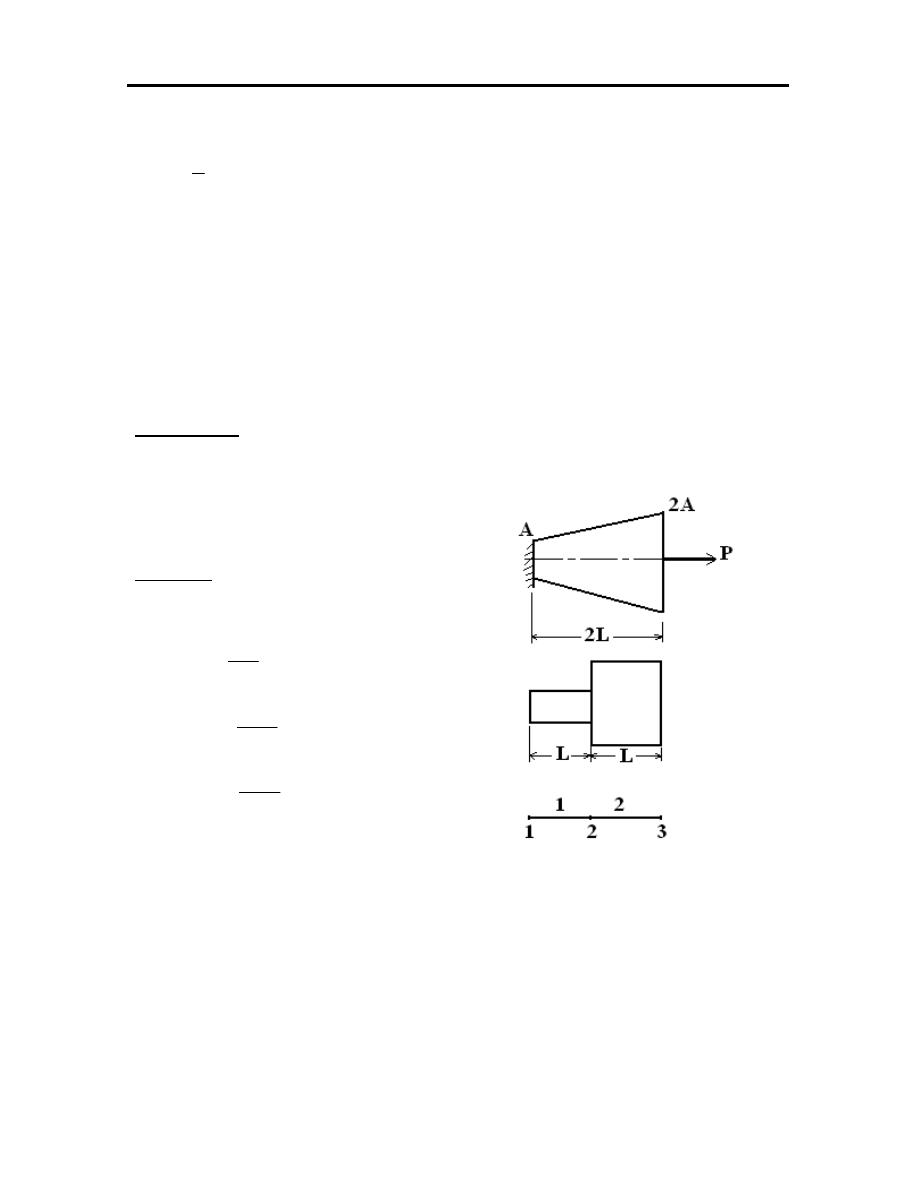
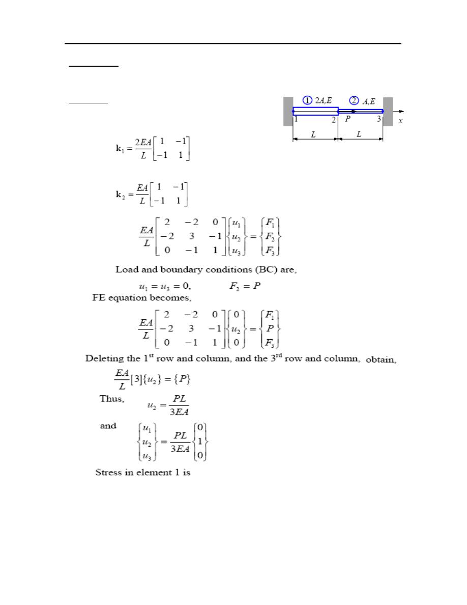
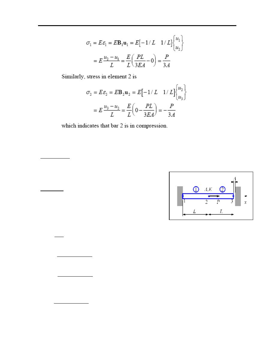
Example-3: Using finite element method to formulate the equilibrium equation
and find the displacement and stresses of the bar subjected to various
end conditions shown.
Solution:
1. Element stiffness matrices:
[ ]
[ ]
[ ]
−
−
=
−
−
=
−
−
=
1
1
1
1
L
4
EA
7
K
1
1
1
1
L
4
EA
5
K
1
1
1
1
EA
K
2
1
l
2. Assembly of [K]
[ ]
+
=
2
22
2
21
2
12
2
11
1
22
1
21
1
12
1
11
k
k
0
k
k
k
k
0
k
k
K

59
[ ]
[ ]
−
−
−
−
=
−
−
+
−
−
=
L
4
EA
7
L
4
EA
7
0
L
4
EA
7
L
4
EA
12
L
4
EA
5
0
L
4
EA
5
L
4
EA
5
K
L
4
EA
7
L
4
EA
7
0
L
4
EA
7
L
4
EA
7
L
4
EA
5
L
4
EA
5
0
L
4
EA
5
L
4
EA
5
K
3. Equilibrium equation:
−
−
−
−
=
=
3
2
1
4
7
4
7
0
4
7
4
12
4
5
0
4
5
4
5
0
}
]{
[
}
{
u
u
u
L
EA
L
EA
L
EA
L
EA
L
EA
L
EA
L
EA
P
R
u
K
P
As the left hand side clamped so (u
1
=0) and therefore:
−
−
=
3
2
u
u
7
7
7
12
L
4
EA
P
0
EA
PL
4
u
7
u
12
49
P
]
u
7
u
7
[
L
4
EA
and
u
12
7
u
0
]
u
7
u
12
[
L
4
EA
3
3
3
2
3
2
3
2
=
+
−
=
+
−
=
⇒
=
−

60
EA
PL
8
.
0
u
EA
PL
371
.
1
u
EA
PL
4
u
12
35
2
3
3
=
=
=
4. Stress in element:
[ ]
{ }
{ }
ε
=
σ
−
=
=
ε
E
and
u
L
1
L
1
u
B
e
0
e
0
For element (1)
[
]
{ }
[
]
[
]
A
P
8
.
0
EA
PL
8
.
0
0
1
1
L
E
u
u
1
1
L
E
u
1
1
L
E
E
2
1
1
0
1
1
=
−
=
−
=
−
=
ε
=
σ
For element (2)
[
]
[
]
A
P
57
.
0
EA
PL
371
.
1
EA
PL
8
.
0
1
1
L
E
u
u
1
1
L
E
E
3
2
2
2
=
−
=
−
=
ε
=
σ
The exact solution
A
P
667
.
0
A
5
.
1
P
center
the
at
A
2
P
A
P
2
1
=
=
σ
=
σ
=
σ
61
Example-4: Find the stresses in the two bar assembly which is loaded with force
P, and constrained at the two ends, as shown in the figure.
Solution:
Use two 1-D bar elements.
62
Example-5: Determined the support reaction forces at the two ends of the bar
shown, if P=60 KN, E=20 GN/m
2
, A=250 mm
2
, L=150 mm, and
Δ=1.2mm.
S0lution:
Δ
o
=PL/EA=(60*10
3
*150)/(20*10
3
*250)=1.8mm
Since Δ
o
=1.8> Δ=1.2, so the contact of the bar
with the wall on the right will occur.
[ ]
[ ]
[ ]
−
−
=
−
−
=
−
−
=
1
1
1
1
150
250
*
10
*
20
K
1
1
1
1
150
250
*
10
*
20
K
1
1
1
1
L
EA
K
3
2
3
1
[ ]
−
−
−
−
=
1
1
0
1
2
1
0
1
1
150
250
*
10
*
20
K
3

63
−
−
−
−
=
3
2
1
3
1
u
u
u
1
1
0
1
2
1
0
1
1
150
250
*
10
*
20
3
F
P
F
Since left side is fixed so u
1
=0 and get:
mm
5
.
1
2
.
1
250
*
10
*
20
10
*
60
*
150
2
1
u
)
u
2
(
150
250
*
10
*
20
P
u
1
1
1
2
150
250
*
10
*
20
F
P
3
3
2
2
3
2
3
3
=
+
=
∆
−
=
∆
−
−
=
To find the support reaction forces:
KN
10
)
2
.
1
5
.
1
(
150
250
*
10
*
20
)
u
u
(
150
250
*
10
*
20
F
KN
50
)
5
.
1
0
(
150
250
*
10
*
20
)
u
u
(
150
250
*
10
*
20
F
3
3
2
3
3
3
2
1
3
1
−
=
+
−
=
+
−
=
−
=
−
=
−
=
64
H.W
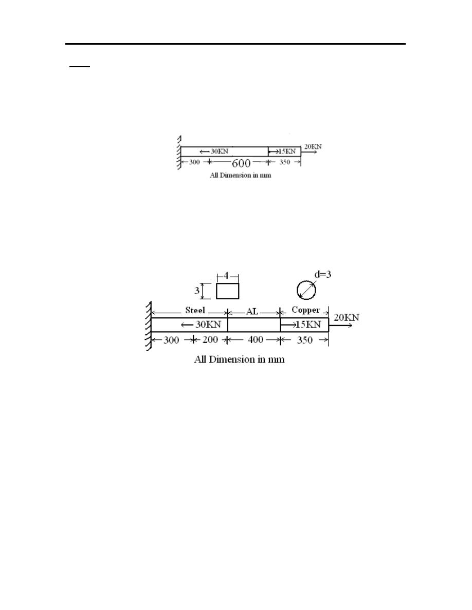
1. Consider a two degree of freedom bar elements as shown in figure. Using finite
element method to formulate the equilibrium equation of it. If the cross
sectional area is 12 mm
2
and E=200 GN/m
2
.
2. Consider a two degree of freedom bar element as shown in figure. Using finite
element method to formulate the equilibrium equation of it, and then estimate
the stress distributions. If E
steel
=200 GN/m
2
, E
Copper
= 110GN/m
2
and E
AL
= 120
GN/m
2
.
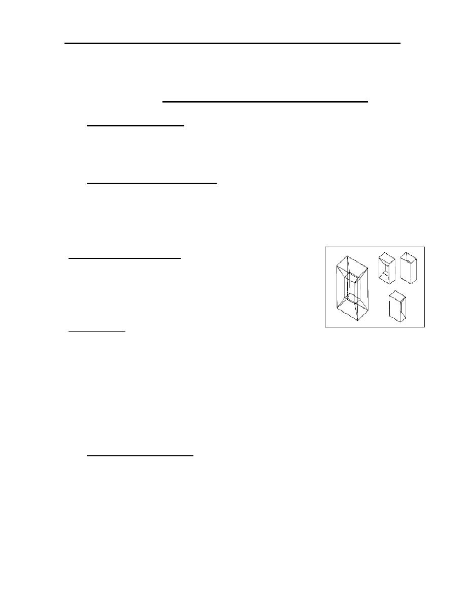
65
CHAPTER FIVE
GEOMETRIC MODELING
5.1 INTRODUCTION
Geometric models in CAD/CAM can be based on a wire frame, surface
models or solid models.
5.2 WIRE FRAME MODEL
The wire frame model is represented by tables defining edges and points
of the shapes. The coordinates (x,y,z) of each point are stored in the points-table.
This model can not be used to determine surface area or volume of an object.
Mathematic description:
– A list of curve equations;
– Coordinates of points; and
– Connectivity information for shape curves and points.
Advantages:
1. Require simple user input;
2. Easy for users to develop systems by themselves.
• Disadvantages:
1. Ambiguous in shape;
2. No information about inside and outside boundary surface.
5.3 SURFACE MODEL
The surface model is represented by tables of edges and points as a wire
frame plus a table of faces. A record of faces stores edges from which the face is
consist.
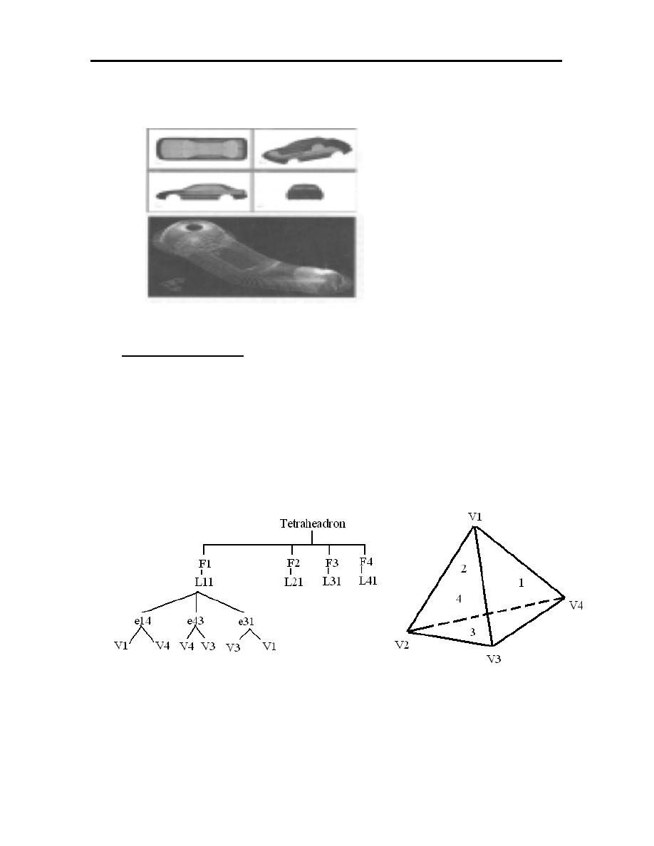
66
This model can be used to determine surface area only but can not used to
determine volume or moment of inertia.
5.4 SOLID MODEL
The solid model is represented in either of the following ways:
1. Boundary representation of solid model: it has information on the faces,
edges and vertices plus topological information which defines the
relationships between the faces, edges and vertices. So the solid is
represented as closed space in 3-D space.
2. Constructive solid geometry: using Boolean operations, the solid object is
made from two intersecting solid primitives. The operations consist of
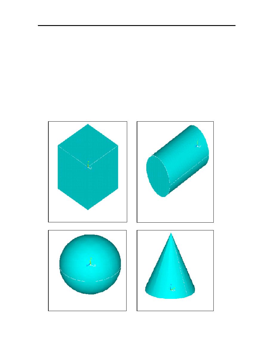
67
union, intersection and difference or subtraction. The basic 3-D primitives
are:
a- Block (box)
b- Cylinder
c- Sphere
d- Cone
e- Torus
f- Wedge
c- Sphere
d- Cone
a- block
b- cylinder
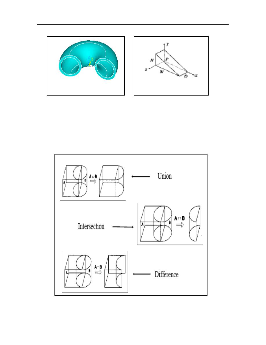
68
In which the Boolean operations are:
a. Union: combines two volumes into a single solid.
b. Intersect: keeps only the volume common to both solid objects.
c. Subtract: the volume of one solid object from the other solid.
e- torus
f- wedge
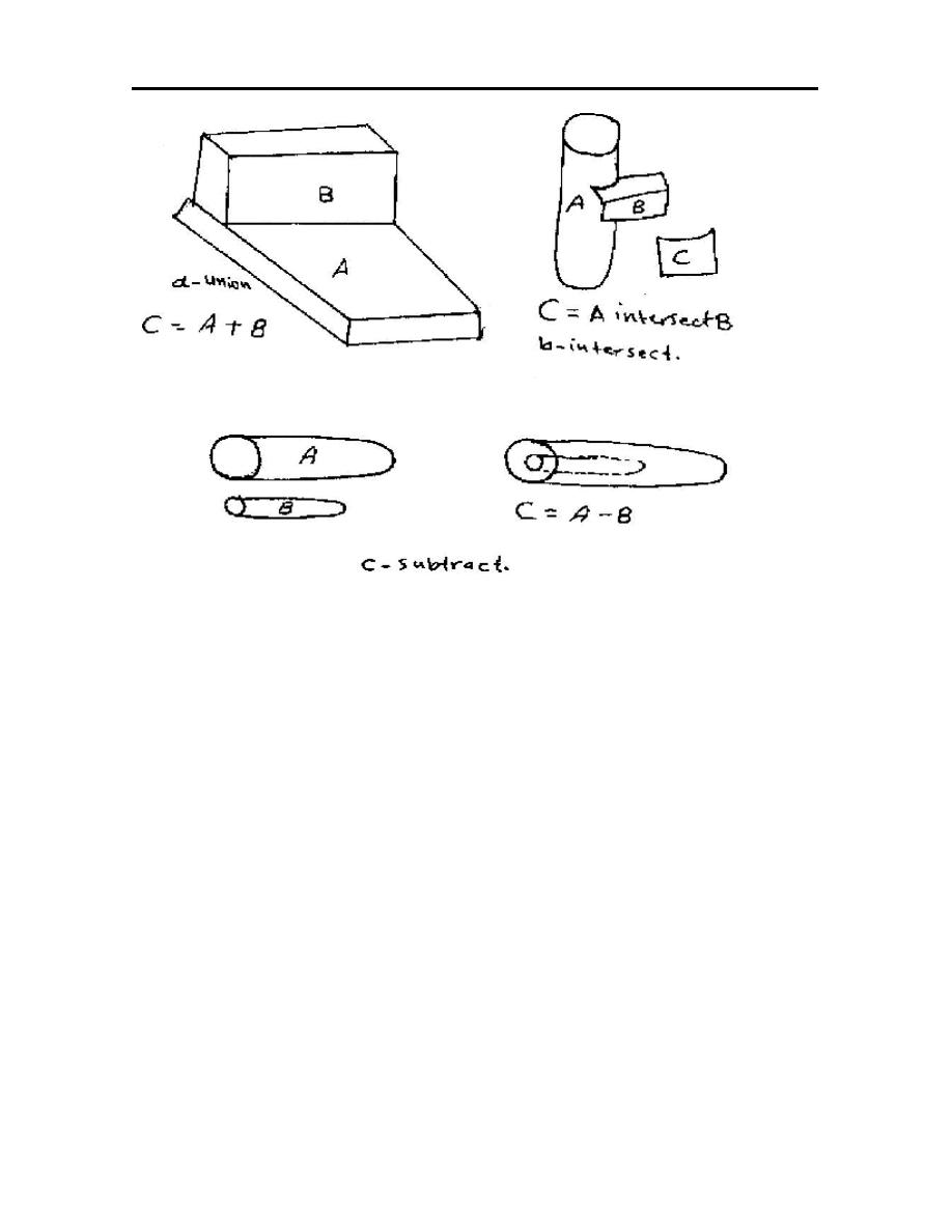
69
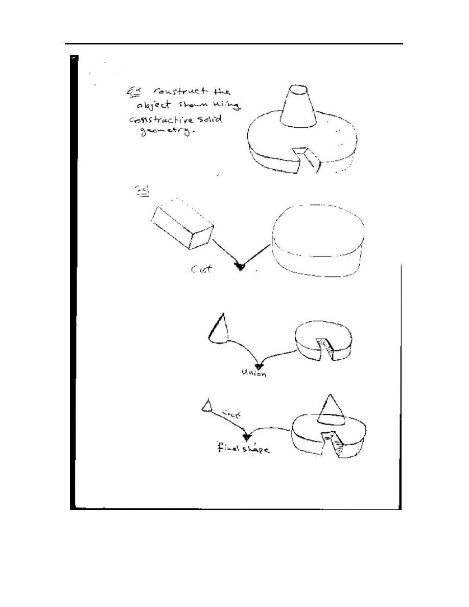
70
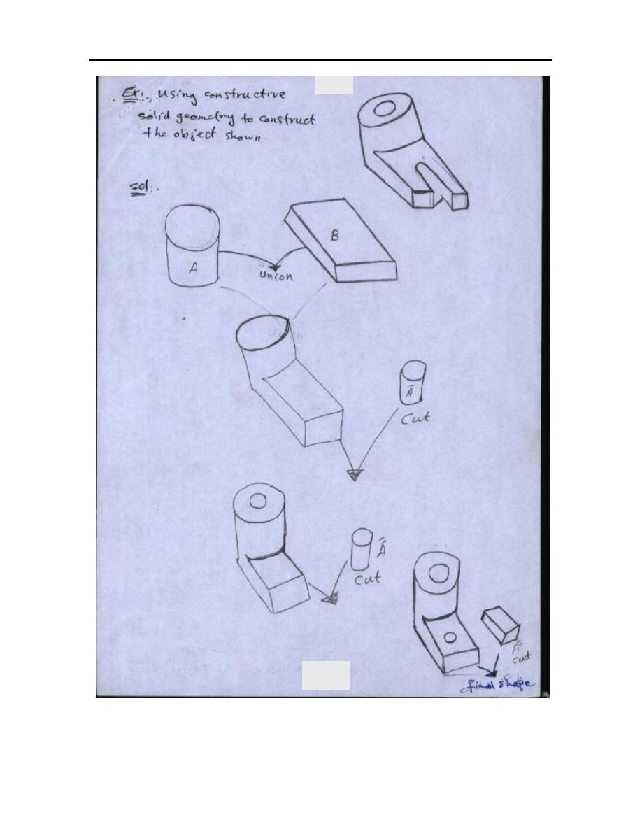
71
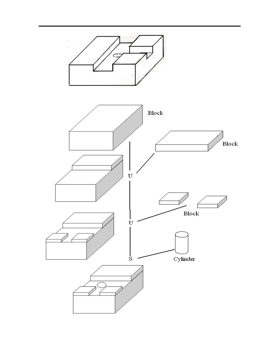
72

73
CHAPTER SIX
SYSTEM DESIGN AND MANUFACTURE
6.1 MANUFACTURING PRODUCTION CYCLE
The manufacturing production cycle consist of many steps that:
1. Processing operation:
a. Basic process (metal casting, plastic molding).
b. Secondary process (milling, turning, drilling…).
c. Process to enhance physical properties (heat treatment, surface
treatment).
d. Finishing operation (polishing, painting).
2. Assembly operation:
a. Mechanical fastening (screw, rivet, nut…….).
b. Joining process (welding, soldering ……).
3. Material handling and storage:
a. Transporting between successive operations.
b. Transporting to final stage.
4. Control:
a. Inter stage control.
b. Final stage control.
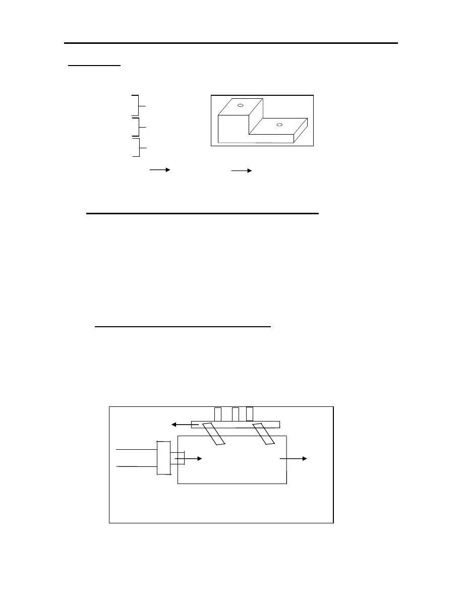
74
Example-1: List the main operations required to produce the shape shown.
1. Cutting
2. Milling
3. Drilling
4. Grinding
5. Final control final storage assembly.
6.2 METHOD OF WORKPIECE TRANSPORT
1. Continuous transfer mechanism:
•
Easy to design.
•
High rate of production.
2. Intermitted transfer mechanism:
•
Greater flexibility.
6.2.1 TYPE OF TRANSFER MECHANISM
There are two types of transfer mechanism that linear and rotary
mechanism:
1. Linear transfer mechanism:
a. Walking beam.
Piston
Table
Input-Linear movement.
Output- Linear movement.
. .
. .
I.C
I.C
I.C
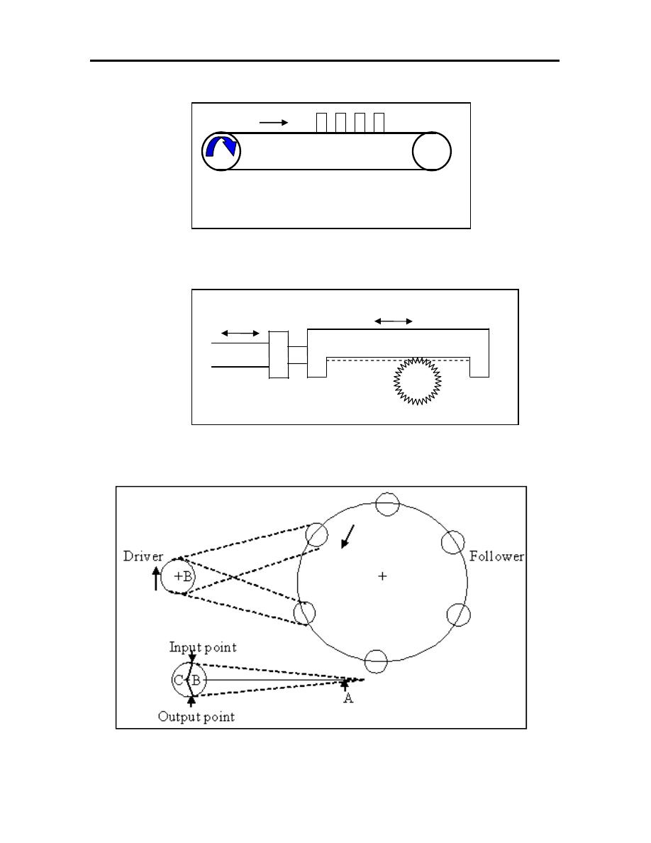
75
b. Conveyor.
2. Rotary transfer mechanism:
a. Rack and pinion.
b. Geneva mechanism:
Indexing table
Rack
Piston
.
Pinion
.
+
Input-Rotary.
Output-Linear.

76
time
Cycle
1
Rate
oduction
Pr
360
B
Angle
C
Angle
180
B
A
180
90
B
2
1
A
2
1
time
Dwell
time
Index
time
Cycle
=
=
+
=
+
=
+
+
+
=
o
o
o
Example-2: An index table driven by a Geneva mechanism has six stations with a
driver speed of 12rpm calculate: Index time, Dwell time, Cycle time
and production rate.
Solution:
.
hr
/
721
3600
9
.
4
1
time
Cycle
1
rate
oduction
Pr
sec
99
.
4
33
.
3
66
.
1
time
Dwell
time
Index
time
Cycle
.
sec
33
.
3
min
0555
.
0
12
1
360
240
time
Dwell
C
time
Dwell
.
sec
66
.
1
min
0277
.
0
12
1
360
120
time
Index
B
time
Index
240
120
360
C
360
B
C
120
60
180
B
180
B
A
60
6
360
A
Angle
=
=
=
=
+
=
+
=
=
=
×
=
α
=
=
×
=
α
=
−
=
=
+
=
−
=
=
+
=
=
o
o
o
o
o

77
6.3 AN AUTOMATION BLOCK BUILDING
The basic component of automation as primarily belonging to one of the
following:
1. Sensors: sensors are first link between the typical automation system and
conventional process. The most sensors type are:
•
Manual switches.
•
Proximity switches: Some switch do not require physical contact or
light radiation to sense an object. Such switch is called proximity
switches.
•
Photo electric sensors: In wider use than proximity switches are
sensors that are sensitive to light radiation. Two approaches for
employing photoelectric are in use:
a. The first approach merely uses a photocell to detect the presence of light
radiating naturally from some object in the process.
b. The second approach to photoelectric employs a beam of light emitted by
an artificial light source. The principal purpose of this approach is to
detect the presence or absence of objects in the path of the beam
•
Infrared Sensors: Sometimes it is useful to detect electromagnetic
radiation outside the visible range. Infrared sensors respond to
radiation in the range of wave length just beyond the visible spectrum
at the red end. Infrared sensors are very useful when used with
artificial beams to detect the presence or absence of objects, even
more than Photo electric systems.
•
Fiber optical: Convenient supplement to Photo electric or infrared
sensor systems are fiber optic light tubes, which are flexible pipes of
glass or plastic that can be used to bend light beams around corners.
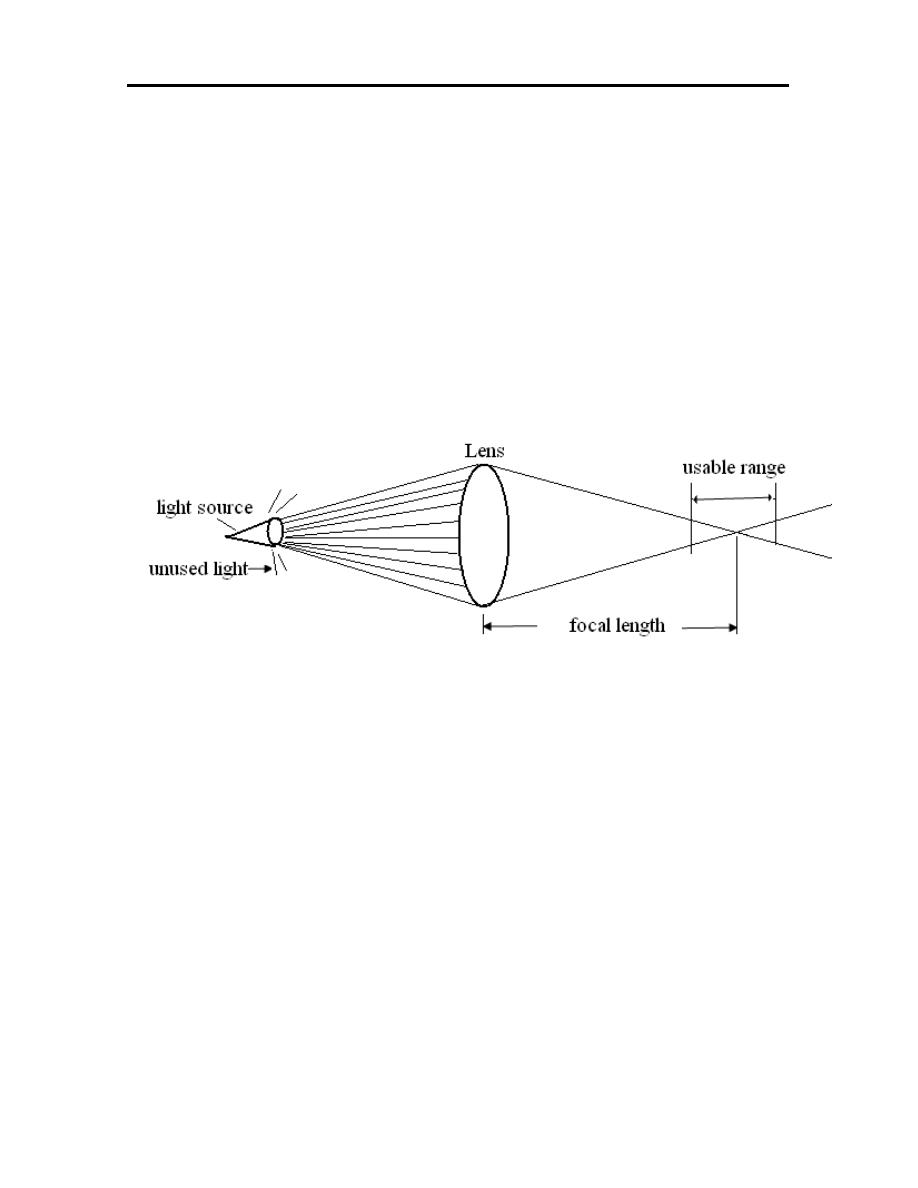
78
Fiber optics are so efficient that it becomes worthwhile for the
telephone industry to convert communications circuits from
electrical signals to modulated light signals for transmission via
fiber optics and subsequent reconversion at the receiving end.
•
Laser: In automated systems, the laser is useful in providing very
long, precise light beams. The precision of the beams makes them
excellent for detecting tiny objects that are capable of breaking the
beam at large and varying distances. Such precision also makes the
laser a good tool for dimensional measurement.

79
2. Analyzer: information is sensed by automated system it must be registed and
analyzed and then decision must be made by the system as to what action
should be taken. The analyzers type are:
•
Computers: Digital computers are primary means of analyzing
automation system inputs. Computers are extremely versatile in that
the ways they can be programmed to manipulate data are limitless.
•
Counters: It is frequently useful for an automated system to
determine how many of various items are present or pass through an
automated system. The counter can be mechanical, solid state
electronic counters.
•
Timer: If pieces clock pulses are available, a counter that counts
these pulses becomes a timer basically a clock. An industrial timer is
more similar to an alarm clock than an ordinary clock. When the
elapsed time becomes equal to a preset value, an output signal is
generated.
•
Bar Code Readers: is an analyzing system that incorporates a
conventional photoelectric or laser scanner along with timers and
counters.
•
Optical Encoder: The capability of rapidly scanning. It’s a series of
bars make possible additional automation opportunities when light and
dark bars are placed concentric rings on a disk. A portion of such a
disk that can be rigidly attached to a shaft and housed in an assembly
consisting of optical sensors for each ring. The assembly is called an
optical encoder and is useful for automatically detecting shaft rotation.

80
Beam of light passes through slots in a disk and are detected by a light
sensor. When the disk is rotated, a pulsed output is produced by the
sensor, with the number of pulses being proportional to the angle
through which the disc rotates. Angular rotation of disc (shaft rotation)
can be determined by the number of pulses produced since some
reference position.
A= Angular value of ring (i).
m
i
= 0 If the ring is white.
m
i
= 1 If the ring is dark.
n= Total number of rings.
Example-3: An absolute optical encoder disk has eight rings and eight LED
sensors and turn to provide eight bit output. Suppose the output
pattern is [10010110], what is the angular position of the shaft?
Solution:
Encoder ring inner
Angular value
Observed pattern
Computed value
1
180
1
180
2
90
0
0
3
45
0
0
4
22.5
1
22.5
5
11.25
0
0
6
5.625
1
5.625
7
2.8125
1
2.8125
8
1.40625
0
0
210.9375ْ
∑
=
=
n
1
i
i
i
A
m
A

81
3. Actuators: The real world condition is sensed of analyzed some thing may
need to be done about it (Automated system are closing the loop by taking
physical action automatically without operator intervention). Some of the
actuators used are:
•
Cylinder actuators: are defined by their ability to exert a linear force and
hold it at any specified position indefinitely. The cylinder actuators
divided into hydraulic and pneumatic actuators.
•
Solenoids.
•
Relay.
4. Drivers: It takes some action upon the process at the command of computer
or other analyzed and this action is taken by continuous movement typified by
rotation. There are many type of drivers used such as:
•
Motors.
•
DC servomotors.
•
Stepper motors.
•
Kinematic linkage.
•
Walking beams.
•
Geneva.
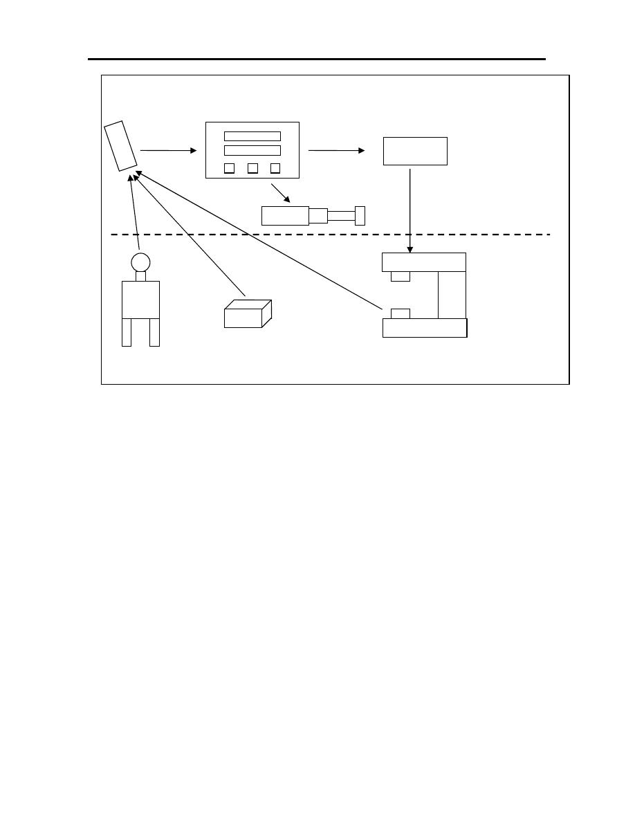
82
Sensors Analyzer
Driver
Automation
components
Actuators
General
manufacturing
process
Operator Piece Process machine

83
CHAPTER SEVEN
FUNDAMENTAL OF NUMERICAL CONTROL
7.1 INTRODUCTION
The (NC) machine is one type of the programmable machine, controlled the
machine tool by a special program for each work piece required. The program
consists of (numbers, letters and etc) precise instructions about the methodology
of manufacture as well as the movement, for example, what tool to be used, at
what speed, at what feed to move from which point to which point in what path,
and then saved on the punched tape. The punched tape read by the control device.
When replaced the work piece required to product the program must be replaced
also, these style made the (NC) machine suitable for low and mid production.
7.2 BASIC COMPONENT OF (NC) SYSTEM
The general structure of the operation of a typical numerical control system
is shown in figure below. The (NC) machine must be consisting of the following
components:
1. Program of instruction.
2. Control unit.
3. Machine tool.
The part program consist of instructions written in the numerical codes
constitute the basic operations to be carried out in machining of the part. These
instructions are then entered into an input medium such as a paper tap. The
program is then read by paper tape reader. The controller translates these
numerical codes into the machine actuation details, which are then used to control
the individual machine functions such as the movement of the axes.
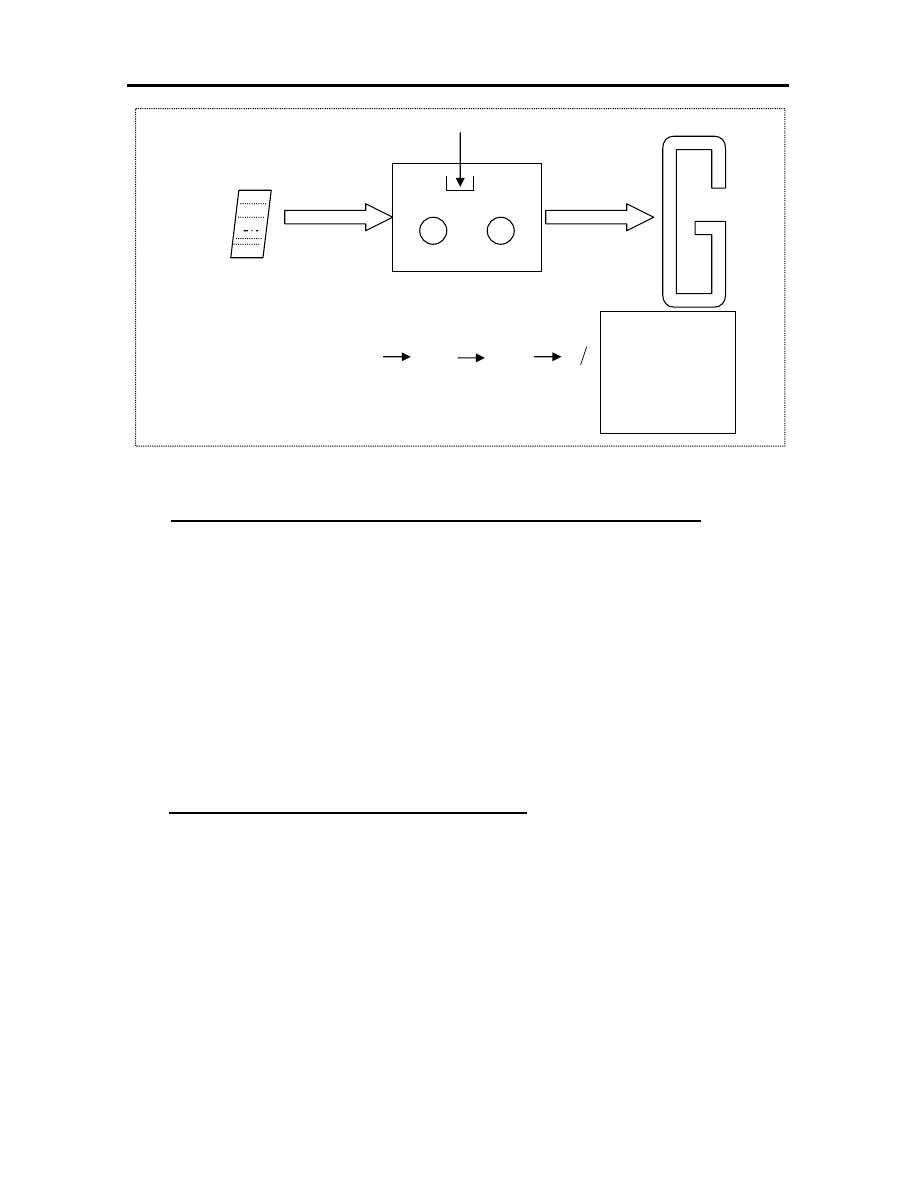
84
7.3 CLASSIFICATION OF NUMERICAL CONTROL
Numerical control (NC) machines can be classified as follows:
1. Control loops.
2. Motion control.
3. Power drives.
4. Hardwired (NC) and softwired computer numerical control (CNC).
5. Positioning systems.
1. CONTROL LOOPS OF (NC) SYSTEM
The control loops of (NC) system are designed to control the position and
velocity of the machine tool axis. There are two types of control systems in the
programmable machines; open loop and closed loop. The overall accuracy of the
machines is determined by the type of control loop used.
The open loop control system doesn’t positioning feedback to the control
unit. The movement pulses are sent out by the control unit and they are received
Input
-punched tape
-data carrier
Sensor
Control unit
-punch tape reader
Read data buffer signal
C
M
-Table
-Spindle
-Motors
-Control
-Data display
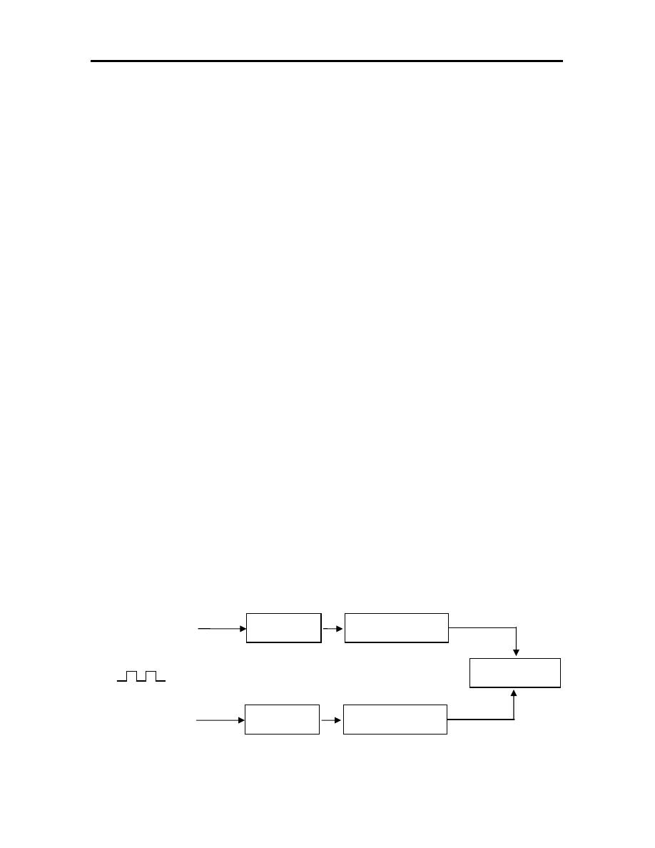
85
by a special type of servomotor called a stepper motor. The number of pulses that
the control sends to the stepper motor controls the amount of the rotation of the
motor. The stepper motor then proceeds with the next movement command. Since
this control system only counts pulses and can’t identify discrepancies in
positioning, the control has no way of knowing that the tool not reaches the proper
location. The machine will continue this inaccuracy until somebody finds the
error. The advantage of the open loop control system is that it is less expensive,
since it doesn’t require the additional hardware and electronics needed for
positioning feedback. The disadvantage is difficulty of detecting a positioning
error.
In the closed loop control system the electronic movement pulses are sent
from the control to the servomotor, enabling the motor to rotate with each pulse.
The movement are detected and counted by a feedback deviance called
transducer.
With each step of movement, a transducer sends a signal back to the
control, which compares the current position of the driven axis with the
programmed position. When the number of pulses sent and received match, the
control starts sending out pulses for the next movement.
Drive unit
Stepping motor
Machine table
Drive unit
Stepping motor
y-axis
y-axis
x-axis
x-axis
Command pulses
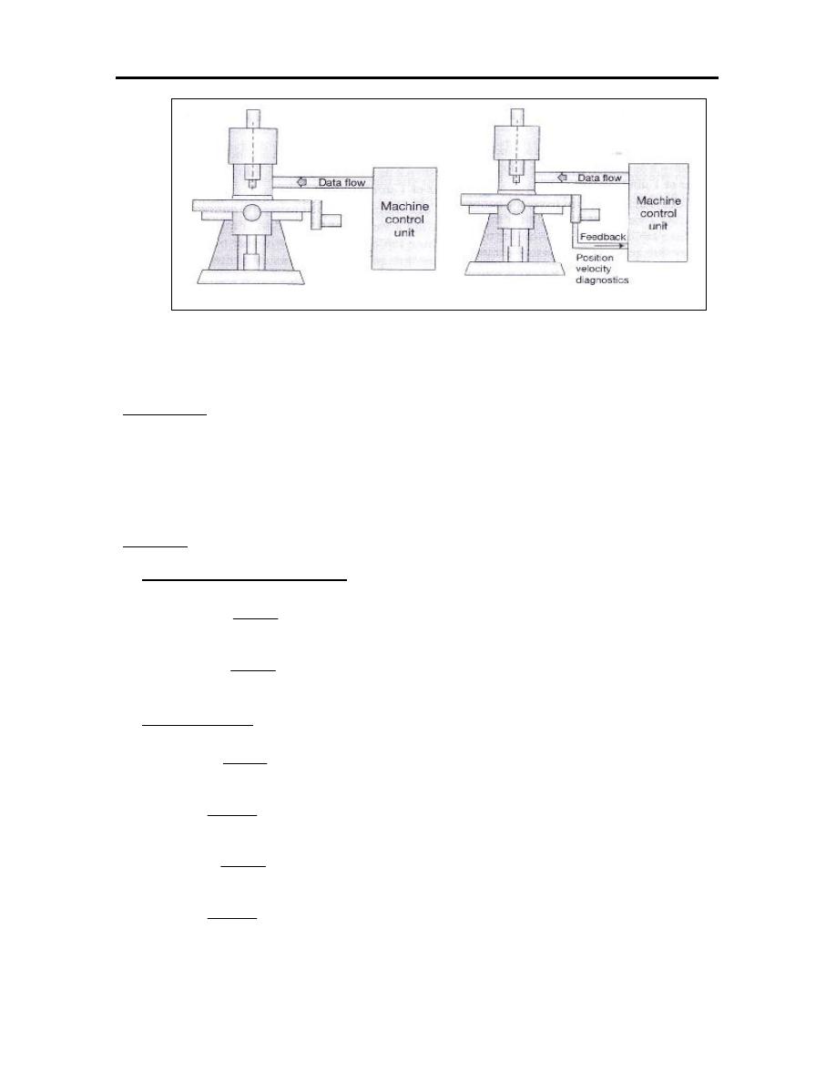
86
Example-1: Calculate the displacement in accuracy of (NC) system without
velocity feed back for the following motion:
N09 G01 X82.55 Y44.45 F100
Take the smallest programmable increment is (0.002) mm/pulses.
Solution:
►Number of required pulses:
pulses
22225
002
.
0
45
.
44
Y
pulses
41275
002
.
0
55
.
82
X
pulses
pulses
=
=
=
=
►Time intervals:
.
sec
/
pulses
33
.
833
67
.
26
22225
.
sec
67
.
26
min
4445
.
0
100
45
.
44
Y
.
sec
/
pulses
33
.
833
53
.
49
41275
.
sec
53
.
49
min
8255
.
0
100
55
.
82
X
time
time
=
⇒
=
=
=
=
⇒
=
=
=
Open loop NC machine Closed loop NC machine

87
►X-error:
mm
033
.
0
5129
.
82
55
.
82
mm
5129
.
82
002
.
0
41258
pulses
41258
833
53
.
49
=
−
=
×
=
×
►Y-error:
mm
0178
.
0
4322
.
44
45
.
44
mm
4322
.
44
002
.
0
11
.
2216
pulses
11
.
2216
833
67
.
26
=
−
=
×
=
×
2. MOTION CONTROL OF (NC) SYSTEM
There are three types used to control the motion in (NC) system:
1. Point to point positioning control.
2. Straight-cut positioning control.
3. Continuous (contouring) path (NC) system.
The function of PTP motion control system is to move the machine table or
spindle to a specified position to perform the machining operation at that point.
The path taken to reach the specific point is not defined by the programmer in this
system. Because this movement is nonmachining, as shown in figure below there
are some paths that may be taken between the two point P and Q. a PTP-NC
machine is able to perform simple milling operations if the machine is equipped
with feed control mechanism. With most PTP machines, the only directions that
are accurately controlled are straight lines parallel to the machine axes (right and
left, forward and backward).
In continuous control system, the machine control two or more axes
simultaneously. The tool contacts the workpiece and the desired shapes are made
as shown.
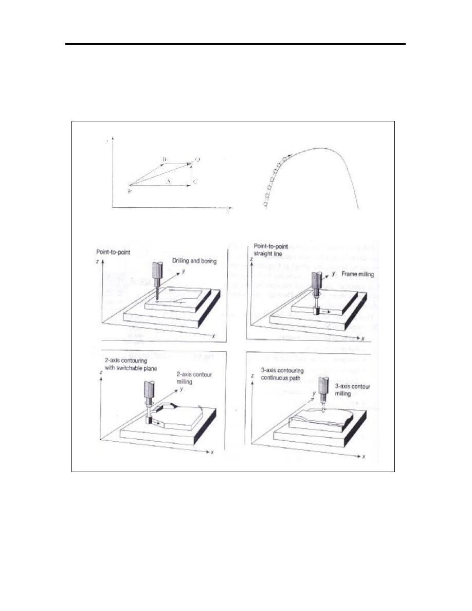
88
PTP motion control Continuous path control
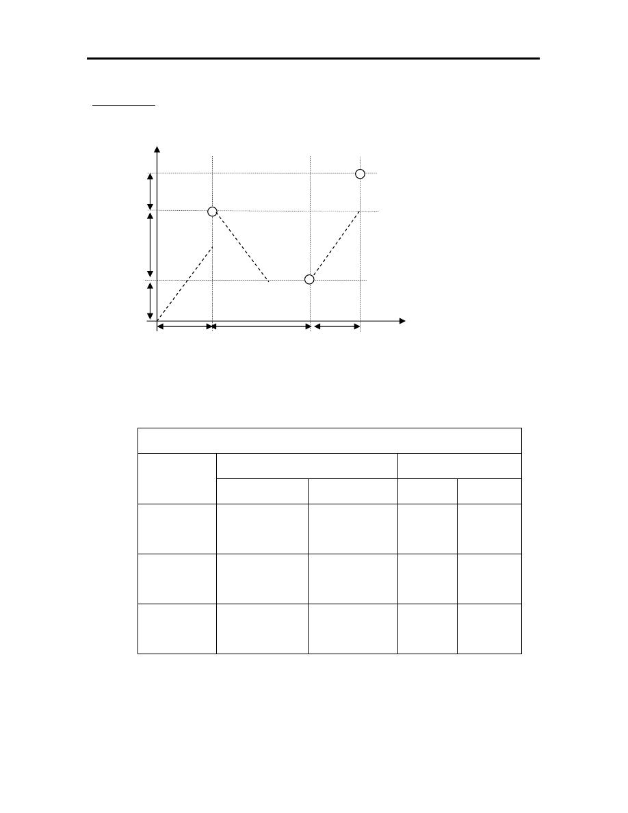
89
Example-2: Define the path of three holes in figure below.
The tool path may be Sequential (parallel to the axes) or Simultaneous (by 45˚)
thus:
Path of 3-holes
Tool path
motion
Sequential
Simultaneous
From
To
X25Y35
0-a-1
0-c-1
0-b-1
0
1
X50Y-20
1-d-2
1-f-2
1-e-2
1
2
X20Y30
2-h-3
2-g-3
2-i-3
2
3
Y
g 3
10
C 1 f i
20 b
d e 2 h
15
a
0 25 50 20 X
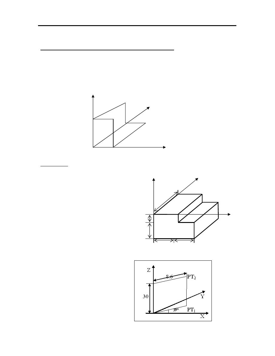
90
Mathematics for programming coordinate system
1. Cartesian coordinate system:
Point PT[x,y,z]
Line L[PT
1
,PT
2
]
Plane PL[PT
1
,PT
2
,PT
3
]
Example-3: using Cartesian coordinate to locate the point in the figure shown.
2. Polar coordinate system:
Point [radius, angle]
PT
1
[R,A]
PT
1
[8.6,39˚]
PT
2
[R,A,Z]
PT
2
[8.6,39˚,30]
0 1
-10
4
-20
6
20 20
Z Y
2
35
3 5
X
PT
0
=[0,0,0]
PT
1
=[20,0,0]
PT
2
=[20,35,0]
PT
3
=[20,35,-10]
PT
4
=[20,0,-10]
PT
5
=[40,35,-10]
PT
6
=[40,0,-30]
Z-axis
Y-Z
Y-axis
Plane
X-Z
Plane X-Y
Plane
X-axis
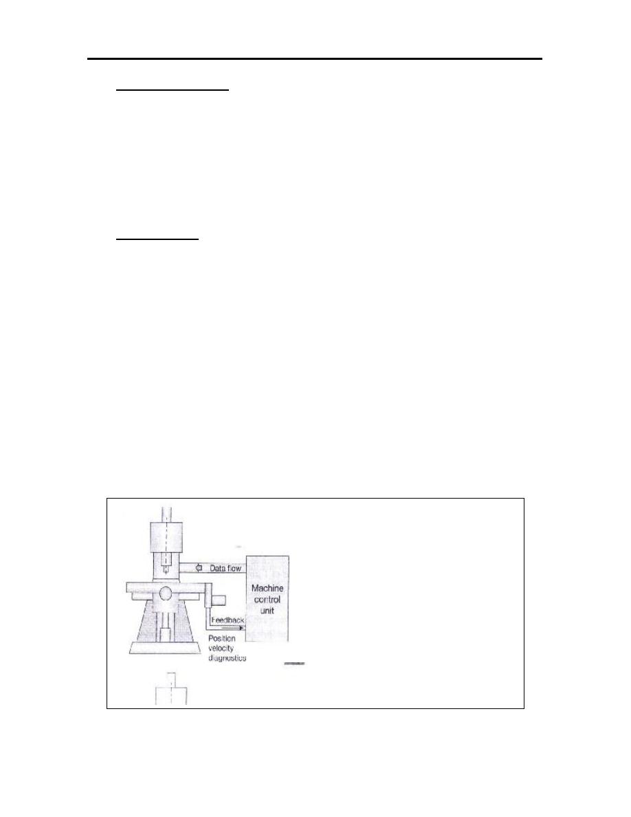
91
3. POWER DRIVES
Most modern NC machines are use DC or AC servo motor to drive the
axes and the spindle. Their small size, ease of control, and low cost are
advantages of servo motor. In large machines hydraulic drives are used. Also
pneumatic drives are rarely used in NC positioning system.
4. NC and CNC
The difference between NC and CNC lies in the controller technology.
The NC machines developed in the early days had the total control system
developed using the hardware. This is sometimes called hardwired numerical
control. These are characterised by a part program input media such as
magnetic or paper tape. These had very little part program memory.
The new control systems are termed as computer numerical control
(CNC) which are characterised by the availability of computer and enhanced of
memory in the controller as shown in the figure.

92
CNC machines have many advantages over conventional machines.
Some of them are:
1. There is a possibility of performing multiple operations on the same
machine in one setup.
2. Because of the possibility of simultaneous multi-axis tool movement,
special profile tools are not necessary to cut unusual part shapes.
3. The scrap is significantly reduced because of the precision of the CNC
machine and lesser operator impact.
4. It is easy to incorporate part design changes when CAD/CAM systems
are used.
5. It is easy to perform quality assurance by spot-check instead of
checking all parts.
6. Production is significantly increased.
CNC machines also have some disadvantages:
1. They are quite expensive.
2. They have to be programmed, set up, operated, and maintained highly
skilled personnel.
5. POSITIONING SYSTEMS
In general there are two methods to define the tool location:
1. Absolute: Tool location always defined in relation to zero point.
2. Increment: The next tool position must be defined with reference to the
previous tool location.
Note: In increment of the polar coordinate the angle only vary.
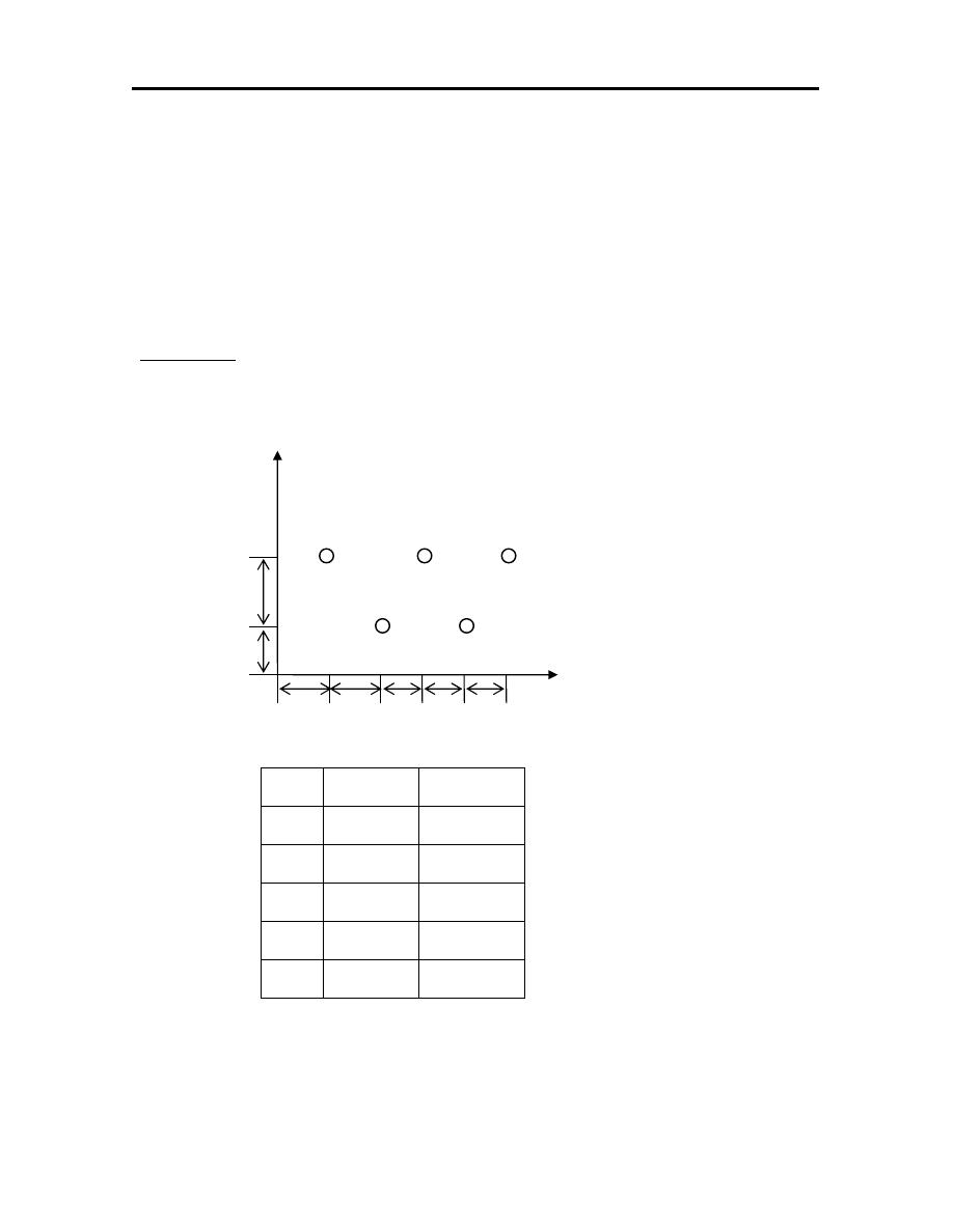
93
Modern NC machines also allow the user to choose the types of
positioning systems through software. In an absolute positioning system NC
machine, the coordinate origin also can be reset. Machines that allow their
coordinate origin to be reset are called floating zero machines; other called
fixed zero machines.
Example-4: Locate the position of the points shown using absolute and
increment.
Y
1 3 5
14
2
4
8
10 10 10 10 10 X
Point Absolute Increment
1
(10,22)
(10,22)
2
(20,8)
(10,-14)
3
(30,22)
(10,14)
4
(40,8)
(10,-14)
5
(50,22)
(10,14)
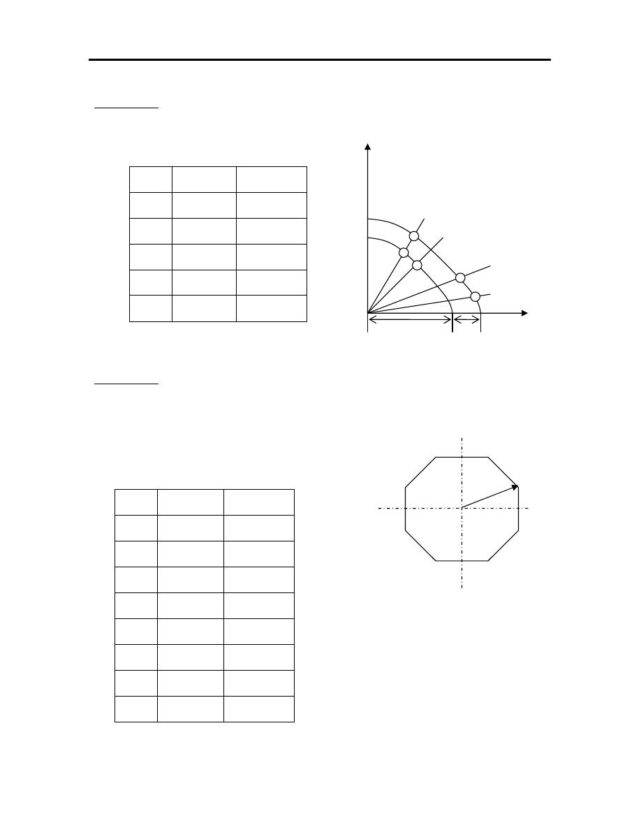
94
Example-5: Using absolute and increment methods to locate the position of the
points shown.
Example-6: Using absolute and increment methods to locate the tool position of
the octagonal object with radius of 30.
2
1
3
8
30
4 7
5 6
Point Absolute Increment
1
(30,45˚)
(30,45˚)
2
(30,90˚)
(30,45˚)
3
(30,135˚)
(30,45˚)
4
(30,18˚)
(30,45˚)
5
(30,225˚)
(30,45˚)
6
(30,270˚)
(30,45˚)
7
(30,315˚)
(30,45˚)
8
(30,360˚)
(30,45˚)
Angle=360/8=45˚
Y
75˚
5
60˚
4
3 30˚
2
1
10˚
40 20 X
Point Absolute Increment
1
(60,10˚)
(60,10˚)
2
(60,30˚)
(60,20˚)
3
(40,60˚)
(40,30˚)
4
(40,75˚)
(40,15˚)
5
(60,75˚)
(60, 0˚)

95
CHAPTER EIGHT
CNC MACHINES PART PROGRAMMING
8.1 INTRODUCTION
Since its introduction, CNC technology has found many applications,
including lathes and turning centers, milling machines and machining
centers, punches, electrical discharge machines, flame cutters, grinders, and
testing and inspection equipment. The most complex CNC machine tools are
the turning center and the machining center.
When preparing a program for a particular operation the programmer
must select all cutting data using recommendations for conventional
machining. This includes proper selection of cutting speeds, feed rates, tools
and tool geometry, and so on. When the programmer has chosen all of the
necessary information property, the operator loads the program into the
machine and presses a button to start the cutting cycle. The CNC machines
moves automatically from one machining operation to another, changing the
cutting tool and applying the coolant. In a surprisingly short time the work
piece is machined according to the highest quality standards.
8.2 AUTOMATIC TOOL CHANGER
Most of the time, several different cutting tools are used to produce
a part. The tools must be replaced quickly for the next machining operation.
For this reason, the majority of CNC machine tools are equipped with

96
automatic tool changer ATC. For the automatic tool changer to operate, it is
necessary to have the following:
1. A tool magazine.
2. The tool adaptor that has a provision for pick-up the tool change arm.
3. The ability in the control to perform the tool change function.
4. Tool change procedure.
The tool magazines to be used have to be considered in terms of the
following attributes:
•
Storage capacity.
•
Type and shape.
•
Tool change procedure.
Storage capacity typically starts with about 12 and can go as high as 200
while 30 to 60 appears to be the most common capacity of the tool
magazines. The simplest type of tool magazine is turret. This method
combines tool storage with the tool change procedure, without need for the
tool change arm. The turret simply indexes to bring the tool into the position
of machining, since the spindle is combined with the tool turret. It is a
simple method and the time is normally more for actual tool change.
The next type of tool magazine found in most of the machine tools with
lower tooling requirements is the drum or disc type magazine. The drum
rotates for the purpose of tool change to bring the required tool to the tool
change arm. For storing large number of tools, a chain type tool magazine
provides the necessary flexibility. The chain allows for a very large variety
of arrangements.
The tool change time range from as low as 2 to a maximum of 10
seconds.
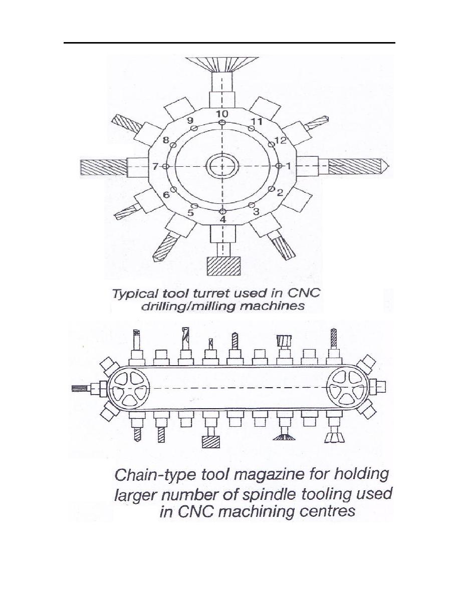
97
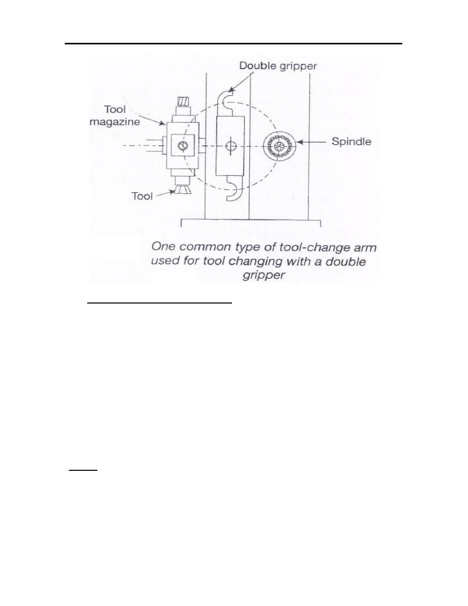
98
8.3 COORDINATE SYSTEMS
In NC system, each axis of motion is equipped with a separately controlled
driving source. The relative movement between tools and workpiece is
achieved by the motion of the machine tool slides. The three main axes of
motion are referred to as the X, Y, and Z.
The Z-axis is perpendicular to both the X and Y axes in order to create
a right hand coordinate system. A positive motion in the Z direction moves
the cutting tool away from the workpiece.
Z-axis
1. On a workpiece-rotating machine, such as a lathe, the Z axis is
parallel to the spindle, and the positive motion moves the tool away
from the workpiece.

99
2. On a tool-rotating machine, such as a drilling or milling machine, the
Z axis is parallel to the tool axis, and the positive motion moves the
tool away from the workpiece.
3. On other machines, such as a press, a planning machine, or shearing
machine, the Z axis is perpendicular to the tool set, and the positive
motion increases the distance between the tool and the workpiece.
X-Axis
1. On a lathe, the X axis is the direction of tool movement, and the
positive motion moves the tool away from the workpiece.
2. On a horizontal milling machine, the X axis is parallel to the table.
3. On a vertical rnilling machine, the positive X axis points to the right
when the programmer is facing the machine.
The Y axis is the axis left in a standard Cartesian coordinate system.
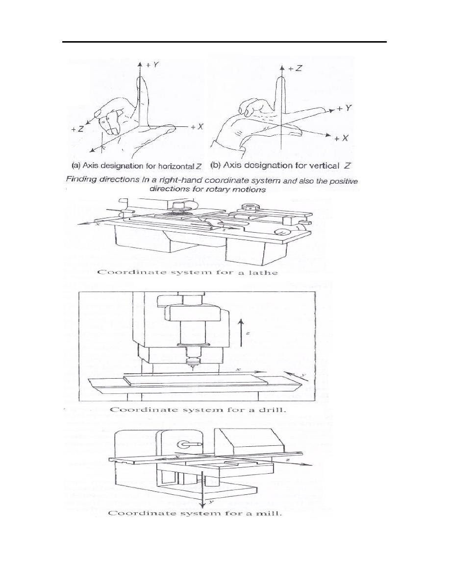
100
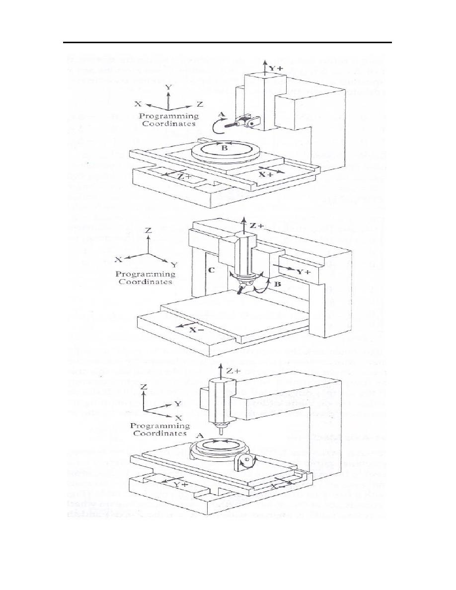
101
102
8.4 AN INTRODUCTION TO PART PROGRAMMING
There are two types of formatting language that the (APT) and
(G-function). The G-function is the main one, while the APT consider is the
secondary language. The G-function codes are classified into:
1. G Codes (Preparatory functions).
2. M Codes (Miscellaneous functions).
To write any program three steps must be apply that:
1. Partitioning the drawing into main parts.
2. List the coordinates of the points.
3. Write the program steps.
Any line programming consist of some functions and written as:
N10 G01 X14 Z26 F3 S150 T12 M8 EOB
Block
number
Function
Dimensional deformation
Feed rate
Spindle speed
Tool number
Miscellaneous function
End of block
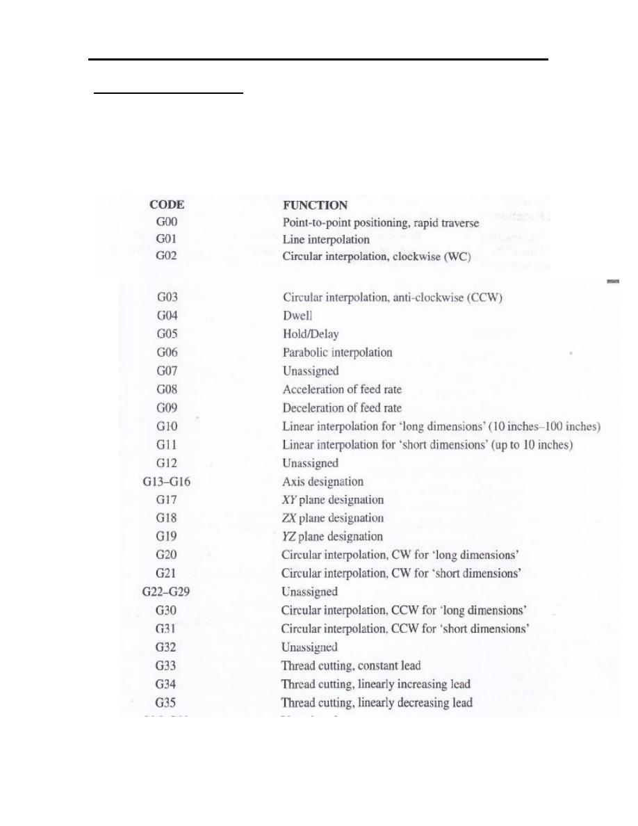
103
Prepartory functions
This is genoted by “G”. it is pre-set function associated with the movement
of machine axes and the associated geometry. It has two digits e.g., G01,
G42, and G90 as per ISO pspecifications. However, some of the current-day
controllers accept up to 3 or 4 digits. Here, we will only discuss some of the
regular functions. ISO has standardised a number of these preparatory
functions, also popularly called G code. The standardised code are:
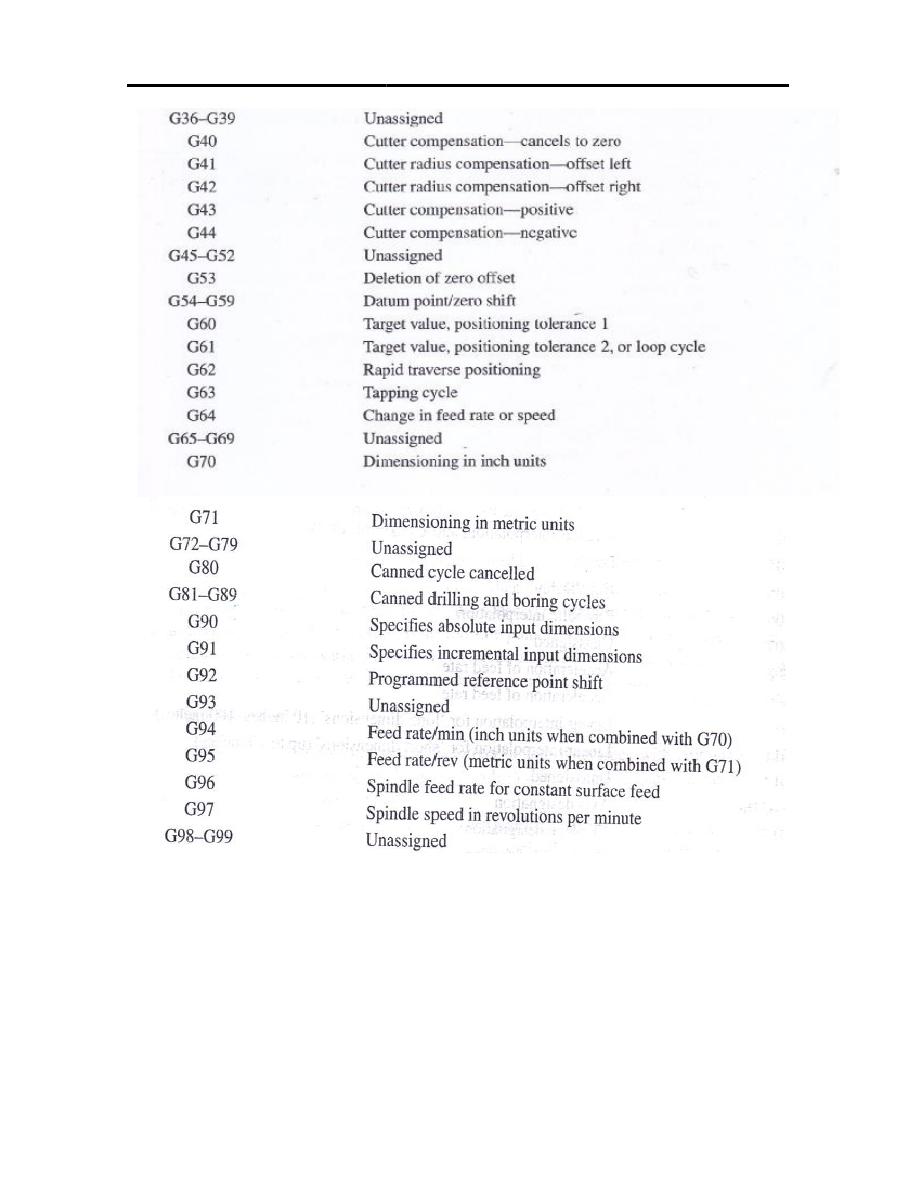
104
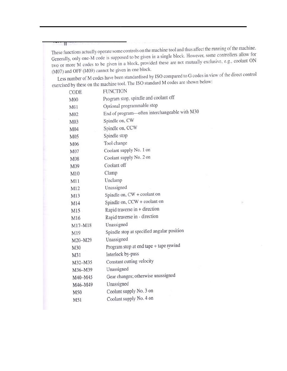
Miscellaneous function, M
105
Miscellaneous function, M
106
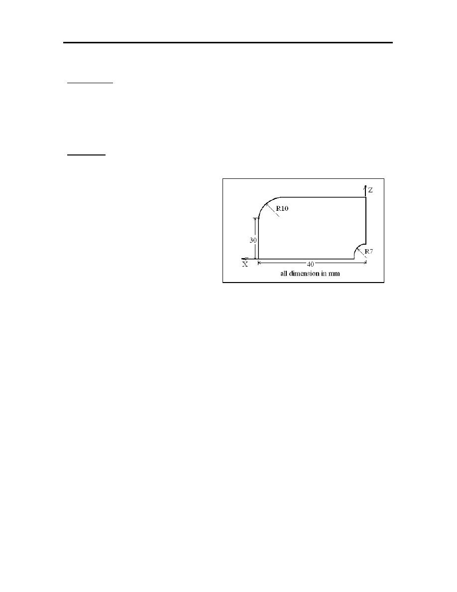
107
Example-1: Using G-function to write the appropriate program for machining
the shape shown, using 10mm/min feed and 500 rpm and tool
number (1).
Solution:
%
01003
N1 G71
N2 G18 M3
N3 M8 G90 S500 F10 T1
N5 G0 X0 Z0
N6 G1 X40 Z0
N7 G1 X40 Z30
N8 G2 X30 Z40 I-10 J0
N9 G1 X0 Z40
N10 G1 X0 Z7
N11 G3 X7 Z0 I0 J-7
N12 M5
N13 M9
N14 M30
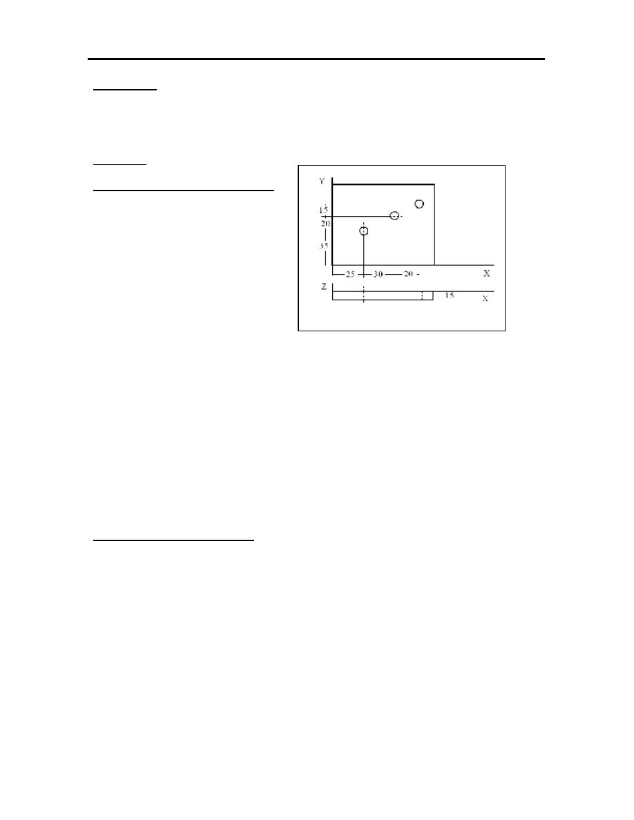
108
Example-2: The component shown to be machined. Write a program without
and with using canned cycles to drill all the holes.
Solution:
Without using canned cycles:
%
01301
N1 G71
N3 G00 X25 Y35 Z2
N4 G01 Z-18 F125
N5 G00 Z2
N6 X55 Y55
N7 G01 Z-18 F125
N8 G00 Z2
N9 X75 Y70
N10 G01 Z-18 F125
N11 G00 Z2
N12 X0 Y0 Z30
With using canned cycles:
%
01302
N1 G71 G17
N2 G81 X25 Y35 Z-18 R2 F125
N3 X55 Y55
N4 X75 Y70
N5 G80 X0 Y0 Z30
All dimension in mm
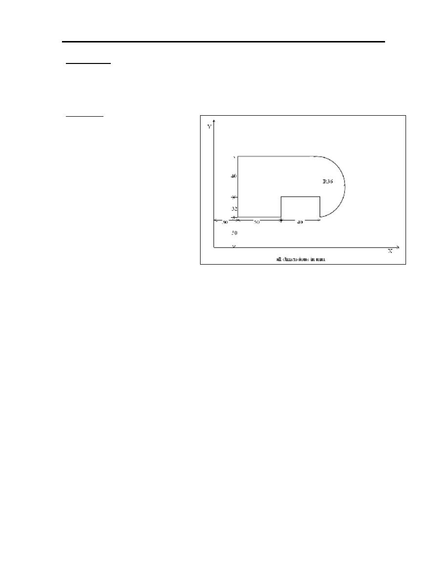
109
Example-3: Write the G-code steps required to obtain the motion statement for
machining the part shown in figure. Using absolute coordinate
system, F20 mm/min and S400 rpm.
Solution:
%
01003
N01 G71
N02 G17
N03 G90 F20 S400
N04 G0 X30 Y50
N05 G1 X80 Y50
N06 G1 X80 Y82
N07 G1 X120 Y82
N08 G1 X120 Y50
N09 G3 X120 Y122 I0 J36
N10 G1 X30 Y122
N11 G1 X30 Y50
N12 G0 X0 Y0
N13 M30
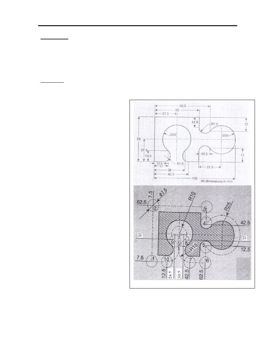
110
Example-4: A complete part program using the ISO codes for the external
contour of the following component shown in the figure. If the stock
dimension is (105*60*5) mm, end mill size is15 mm, feed
100mm/min and 800 rpm speed.
Solution:
%
01313
N10 G71 G92 X0 Y0 Z50
N15 G90 T01 S800 M06
N20 G00 X-7.5 Y-7.5 Z2
N25 G01 Z-6 F100
N30 X-7.5 Y62.5
N35 X62.5 62.5
N40 X62.5 Y42.5
N45 G02 X62.5 Y12.5 R-25
N50 G01 X62.5 Y-7.5
N55 X42.5 Y-7.5
N60 G02 X30.5 Y21 R15
N65 G03 X24.5 Y21 R-10
N70 Go2 X12.5 Y-7.5 R15
N75 G01 X-7.5 Y-7.5
N80 G00 Z2
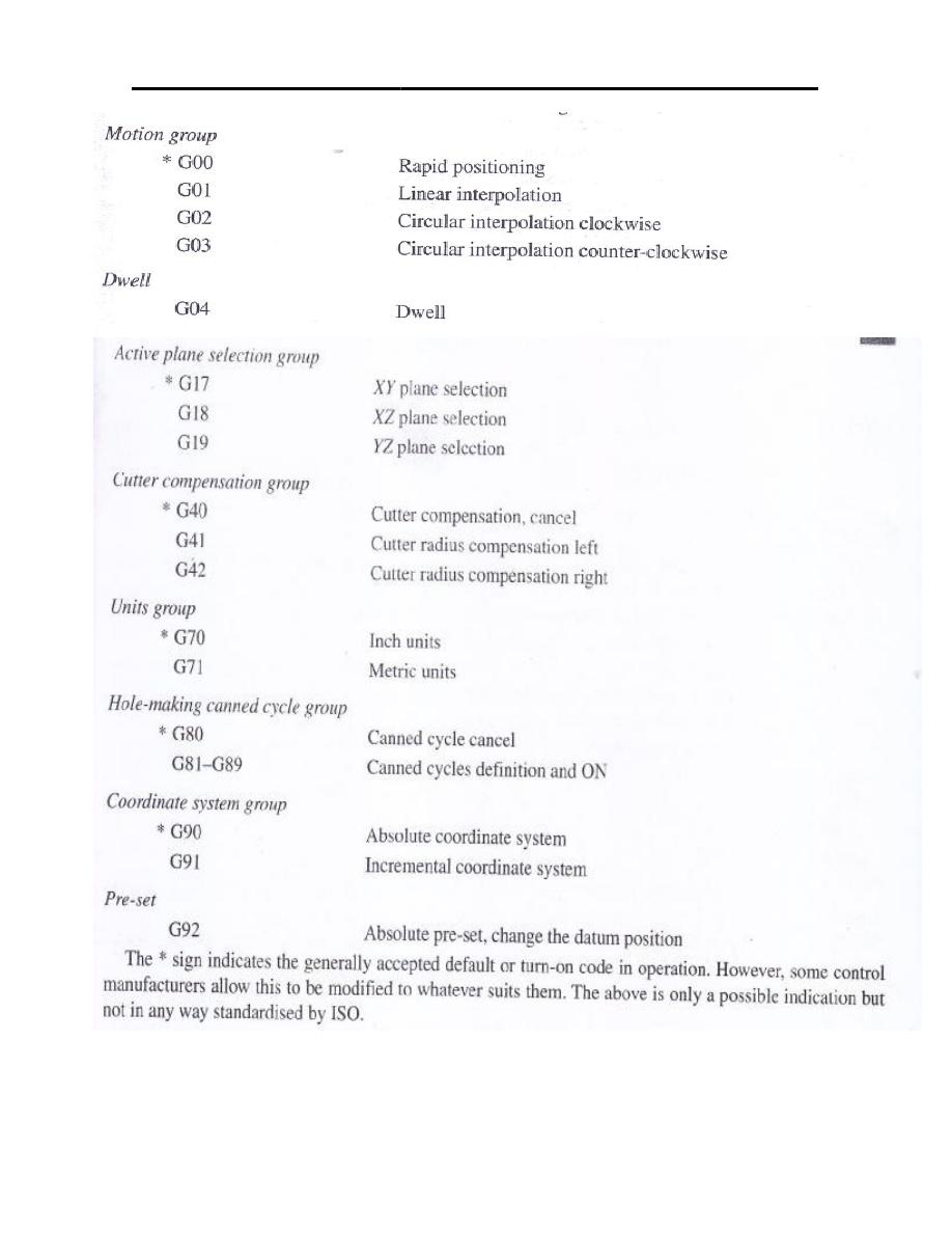
111
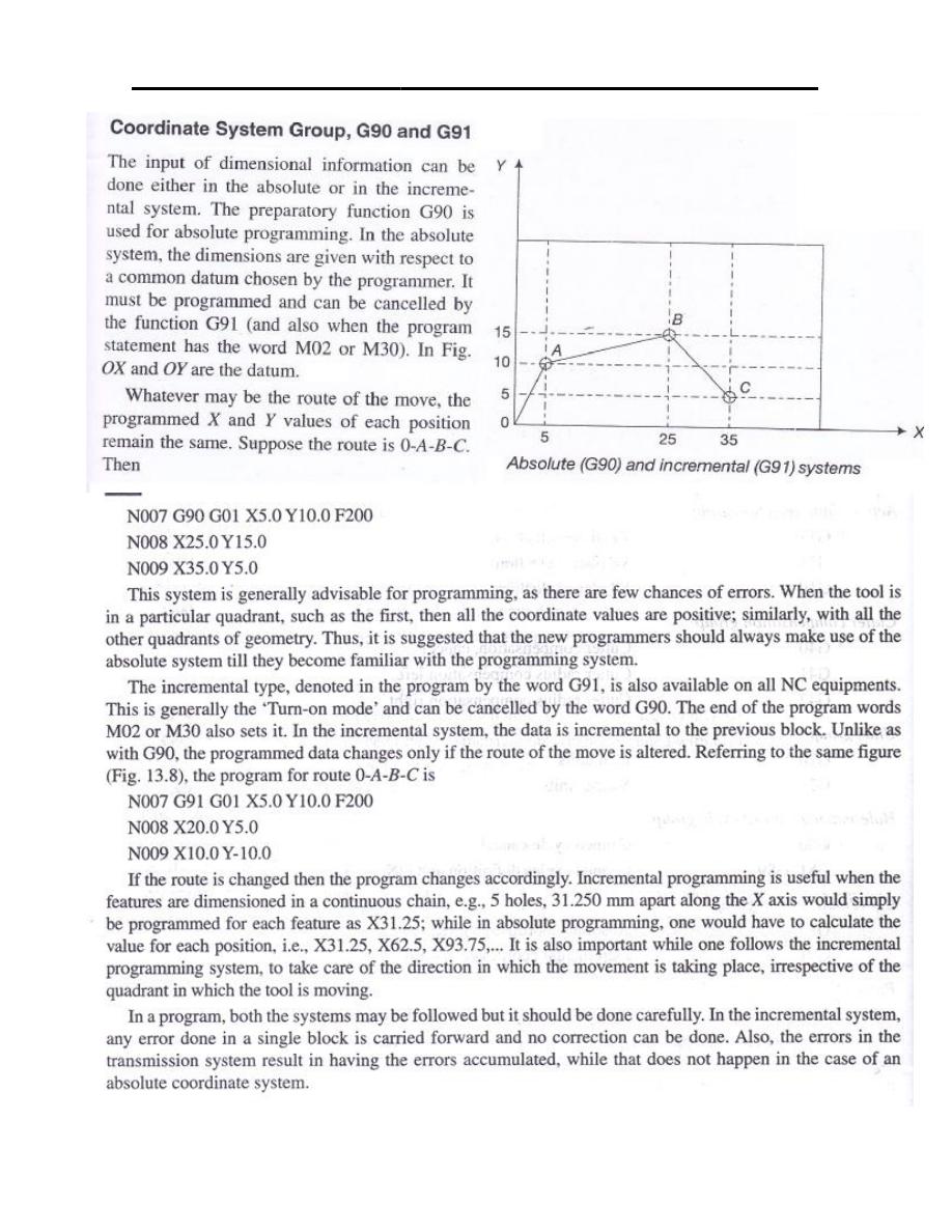
112
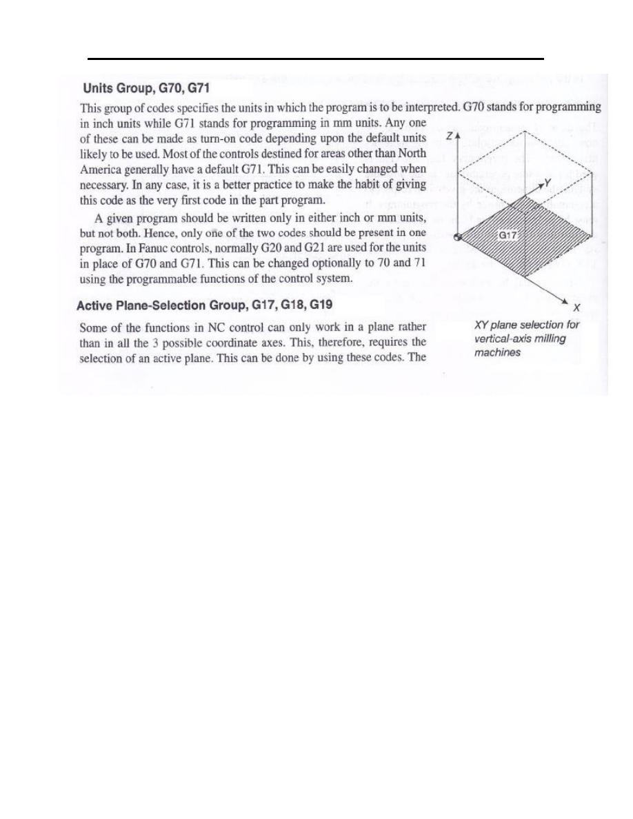
113
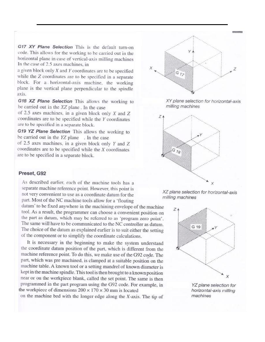
114
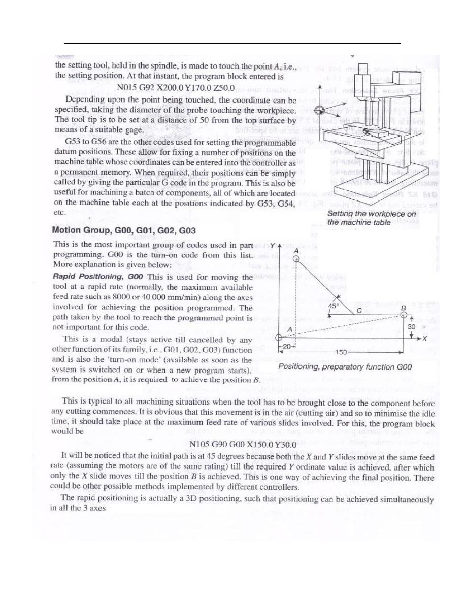
115
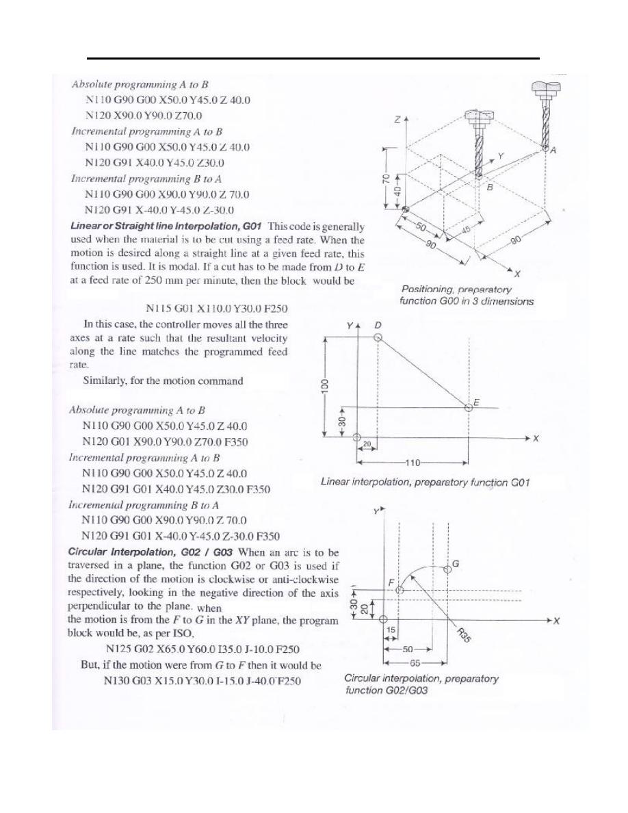
116
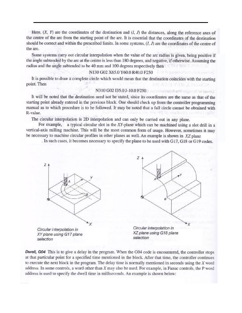
117