
1
PROPERTIES AND STRENGTH OF MATERIALS
Dr. Muhannad Zedan
References
(1) Mechanics of Materials By: E. J. HEARN
(
2) Strength of Materials By: K. William
(3) Alloys: Preparation, Properties, Applications By: Fathi Habashi
(4) Materials for Engineers and Technicians By: Raymond A. Higgins
(5) Engineering Materials Science By: Milton Ohring
PDF created with pdfFactory Pro trial version
2
SIMPLE STRESS AND STRAIN
1. Load (P) (N)
In any engineering structure or mechanism the individual components will be
subjected to external forces arising from the service conditions or environment in which
the component works.
0
,
0
P
,
0
P
Y
X
=
Σ
=
Σ
=
Σ
o
M
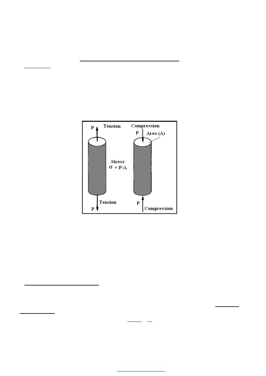
If a cylindrical bar is subjected to a direct pull or push along its axis as shown in
Figure (1), then it is said to be subjected to tension or compression.
Figure (1) Types of direct stress (Tension or Compression)
In the SI system of units load is measured in newtons, loads appear in SI multiples, i.e.
kilonewtons (kN) or meganewtons (MN). There are a number of different ways in which
load can be applied to a member. Typical loading types are:
(a) Static or dead loads, i.e. non-fluctuating loads, generally caused by gravity effects.
(b) Liue loads, as produced by, for example, lorries crossing a bridge.
(c) Impact or shock loads caused by sudden blows.
(d) Fatigue, fluctuating or alternating loads.
2. Direct or normal stress (
σ
),(N/m
2
)
A bar is subjected to a uniform tension or compression, i.e. a direct force, which is
uniformly or equally applied across the cross section, then the internal forces set up are
also distributed uniformly and the bar is said to be subjected to a uniform direct or
normal stress, the stress being defined as
A
P
area
Load
Stress
=
=
PDF created with pdfFactory Pro trial version
3
Stress
(σ)
may thus be (i) compressive stress or (ii) tensile stress depending on the
nature of the load and will be measured in units of (N/m
2
).
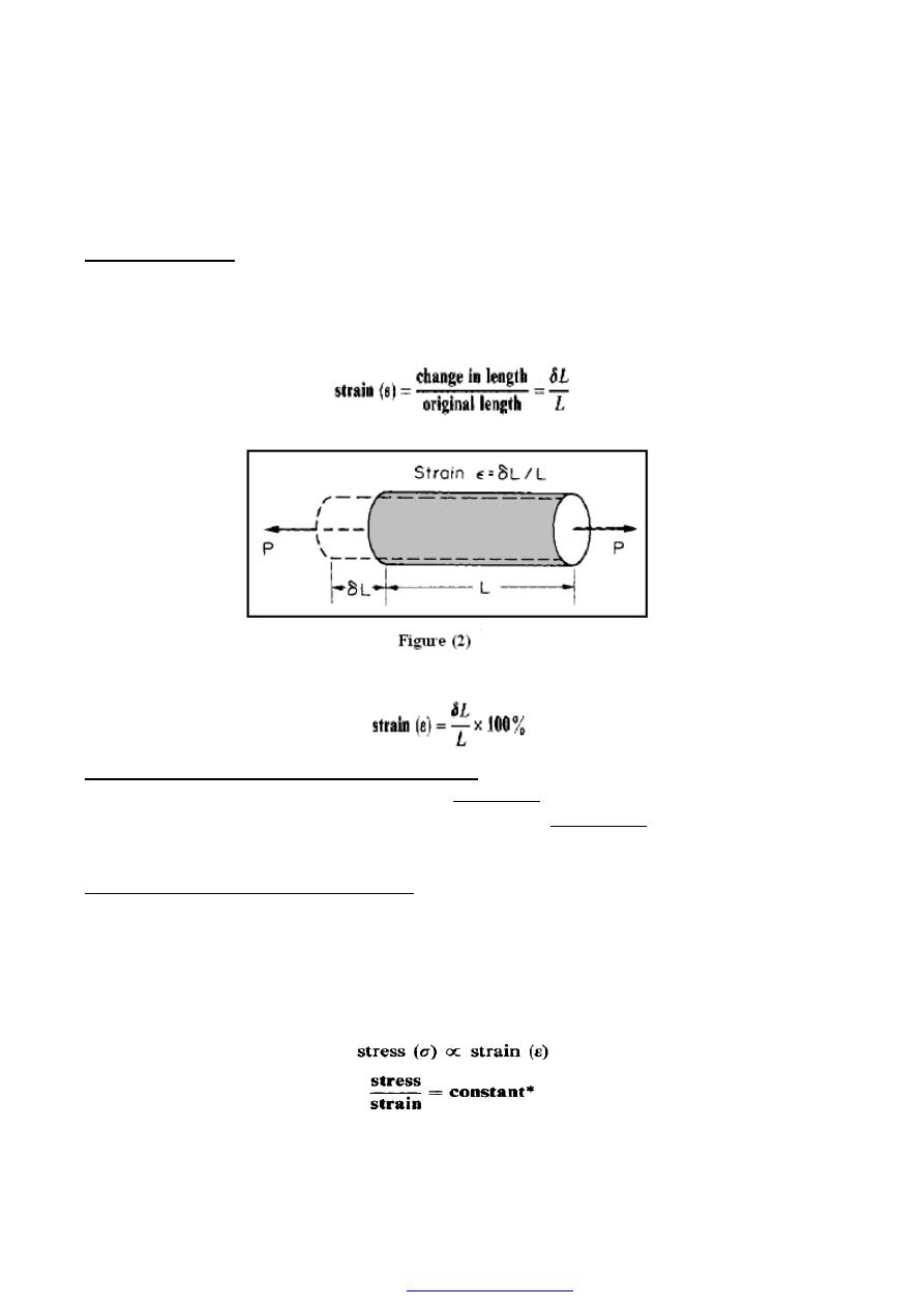
3. Direct strain (
ε
)
Figure (2) show a bar is subjected to a direct load, and hence a stress, the bar will change
in length. If the bar has an original length L and changes in length by an amount
δL, the
strain produced is defined as follows:
Strain is thus a measure of the deformation of the material and is non-dimensional,
Alternatively, strain can be expressed as a percentage strain
4. Sign convention for direct stress and strain
Tensile stresses and strains are considered
POSITIVE
in sense producing an increase in
length. Compressive stresses and strains are considered
NEGATIVE
in sense producing a
decrease in length.
5. Elastic materials - Hooke’s law (E), (N/m
2
)
A material is said to be elastic if it returns to its original, unloaded dimensions when
load is removed. A particular form of elasticity which applies to a large range of
engineering materials, at least over part of their load range, produces deformations which
are proportional to the loads producing them. stress is proportional to strain. Hooke
’s
law, in its simplest form*, therefore states that
PDF created with pdfFactory Pro trial version

4
Other classifications of materials with which the reader should be acquainted are as
follows:
A material which has a uniform structure throughout without any flaws or
discontinuities
is
termed
a
homogeneous
material.
Non-homogeneous
or
inhomogeneous materials such as concrete and poor-quality cast iron will thus have a
structure which varies from point to point depending on its constituents and the presence
of casting flaws or impurities.
If a material exhibits uniform properties throughout in all directions it is said to be
isotropic; conversely one which does not exhibit this uniform behaviour is said to be
nonisotropic or anisotropic.
An orthotropic material is one which has different properties in different planes. A
typical example of such a material is wood, although some composites which contain
systematically orientated “inhomogeneities” may also be considered to fall into this
category.
6. Modulus of elasticity - Young’s modulus (E), (N/m
2
)
Within the elastic limits of materials, i.e. within the limits in which Hooke’s law applies,
it has been shown that:
This constant is given the symbol E and termed the modulus of elasticity or Young
’s
modulus, Thus
ε
σ
=
=
Strain
Stress
E
…..(1)
L
A
L
P
E
δ
.
.
=
…..(2)
Young’s modulus E is generally assumed to be the same in tension or compression and
for most engineering materials has a high numerical value. Typically, E = 200 x l0
9
N/m
2
for steel.
E
σ
ε
=
……(3)
In most common engineering applications strains do not often exceed 0.003 or 0.3 % so
that the assumption used later in the text that deformations are small in relation to
original dimensions is generally well founded.
PDF created with pdfFactory Pro trial version
5
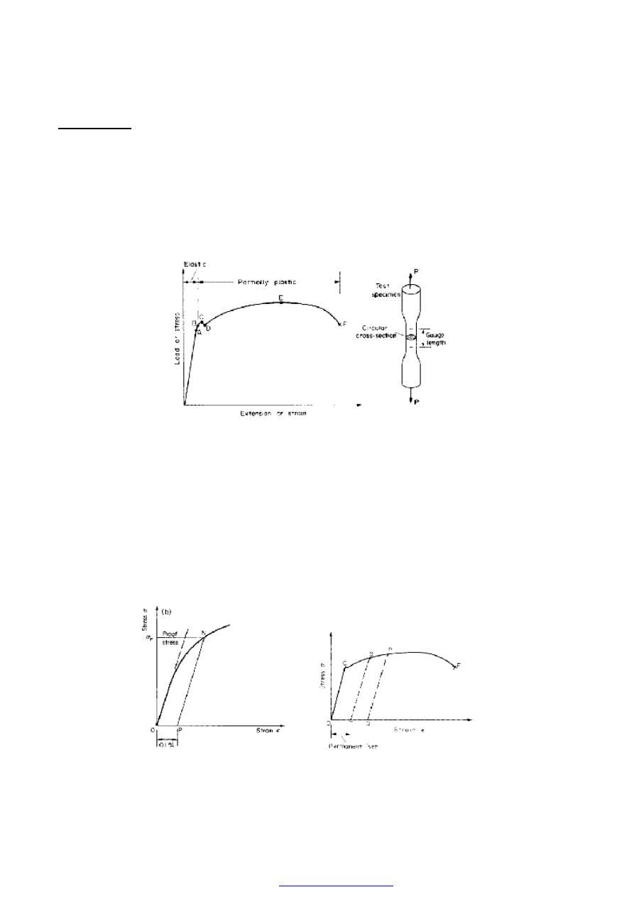
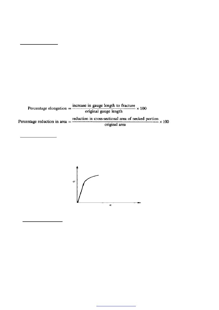
7. Tensile test
The standard tensile test in which a circular bar of uniform cross-section is subjected
to a gradually increasing tensile load until failure occurs. Measurements of the change in
length of a selected gauge length of the bar are recorded throughout the loading
operation by means of extensometers and a graph of load against extension or stress
against strain is produced as shown in Fig. (3); this shows a typical result for a test on a
mild (low carbon) steel bar; other materials will exhibit different graphs but of a similar
general form see Figures (5) to( 7).
Figure (3) Typical tensile test curve for mild steel.
For the first part of the test it will be observed that Hooke’s law is obeyed, the material
behaves elastically and stress is proportional to strain, giving the straight-line graph
indicated. Some point A is eventually reached, however, when the linear nature of the
graph ceases and this point is termed the limit of proportionality.
C, termed the upper yield point
D, the lower yield point
That stress which, when removed, produces a permanent strain or “set” of 0.1 % of the
original gauge length-see Fig. (4a).
Figure (4a) Determination of 0.1 % proof stress. Figure (4b) Permanent deformation or “set” after
straining beyond the yield point.
PDF created with pdfFactory Pro trial version
6
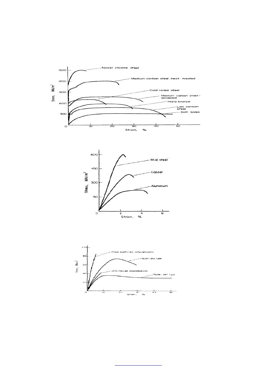
Typical stress-strain curves resulting from tensile tests on other engineering materials are
shown in Figs. (5) to (7).
Figure (5)Tensile test curves for various metals.
Figure (6) Typical stress - strain curves for hard drawn wire
material-note large reduction in strain values from those of Figure (5)
Figure(7) Typical tension test results for various types of
nylon and polycarbonate.
PDF created with pdfFactory Pro trial version
7
8. Ductile materials
It has been observed above that the partially plastic range of the graph of Figure (3)
covers a much wider part of the strain axis than does the elastic range. Thus the extension
of the material over this range is considerably in excess of that associated with elastic
loading. The capacity of a material to allow these large extensions, i.e. the ability to be
drawn out plastically, is termed its ductility. Materials with high ductility are termed
ductile materials, members with low ductility are termed brittle materials. A quantitative
value of the ductility is obtained by measurements of the percentage elongation or
percentage reduction in area, both
being defined below.
9. Brittle materials
A brittle material is one which exhibits relatively small extensions to fracture so that the
partially plastic region of the tensile test graph is much reduced (Fig. 8). Whilst Fig. (3)
referred to a low carbon steel, Fig. (8) could well refer to a much higher strength steel
with a higher carbon content. There is little or no necking at fracture for brittle materials.
Figure(8) Typical tensile test curve for a brittle material
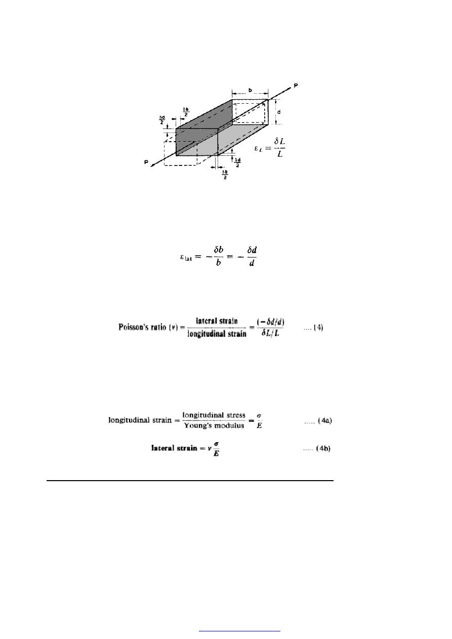
10. Poisson’s ratio (
ν)
Consider the rectangular bar of Figure (9) subjected to a tensile load. Under the action of
this load the bar will increase in length by an amount
δL giving a longitudinal strain in
the bar .
PDF created with pdfFactory Pro trial version
8
Figure (9)
The bar will also exhibit, however, a reduction in dimensions laterally, i.e. its breadth
and depth will both reduce. The associated lateral strains will both be equal, will be of
opposite sense to the longitudinal strain, and will be given by
Provided the load on the material is retained within the elastic range the ratio of the
lateral and longitudinal strains will always be constant. This ratio is termed Poisson
’s
ratio.
The negative sign of the lateral strain is normally ignored to leave Poisson’s ratio simply
as a ratio of strain magnitudes. It must be remembered, however, that the longitudinal
strain induces a lateral strain of opposite sign. For most engineering materials the value
of v lies between 0.25 and 0.33.
Since
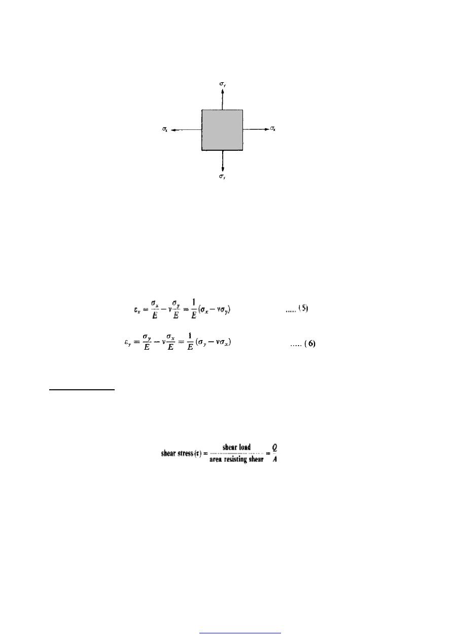
11. Application of Poisson’s ratio to a two-dimensional stress system
A two-dimensional stress system is one in which all the stresses lie within one plane such
as the X-Y plane as shown in figure (10).
PDF created with pdfFactory Pro trial version
9
Figure (10) Simple two-dimensional system of direct stresses.
The following strains will be produced
(a) in the X direction resulting from
ε
x
=
σ
x
/E
(b) in the Y direction resulting from
ε
y
=
σ
y
/E.
(c) in the X direction resulting from
ε
y
= - v(
σ
y
/E),
(d) in the Y direction resulting from
ε
x
= - v(
σ
x
/E).
strains (c) and (d) being the so-called Poisson
’s ratio strain, opposite in sign to the
applied strains, i.e. compressive.
The total strain in the X direction will therefore be given by
:
and the total strain in the Y direction will be:
If any stress is, in fact, compressive its value must be substituted in the above equations
together with a negative sign following the normal sign convention.
12. Shear stress(
τ
) , (N/m
2
)
Consider a block or portion of material as shown in Figure (11) subjected to a set of
equal and opposite forces Q. (Such a system could be realised in a bicycle brake block
when contacted with the wheel.) then a shear stress
τ is set up, defined as follows:
This shear stress will always be tangential to the area on which it acts; direct stresses,
however, are always normal to the area on which they act.
PDF created with pdfFactory Pro trial version
10
Figure(11) Shear force and resulting shear stress system showing typical form of failure by
relative sliding of planes.
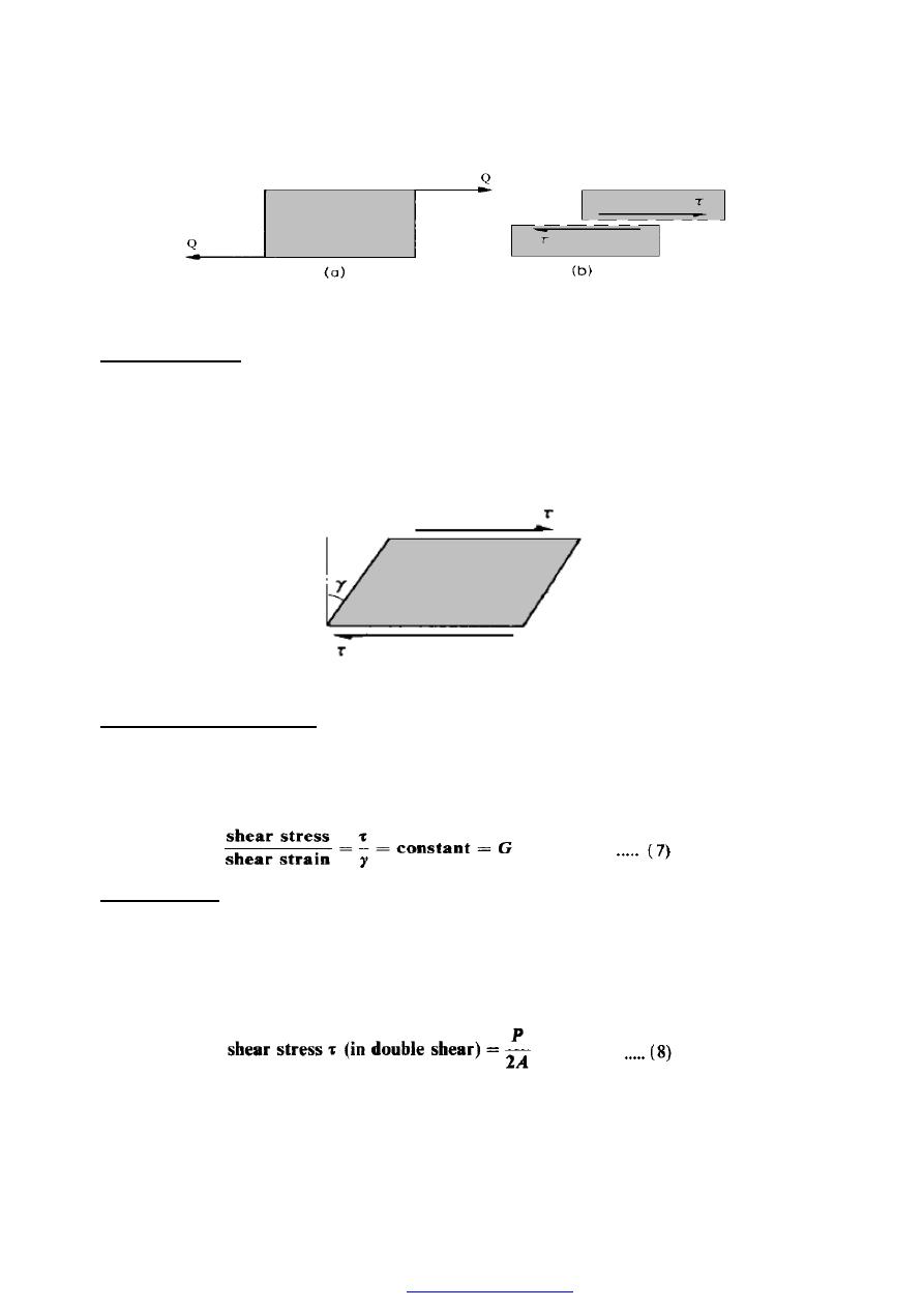
13. Shear strain (
γ
)
If one again considers the block of Figure (11a)to be a bicycle brake block it is clear that
the rectangular shape of the block will not be retained as the brake is applied and the
shear forces introduced. The block will in fact change shape or “strain” into the form
shown in Figure (12) The angle of deformation y is then termed the shear strain.
Shear strain is measured in radians and hence is non-dimensional, i.e. it has no units
.
Figure (12) Deformation (shear strain) produced by shear stresses.
14. Modulus of rigidity (G), (N/m
2
)
For materials within the elastic range the shear strain is proportional to the shear
stress producing it, The constant G is termed the modulus of rigidity or shear modulus
and is directly comparable to the modulus of elasticity used in the direct stress
application.
15. Double shear
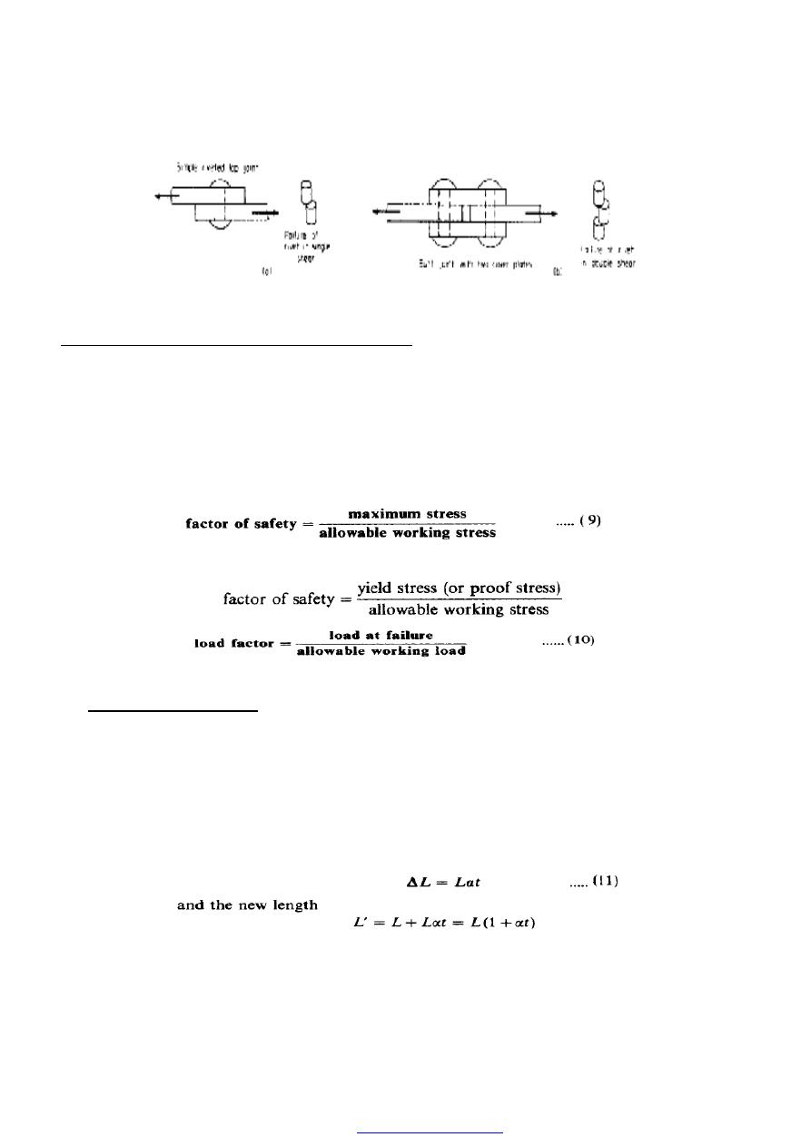
Consider the simple riveted lap joint shown in Figure (13a) When load is applied to
the plates the rivet is subjected to shear forces tending to shear it on one plane as
indicated. In the butt joint with two cover plates of Figure (13b), however, each rivet is
subjected to possible shearing on two faces, i.e. double shear. In such cases twice the
area
of metal is
resisting the applied forces so that the shear stress set up is given by
PDF created with pdfFactory Pro trial version
11
Figure (13) (a) Single shear. (b) Double shear.
16. Allowable working stress-factor of safety
The most suitable strength or stiffness criterion for any structural element or component
is normally some maximum stress or deformation which must not be exceeded. In the
case of stresses the value is generally known as the maximum allowable working stress.
Because of uncertainties of loading conditions, design procedures, production methods,
etc., designers generally introduce a factor of safety into their designs, defined as follows
:
18. Temperature stresses
When the temperature of a component is increased or decreased the material
respectively expands or contracts. If this expansion or contraction is not resisted in any
way then the processes take place free of stress. If, however, the changes in dimensions
are restricted then stresses termed temperature stresses will be set up within the material.
Consider a bar of material with a linear coefficient of expansion
α
. Let the original length
of the bar be L and let the temperature increase be t. If the bar is free to expand the
change in length would be given by
PDF created with pdfFactory Pro trial version
12
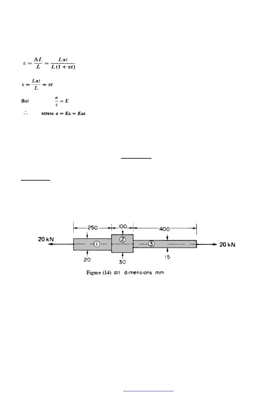
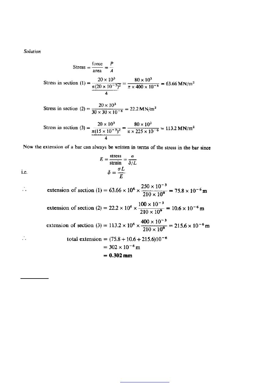
Examples
Example 1
Determine the stress in each section of the bar shown in Figure (14) when subjected to
an axial tensile load of 20 kN. The central section is 30 mm square cross-section; the
other portions are of circular section, their diameters being indicated. What will be the
total extension of the bar? For the bar material E = 210GN/m
2
.
PDF created with pdfFactory Pro trial version
13
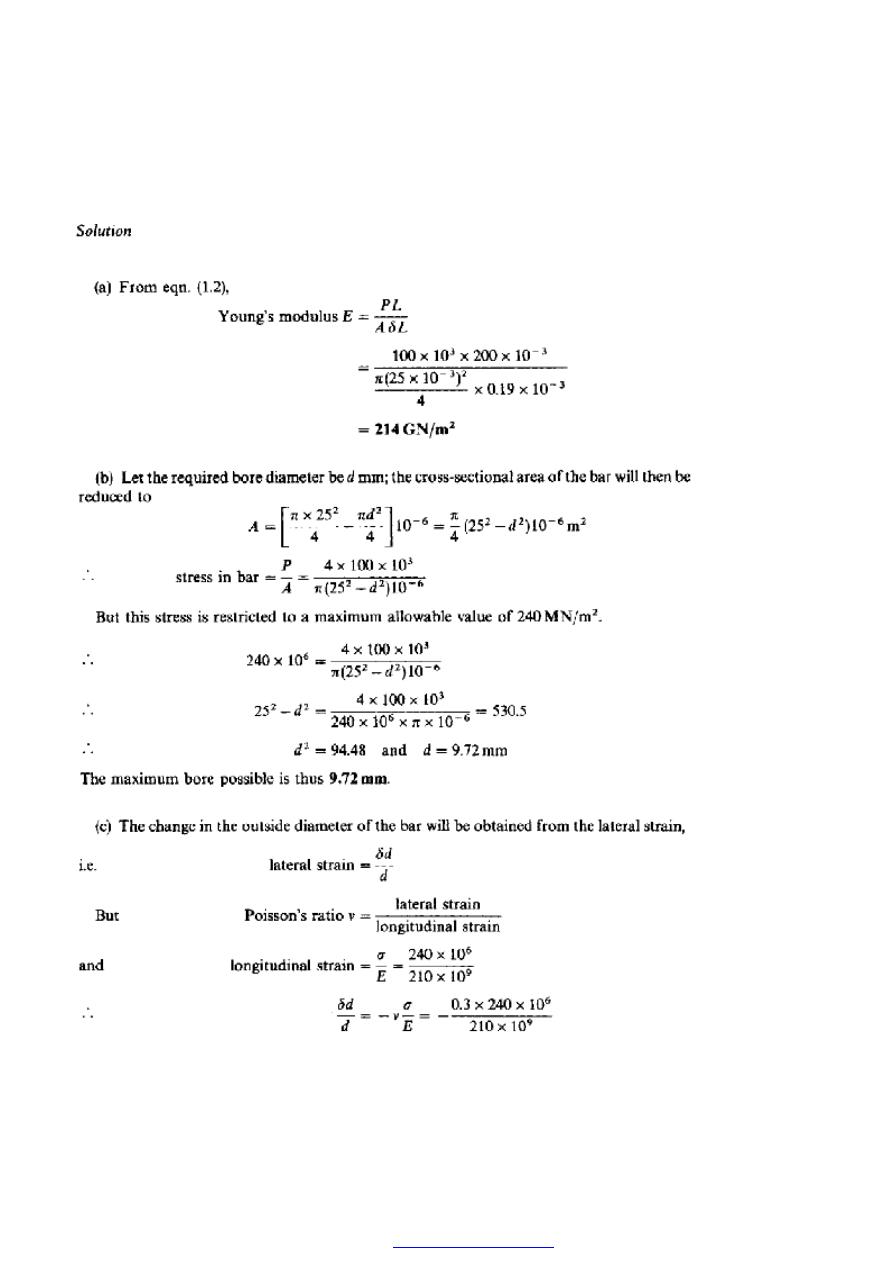
Example 2
(a) A 25 mm diameter bar is subjected to an axial tensile load of 100 kN. Under the
action of this load a 200mm gauge length is found to extend 0.19 x 10
-3
mm. Determine
the modulus of elasticity for the bar material.
(b) If, in order to reduce weight whilst keeping the external diameter constant, the bar is
bored axially to produce a cylinder of uniform thickness, what is the maximum diameter
of bore possible given that the maximum allowable stress is 240MN/m
2
? The load can be
assumed to remain constant at 100 kN.
PDF created with pdfFactory Pro trial version
14
(c) What will be the change in the outside diameter of the bar under the limiting stress
quoted in (b)? (E = 210GN/m2 and v = 0.3).
PDF created with pdfFactory Pro trial version

15
Example 3
The coupling shown in Figure (15) is constructed from steel of rectangular cross-section
and is designed to transmit a tensile force of 50 kN. If the bolt is of 15 mm diameter
calculate:
(a) the shear stress in the bolt;
(b) the direct stress in the plate;
(c) the direct stress in the forked end of the coupling
.
PDF created with pdfFactory Pro trial version
16
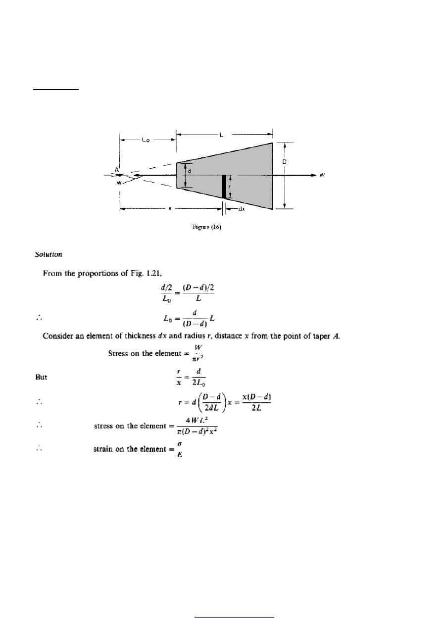
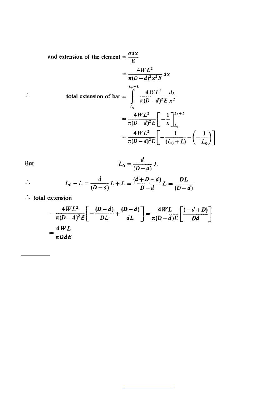
Example 4
Derive an expression for the total extension of the tapered bar of circular cross-section
shown in Figure (16) when it is subjected to an axial tensile load W.
PDF created with pdfFactory Pro trial version
17
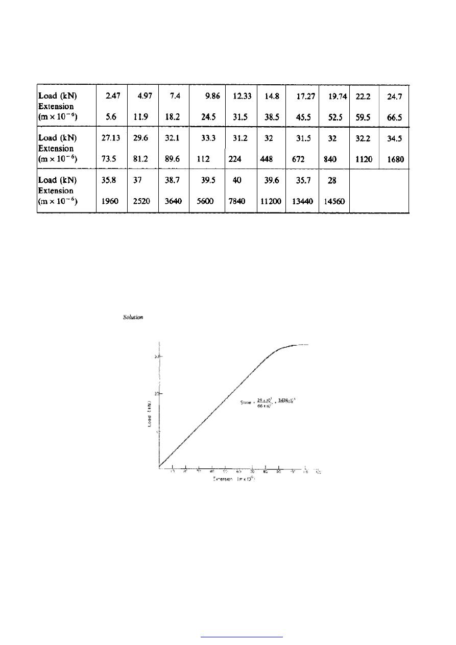
Example 5
The following figures were obtained in a standard tensile test on a specimen of low
carbon steel:
diameter of specimen, 11.28 mm;
gauge length, 56mm;
minimum diameter after fracture, 6.45 mm.
Using the above information and the table of results below, produce:
(1) a load/extension graph over the complete test range;
(2) a load/extension graph to an enlarged scale over the elastic range of the specimen.
PDF created with pdfFactory Pro trial version
18
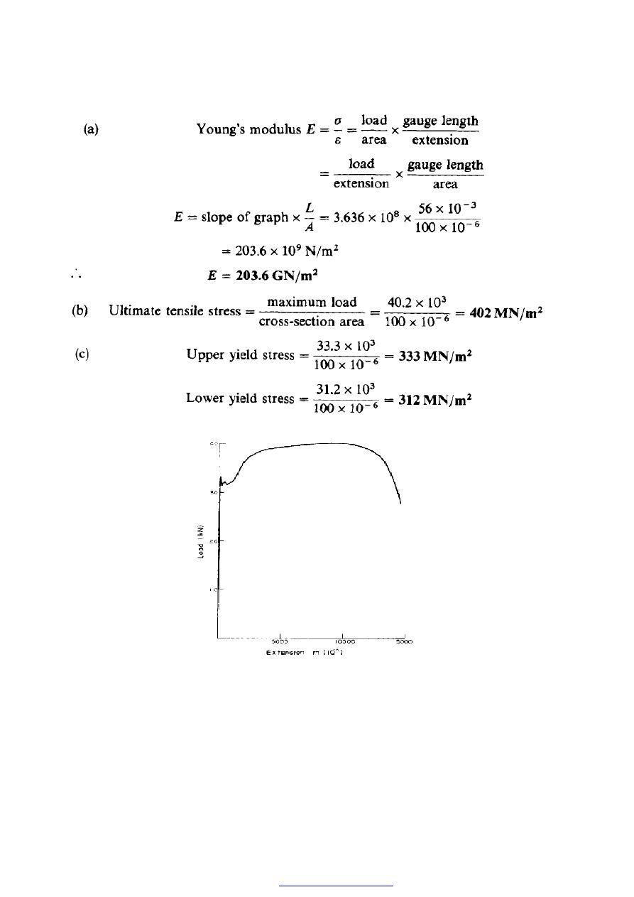
Using the two graphs and other information supplied, determine the values of
(a) Young's modulus of elasticity;
(b) the ultimate tensile stress;
(c) the stress at the upper and lower yield points;
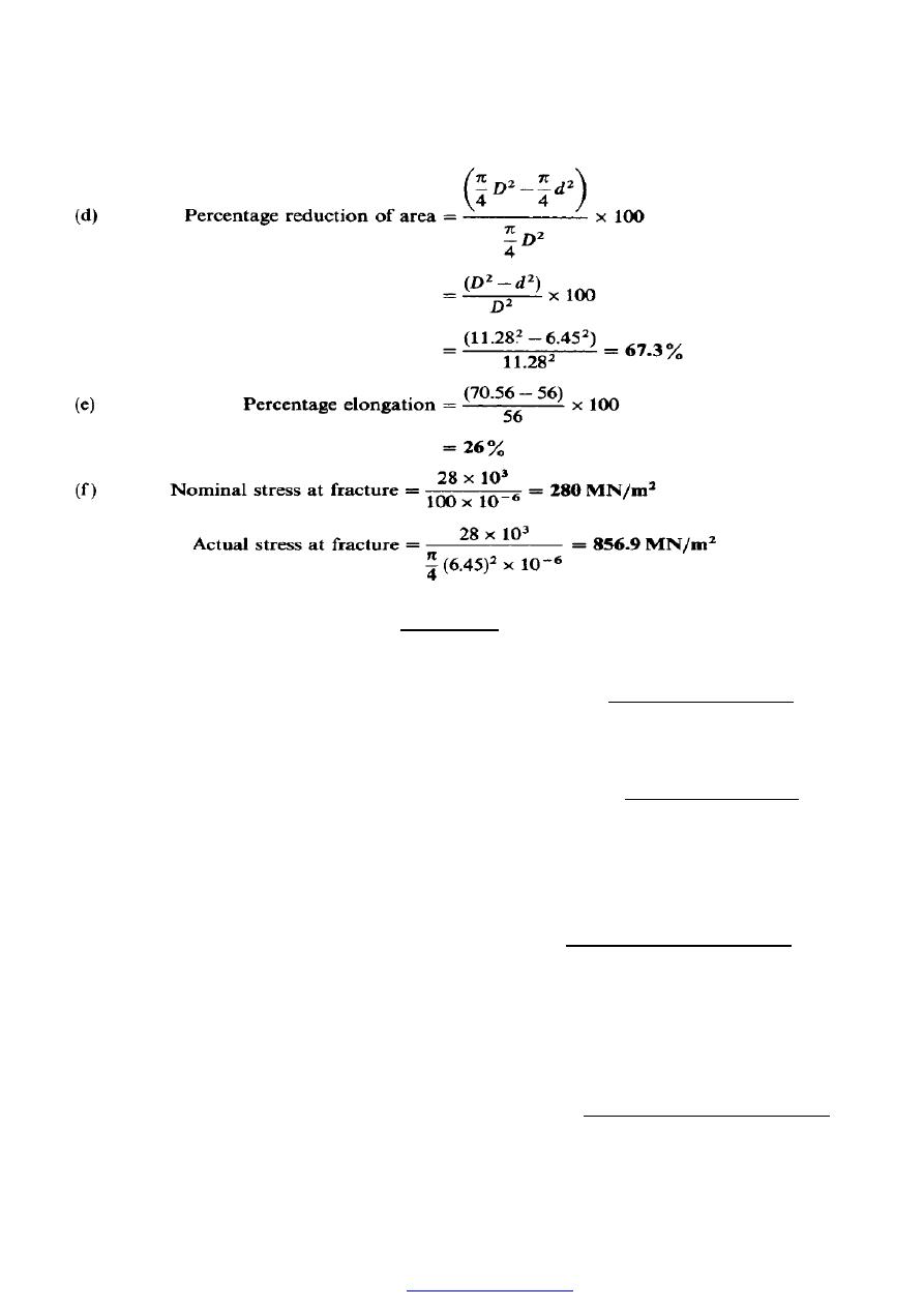
(d) the percentage reduction of area;
(e) the percentage elongation;
(f) the nominal and actual stress at fracture.
Figure (17) Load-extension graph for elastic range.
PDF created with pdfFactory Pro trial version
20
Problems
1. (A). A 25mm square cross-section bar of length 300mm carries an axial compressive
load of 50kN. Determine the stress set up in the bar and its change of length when the
load is applied. For the bar material E = 200 GN/m
2
. [80 MN/m
2
; 0.12mm]
2. (A). A steel tube, 25 mm outside diameter and 12mm inside diameter, cames an axial
tensile load of 40 kN. What will be the stress in the bar? What further increase in load
is possible if the stress in the bar is limited to 225 MN/m
2
? [l06 MN/m
2
; 45 kN]
3. (A). Define the terms shear stress and shear strain, illustrating your answer by means
of a simple sketch. Two circular bars, one of brass and the other of steel, are to be
loaded by a shear load of 30 kN. Determine the necessary diameter of the bars (a) in
single shear, (b) in double shear, if the shear stress in the two materials must not
exceed 50 MN/m
2
and 100 MN/m
2
respectively. [27.6, 19.5, 19.5, 13.8mm]
4. (A). Two forkend pieces are to be joined together by a single steel pin of 25mm
diameter and they are required to transmit 50 kN. Determine the minimum cross-
sectional area of material required in one branch of either fork if the stress in the fork
material is not to exceed 180 MN/m
2
. What will be the maximum shear stress in the
pin?
[1.39 x 10
-4
m
2
; 50.9MN/m
2
.]
PDF created with pdfFactory Pro trial version
21
5. (A). A simple turnbuckle arrangement is constructed from a 40 mm outside diameter
tube threaded internally at each end to take two rods of 25 mm outside diameter with
threaded ends. What will be the nominal stresses set up in the tube and the rods,
ignoring thread depth, when the turnbuckle cames an axial load of 30 kN? Assuming
a sufficient strength of thread, what maximum load can be transmitted by the
turnbuckle if the maximum stress is limited to 180 MN/m
2
?
[39.2, 61.1 MN/m2, 88.4 kN]
6. (A). A bar ABCD consists of three sections: AB is 25 mm square and 50 mm long, BC
is of 20 mm diameter and40 mm long and CD is of 12 mm diameter and 50 mm long.
Determine the stress set up in each section of the bar when it is subjected to an axial
tensile load of 20 kN. What will be the total extension of the bar under this load? For
the bar material, E = 210GN/m
2
. [32,63.7, 176.8 MN/m
2
, 0.062mm]
7.(A). A steel bar ABCD consists of three sections: AB is of 20mm diameter and 200
mm long, BC is 25 mm square and 400 mm long, and CD is of 12 mm diameter and
200mm long. The bar is subjected to an axial compressive load which induces a stress
of 30 MN/m
2
on the largest cross-section. Determine the total decrease in the length of
the bar when the load is applied. For steel E = 210GN/m
2
.
[0.272 mm.]
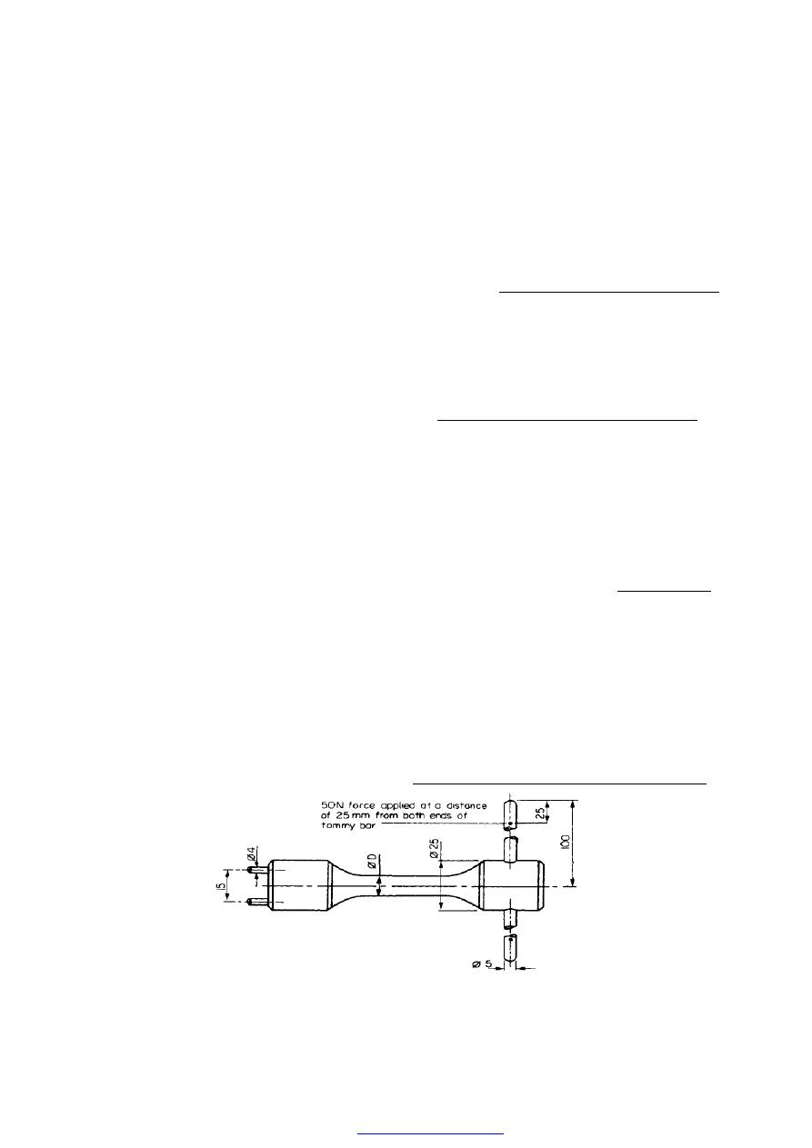
8. Figure (19) shows a special spanner used to tighten screwed components. A torque is
applied at the tommy -bar and is transmitted to the pins which engage into holes
located into the end of a screwed component.
(a) Using the data given in Figure (19) calculate:
(i) the diameter D of the shank if the shear stress is not to exceed 50N/mm
2
,
(ii) the stress due to bending in the tommy-bar,
(iii) the shear stress in the pins.
[9.14mm; 254.6 MN/m
2
; 39.8 MN/m
2
.]
Figure (19)
PDF created with pdfFactory Pro trial version
22
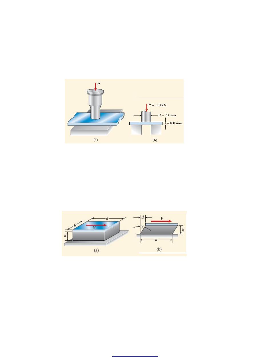
Q9-A punch for making holes in steel plates is shown in Figure (1a). Assume that a
punch having diameter d =20 mm is used to punch a hole in an 8-mm plate, as
shown in the cross-sectional view Figure (1b). If a force P= 110 kN is required to
create the hole, what is the average shear stress in the plate and the average
compressive stress in the punch?
Figure (1)
Q10-A bearing pad of the kind used to support machines and bridge girders consists of a
linearly elastic material (usually an elastomer, such as rubber) capped by a steel
plate Figure (2a). Assume that the thickness of the elastomer is h, the dimensions of
the plate are (a . b), and the pad is subjected to a horizontal shear force V. Obtain
formulas for the average shear stress (
τ
) in the elastomer and the horizontal
displacement d of the plate Figure (2b).
Figure (2)
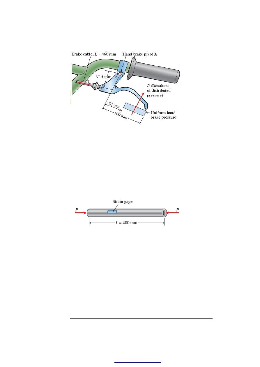
Q11-A force P of 70 N is applied by a rider to the front hand brake of a bicycle (P is the
resultant of an evenly distributed pressure). As the hand brake pivots at A, a tension T
develops in the 460-mm long brake cable (Ae =1.075 mm
2
) which elongates by
δ
= 0.214
mm. Find normal stress (
σ
) and strain (
ε
) in the brake cable.
PDF created with pdfFactory Pro trial version
23
Figure (3)
Q12-A circular aluminum tube of length L = 400 mm is loaded in compression by forces
P Figure (4). The outside and inside diameters are 60 mm and 50 mm, respectively. A
strain gage is placed on the outside of the bar to measure normal strains in the
longitudinal direction.
(a) If the measured strain is
ε
= 550 x 10
-6
, what is the shortening
δ
of the bar?
(b) If the compressive stress in the bar is intended to be 40 MPa, what should be the load
P?
Figure (4)
Q13-(a) A test piece is cut from a brass bar and subjected to a tensile test. With a load of
6.4 kN the test piece, of diameter 11.28 mm, extends by 0.04 mm over a gauge length of
50 mm. Determine:
(i) the stress, (ii) the strain, (iii) the modulus of elasticity.
(b) A spacer is turned from the same bar. The spacer has a diameter of 28 mm and a
length of 250mm. both measurements being made at 20°C. The temperature of the spacer
is then increased to 100°C, the natural expansion
being entirely prevented. Taking the coefficient of linear expansion to be18 x 10
-6
/
o
C
determine:
(i) the stress in the spacer, (ii) the compressive load on the spacer.
Ans. [64MN/m
2
, 0.0008, 80GN/m
2
, 115.2 MN/m
2
, 71 kN.]
PDF created with pdfFactory Pro trial version
24
COMPOUND BARS
1. Compound bars subjected to external load
In certain applications it is necessary to use a combination of elements or bars made
from different materials. In overhead electric cables, for example, it is often convenient to
carry the current in a set of copper wires surrounding steel wires, the latter being
designed to support the weight of the cable over large spans. Such combinations of
materials are generally termed compound burs. This chapter is concerned with compound
bars which are symmetrically proportioned such that no bending results, when an external
load is applied to such a compound bar it is shared between the individual component
materials in proportions depending on their respective lengths, areas and Young’s
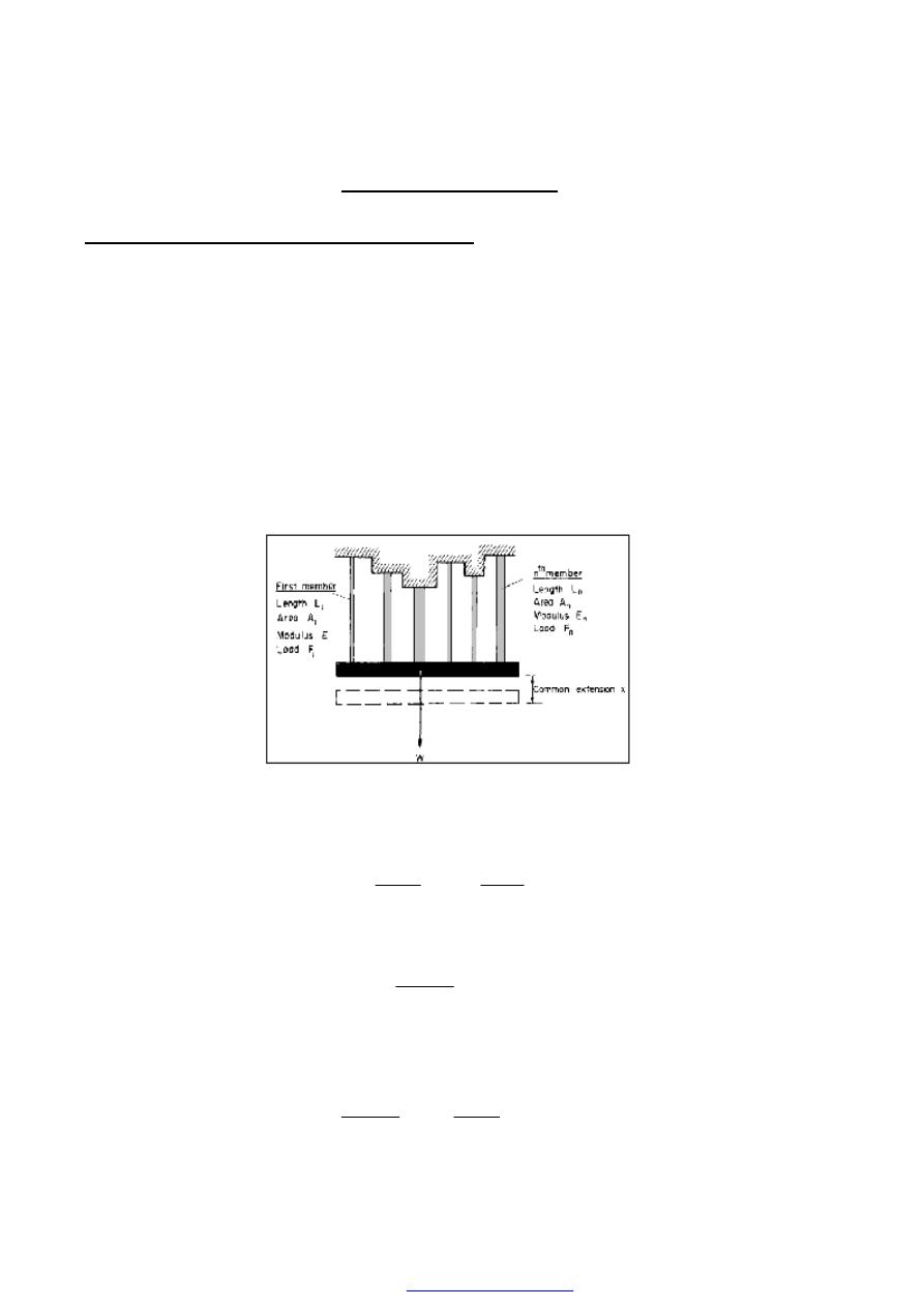
moduli. A compound bar consisting of n members, each having a different
length and cross-sectional area and each being of a different material as shown in figure
(1)
Figure (1) Compound bar formed of different materials
For the nth member,
n
n
n
n
n
x
A
L
F
E
strain
stress
.
.
=
=
n
n
n
n
L
x
A
E
F
.
.
=
....(1)
where F, is the force in the nth member ,A its cross-sectional area and
n
L
are its
length. The total load carried will be the sum of all such loads for all the members
∑
∑
=
=
n
n
n
n
n
n
L
A
E
x
L
x
A
E
W
.
.
.
.
...(2)
PDF created with pdfFactory Pro trial version
25
Now from equation (1) the force in member 1 is given by
1
1
1
1
.
.
L
x
A
E
F
=
But, from equation (2),
∑
=
n
n
n
L
A
E
W
x
.
W
L
A
E
L
A
E
F
∑
=
.
.
1
1
1
1
.....(3)
i
.e. each member carries a portion of the total load W proportional to its EAIL value. If
the wires are all of equal length the above equation reduces to
W
A
E
A
E
F
∑
=
.
.
1
1
1
....(4)
The stress in member 1 is then given by
1
1
1
A
F
=
σ
....(5)
2. Compound bars - “equivalent” or “combined” modulus
In order to determine the common extension of a compound bar it is convenient to
consider it as a single bar of an imaginary material with an equivalent or combined
modulus E,. Here it is necessary to assume that both the extension and the original
lengths of the individual members of the compound bar are the same; the strains in all
members will then be equal.
Now total load on compound bar = F
1
+ F
2
+ F
3
+ . . . + F, where F
1
, F
2
, etc., are the
loads in members 1, 2, etc.
But
force = stress x area
n
n
n
A
A
A
A
A
A
σ
σ
σ
σ
+
+
+
=
+
+
+
......
)
......
(
2
2
1
1
2
1
Where:
σ is the stress in the equivalent single bar. Dividing through by the common
strain
ε,
PDF created with pdfFactory Pro trial version

26
n
n
n
A
A
A
A
A
A
ε
σ
ε
σ
ε
σ
ε
σ
+
+
+
=
+
+
+
......
)
.......
(
2
2
1
1
2
1
n
n
n
c
A
E
A
E
A
E
A
A
A
E
+
+
+
=
+
+
+
.......
)
......
(
2
2
1
1
2
1
where
c
E
, is the equivalent or combined E of the single bar.
n
A
A
A
n
A
n
E
A
E
A
E
E
combined
+
+
+
+
+
+
=
...
2
1
.
....
2
.
2
1
.
1
∑
∑
=
A
A
E
E
c
.
....(6)
With an external load W applied,
∑
=
A
W
bar
equivalent
the
in
Stress
L
x
A
E
W
bar
equivalent
the
in
Strain
c
=
=
∑
.
∑
=
A
E
L
W
x
extension
common
c
.
.
....(7)
=extension of single bar
3. Compound bars subjected to temperature change
When a material is subjected to a change in temperature its length will change by an
amount
T
L
∆
.
.
α
where
α is the coefficient of linear expansion for the material, L is the original length and
T
∆
the temperature change. (An increase in temperature produces an increase in length
and a decrease in temperature a decrease in length except in very special cases of
materials with zero or negative coefficients of expansion which need not be considered
here.) If, however, the free expansion of the material is prevented by some external force,
then a stress is set up in the material. This stress is equal in magnitude to that which
would be produced in the bar by initially allowing the free change of length and then
applying sufficient force to return the bar to its original length.
Now:
PDF created with pdfFactory Pro trial version
27
T
L
Length
in
Change
∆
=
.
.
α
T
L
T
L
Strain
∆
=
∆
=
.
.
.
α
α
Therefore, the stress created in the material by the application of sufficient force to
remove this strain
T
E
E
x
strain
∆
=
=
.
.
α
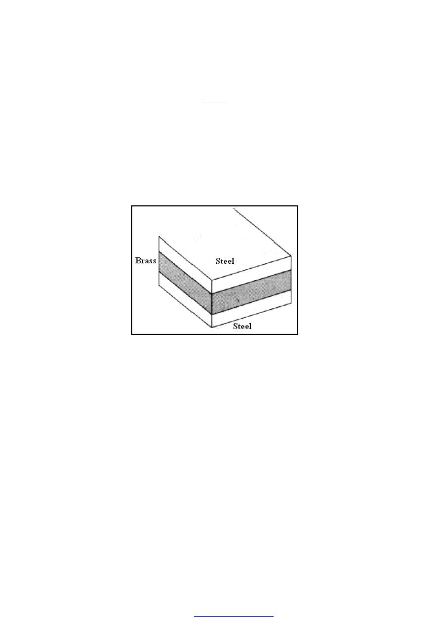
Consider now a compound bar constructed from two different materials rigidly joined
together as shown in Figure (2) and Figure (3a). For simplicity of description consider
that the materials in this case are steel and brass.
Figure (2)
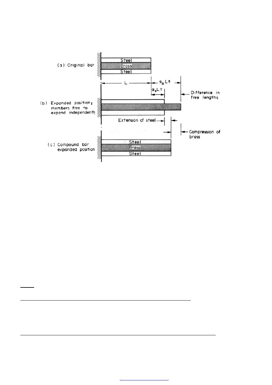
In general, the coefficients of expansion of the two materials forming the compound bar
will be different so that as the temperature rises each material will attempt to expand by
different amounts. Figure (3b) shows the positions to which the individual materials will
extend if they are completely free to expand (i.e. not joined rigidly together as a
compound bar). The extension of any length L is given by
T
L
∆
.
.
α
PDF created with pdfFactory Pro trial version
28
Figure (3) Thermal expansion of compound bar.
Thus the difference of "free" expansion lengths or so-called free lengths
T
L
T
L
T
L
s
B
s
B
∆
−
=
∆
−
∆
=
.
).
(
.
.
.
.
α
α
α
α
since in this case the coefficient of expansion of the brass
(
B
α
) is greater than that for
the steel (
s
α
). The initial lengths L of the two materials are assumed equal. If the two
materials are now rigidly joined as a compound bar and subjected to the same
temperature rise, each material will attempt to expand to its free length position but each
will be affected by the movement of the other, The higher coefficient of expansion
material (brass) will therefore seek to pull the steel up to its free length position and
conversely the lower position. In practice a compromise is reached, the compound bar
extending to the position shown in Figure (3c), resulting in an effective compression of
the brass from its free length position and an effective extension of the steel from its free
length position. From the diagram it will be seen that the following rule holds.
Rule 1
(Extension of steel + compression of brass = difference in “free” lengths).
Referring to the bars in their free expanded positions the rule may be written as
(Extension of “short” member + compression of“1ong” member = difference in free
lengths).
Applying Newton’s law of equal action and reaction the following second rule also applies.
PDF created with pdfFactory Pro trial version
29
Rule 2
The tensile force applied to the short member by the long member is equal in magnitude
to the compressive force applied to the long member by the short member.
Thus, in this case,
tensile force in steel = compressive force in brass
Now, from the definition of Young’s modulus
L
L
strain
stress
E
/
∆
=
=
σ
where
∆L is the change in length
.
E
L
L
.
σ
=
∆
Also,
force = stress x area =
σ.A
where: A is the cross-sectional area, Therefore Rule 1 becomes
T
L
E
L
E
L
s
B
B
B
s
s
∆
−
=
+
.
).
(
.
.
α
α
σ
σ
....(8)
and Rule 2 becomes
B
B
s
s
A
A
.
.
σ
σ
=
....(9)
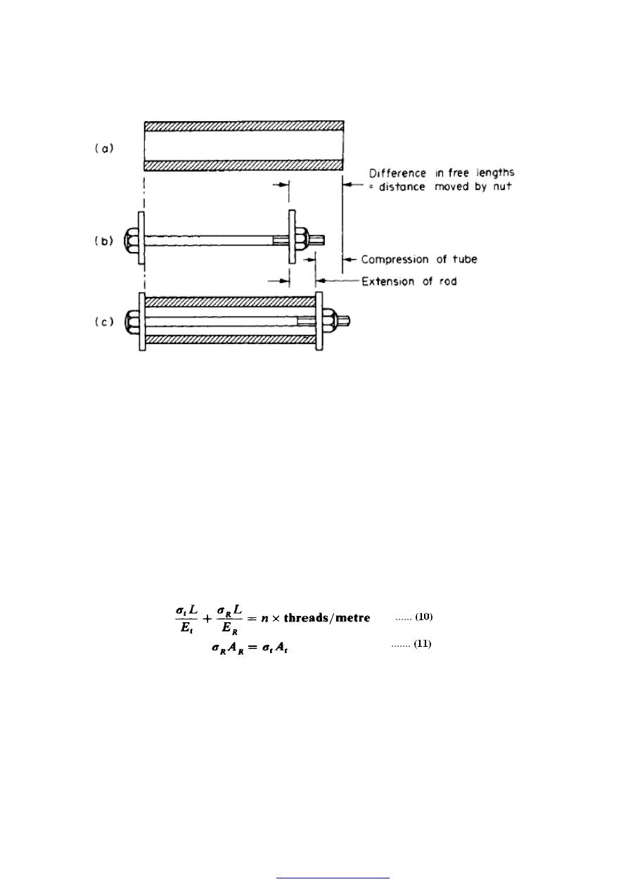
4. Compound bar (tube and rod)
Consider now the case of a hollow tube with washers or endplates at each end and a
central threaded rod as shown in Figure (4) At first sight there would seem to be no
connection with the work of the previous section, yet, in fact, the method of solution to
determine the stresses set up in the tube and rod when one nut is tightened.
The compound bar which is formed after assembly of the tube and rod, i.e. with the nuts
tightened, is shown in Figure (4c), the rod being in a state of tension and the tube in
compression. Once again Rule 2 applies, i.e.
compressive force in tube = tensile force in rod
PDF created with pdfFactory Pro trial version
30
Figure (4)
Figure (4a) and b show, diagrammatically, the effective positions of the tube and rod
before the nut is tightened and the two components are combined. As the nut is turned
there is a simultaneous compression of the tube and tension of the rod leading to the final
state shown in Figure ( 4c) . As before, however, the diagram shows that Rule 1 applies:
compression of tube +extension of rod = difference in free lengths
= axial advance of nut
i.e. the axial movement of the nut ( = number of turns n x threads per metre) is taken up
by combined compression of the tube and extension of the rod.
Thus, with suffix (t) for tube and (R) for rod,
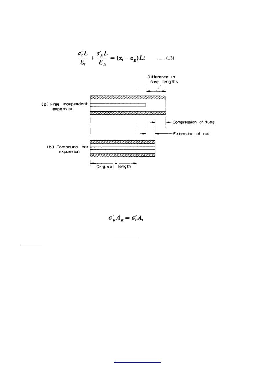
If the tube and rod are now subjected to a change of temperature they may be treated as a
normal compound bar and Rules 1 and 2 again apply
Figure (5),
PDF created with pdfFactory Pro trial version
31
Figure (5)
Where
(
/
R
σ )
;
and
(
/
R
σ
) ; are the stresses in the tube and rod due to temperature
change only and
(
t
α )
, is assumed greater than
(
R
α )
.
If the latter is not the case the two
terms inside the final bracket should be interchanged.
Also
Examples
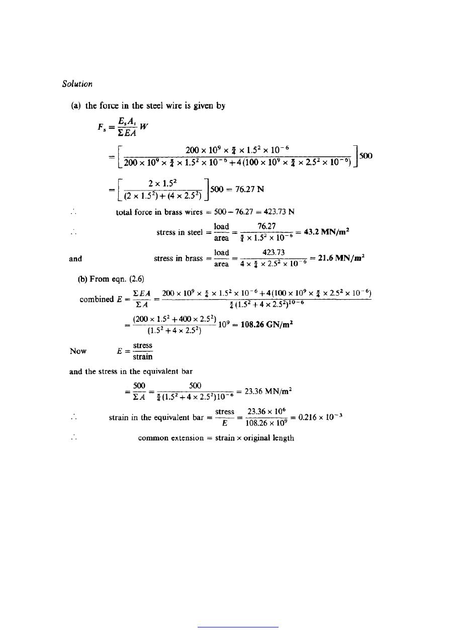
Example 1
(a) A compound bar consists of four brass wires of 2.5 mm diameter and one steel wire of
1.5 mm diameter. Determine the stresses in each of the wires when the bar supports a
load of 500 N. Assume all of the wires are of equal lengths.
(b) Calculate the “equivalent” or “combined modulus for the compound bar and
determine its total extension if it is initially 0.75 m long. Hence check the values of the
stresses obtained in part (a).
For brass E = 100 GN/m
2
and for steel E = 200 GN/m
2
.
PDF created with pdfFactory Pro trial version
33
Example 2
(a) A compound bar is constructed from three bars 50 mm wide by 12 mm thick
fastened together to form a bar 50 mm wide by 36 mm thick. The middle bar is of
aluminium alloy for which E = 70 GN/m
2
and the outside bars are of brass with E =
100 GN/m
2
. If the bars are initially fastened at 18°C and the temperature of the whole
assembly is then raised to 50
o
C, determine the stresses set up in the brass and the
aluminium.
B
α
= 18 x per
o
C and
A
α
= 22 x per
o
C
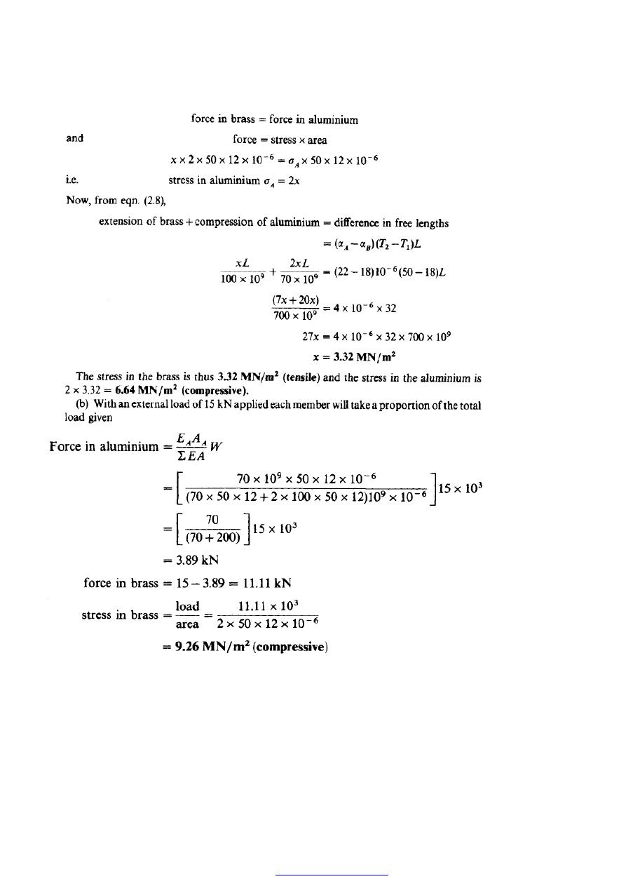
(b) What will be the changes in these stresses if an external compressive load of 15 kN is
applied to the compound bar at the higher temperature?
Solution
With any problem of this type it is convenient to let the stress in one of the component
members or materials, e.g. the brass, be x.
Then, since
PDF created with pdfFactory Pro trial version
34
These stresses represent the changes in the stresses owing to the applied load. The total or
resultant stresses owing to combined applied loading plus temperature effects are,
therefore,
PDF created with pdfFactory Pro trial version
35
Example 3
A 25 mm diameter steel rod passes concentrically through a bronze tube 400 mm long, 50
mm external diameter and 40 mm internal diameter. The ends of the steel rod are
threaded and provided with nuts and washers which are adjusted initially so that there is
no end play at 20°C.
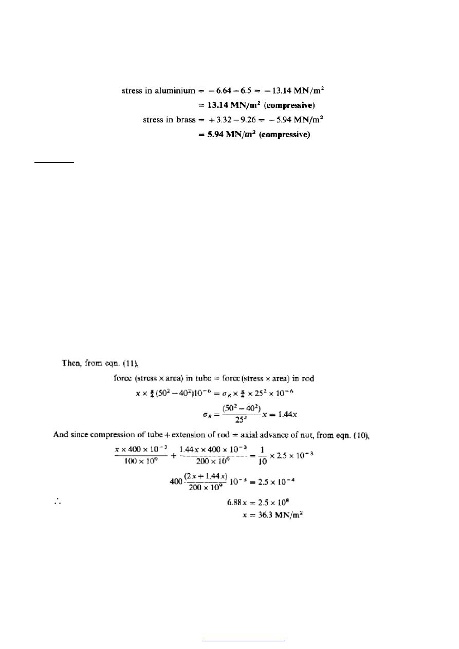
(a) Assuming that there is no change in the thickness of the washers, find the stress
produced in the steel and bronze when one of the nuts is tightened by giving it one tenth
of a turn, the pitch of the thread being 2.5 mm.
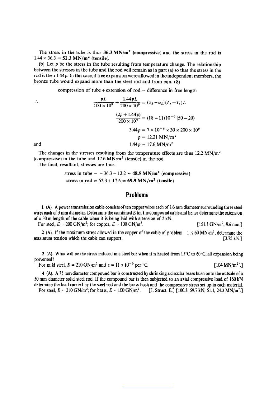
(b) If the temperature of the steel and bronze is then raised to 50°C find the changes that
will occur in the stresses in both materials.
The coefficient of linear expansion per
o
C is 11 x 10
-6
for steel and for bronze and 18 x10
-
6
. E for steel = 200 GN/m
2
. E for bronze = 100 GN/m
2
.
Solution
(a) Let x be the stress in the tube resulting from the tightening of the nut and
R
σ
the
stress in the rod
PDF created with pdfFactory Pro trial version
37
SHEARING FORCE AND BENDING MOMENT
DIAGRAMS
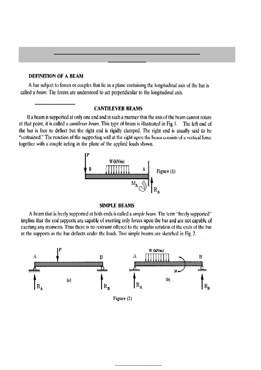
1. Types of Beams
PDF created with pdfFactory Pro trial version
38
2. Shearing force and bending moment
At every section in a beam carrying transverse loads there will be resultant forces on
either side of the section which, for equilibrium, must be equal and opposite, and whose
combined action tends to shear the section in one of the two ways shown in Figure (4 a
and b). The shearing force (S.F.) at the section is defined therefore as the algebraic sum
of the forces taken on one side of the section.
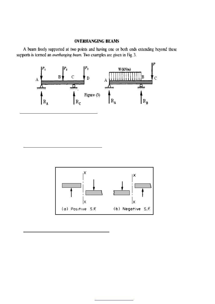
2.1. Shearing force (S.F.) sign convention
Forces upwards to the left of a section or downwards to the right of the section are
positive. Thus Figure (4a) shows a positive S.F. system at X-X and Figure (4b) shows a
negative S.F. system.
Figure (4) S.F. sign convention
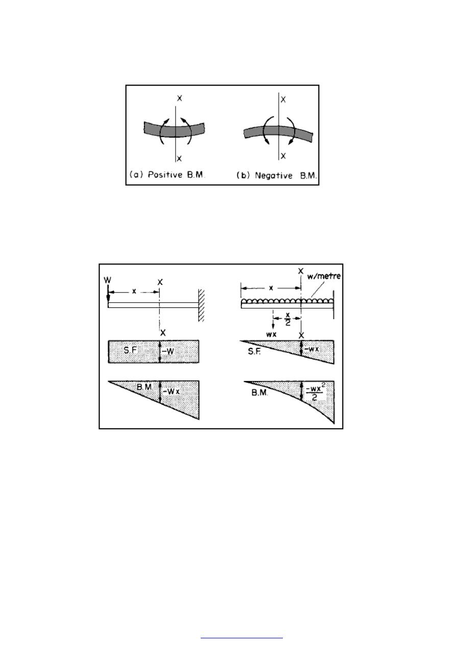
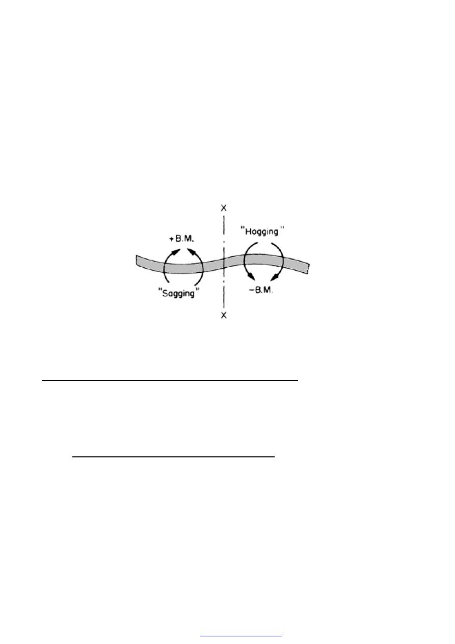
2.2. Bending moment (B.M.) sign convention
Clockwise moments to the left and counterclockwise to the right are positive. Thus
Figure (5a) shows a positive bending moment system resulting in sagging of the beam at
X-X and Figure (5b) illustrates a negative B.M. system with its associated hogging beam.
PDF created with pdfFactory Pro trial version
39
Figure (5) B.M. sign convention.
It should be noted that whilst the above sign conventions for S.F. and B.M. are somewhat
arbitrary and could be completely reversed, the systems chosen here are the only ones
which yield the mathematically correct signs for slopes and deflections of beams in
subsequent work and therefore are highly recommended.
Figure (6) S.F.-B.M. diagrams for standard cases.
Thus in the case of a cantilever carrying a concentrated load (W) at the end Figure (6),
the S.F. at any section X-X, distance x from the free end, is S.F. = - W. This will
be true whatever the value of x, and so the S.F. diagram becomes a rectangle. The B.M.
at the same section X-X is- W.x and this will increase linearly with x. The B.M. diagram
is therefore a triangle. If the cantilever now carries a uniformly distributed load, the S.F.
at X-X is the net load to one side of X-X, i.e. -wx. In this case, therefore, the S.F.
diagram becomes triangular, increasing to a maximum value of - WL at the support. The
B.M. at X-X is obtained by treating the load to the left of X-X as a concentrated load of
the same value acting at the centre of gravity,
PDF created with pdfFactory Pro trial version
40
Plotted against x this produces the parabolic B.M. diagram shown.
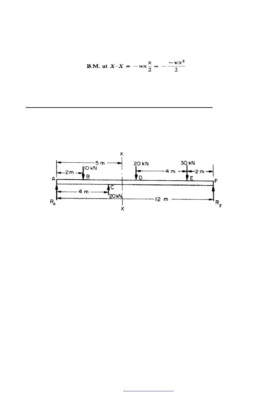
3. S.F. and B.M. diagrams for beams carrying concentrated loads only
In order to illustrate the procedure to be adopted for the determination of S.F. and B.M.
values for more complicated load conditions, consider the simply supported beam shown
in
Figure (4) carrying concentrated loads only. (The term simply supported means that the
beam can be assumed to rest on knife-edges or roller supports and is free to bend at the
supports without any restraint.)
Figure (7)
The values of the reactions at the ends of the beam may be calculated by applying normal
equilibrium conditions, i.e. by taking moments about F.
Thus
R
A
x 12 = (10 x 10) + (20 x 6) + (30 x 2) - (20 x 8) = 120
R
A
= 10 kN
For vertical equilibrium
total force up = total load down
R
A
+R
F
= 10+20+30-20 = 40
R
F
= 30 kN
At this stage it is advisable to check the value of RF by taking moments about A.
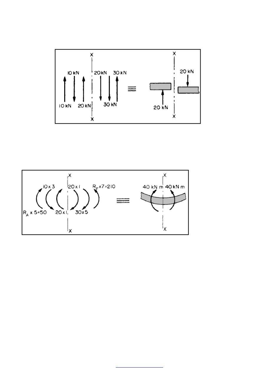
Summing up the forces on either side of X-X we have the result shown in Figure (8)
Using the sign convention listed above, the shear force at X-X is therefore +20kN,i.e the
resultant force at X-X tending to shear the beam is 20 kN.
PDF created with pdfFactory Pro trial version
41
Figure (8) Total S.F. at X-X.
Similarly, Figure (9) shows the summation of the moments of the forces at X-X, the
resultant B.M. being 40 kNm.
Figure (9)
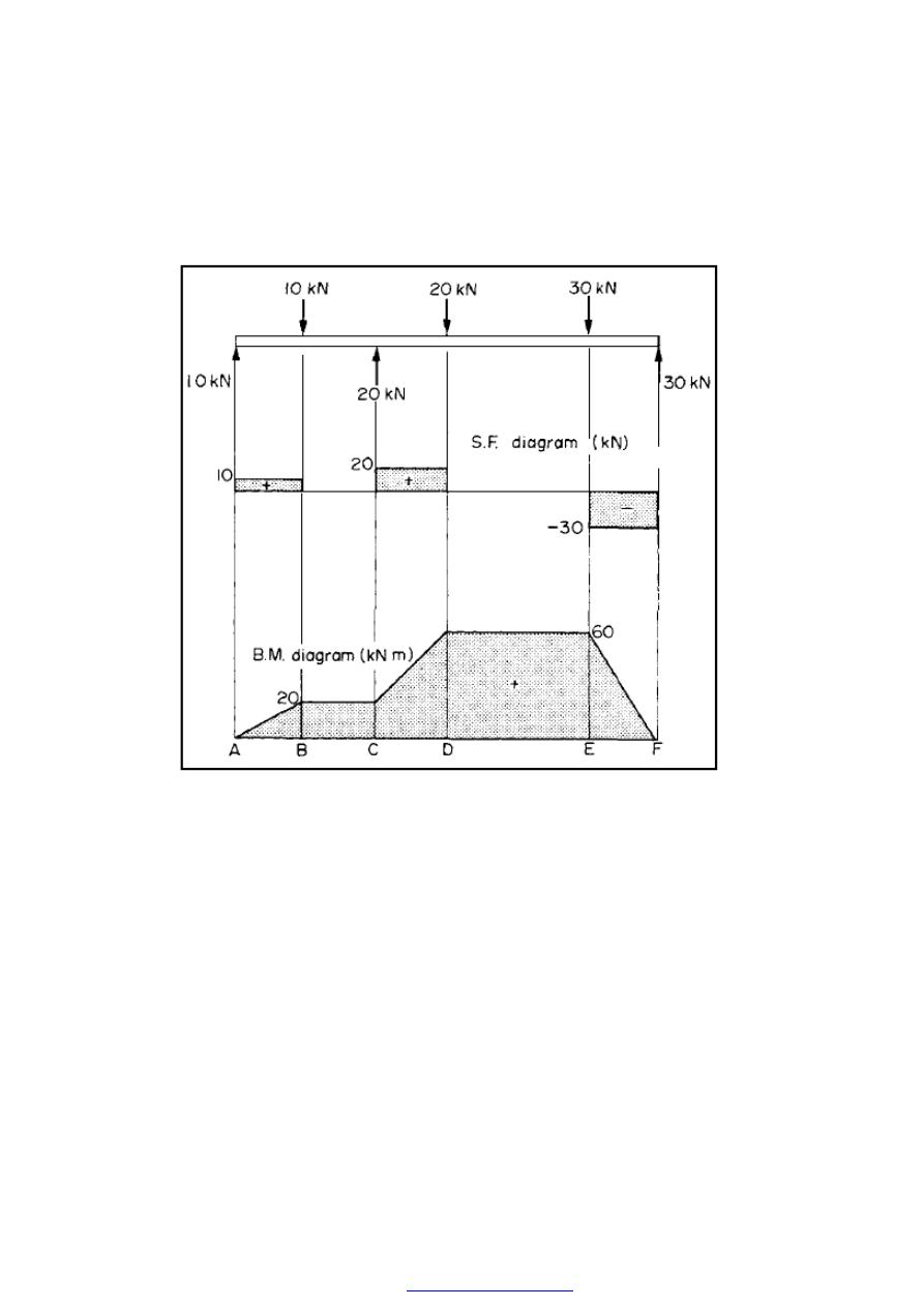
In practice only one side of the section is normally considered and the summations
involved can often be completed by mental arithmetic. The complete S.F. and B.M.
diagrams for the beam are shown in Figure (9).
B.M. at A = o
B.M. at B = + (10 x 2) = +20 kN.m
B.M. at C= +(l0 x 4)-(10 x 2) = +20kN.m
B.M. at D = +(l0 x 6)+ (20 x 2)- (10 x 4) = +60 kN.m
B.M. at E = + (30 x 2) = +60 kN.m
B.M. at F = 0
PDF created with pdfFactory Pro trial version
42
All the above values have been calculated from the moments of the forces to the left of
each section considered except for E where forces to the right of the section are taken
.
Figure (10)
It may be observed at this stage that the S.F. diagram can be obtained very quickly when
working from the left-hand side, since after plotting the S.F. value at the support all
subsequent steps are in the direction of and equal in magnitude to the applied loads, e.g.
10 kN up at A, down 10 kN at B, up 20 kN at C, etc., with horizontal lines
joining the steps to show that the S.F. remains constant between points of application of
concentrated loads.
The S.F. and B.M. values at the left-hand support are determined by considering a
section an infinitely small distance to the right of the support. The only load to the left
(and hence the S.F.) is then the reaction of 10 kN upwards, Le. positive, and the bending
moment
= reaction x zero distance = zero.
PDF created with pdfFactory Pro trial version
43
The following characteristics of the two diagrams are now evident and will be
explained
later in this chapter:
(a) between B and C the S.F. is zero and the B.M. remains constant;
(b) between A and B the S.F. is positive and the slope of the B.M. diagram is positive;
vice
(c) the difference in B.M. between A and B = 20 kN m = area of S.F. diagram between A
and B.
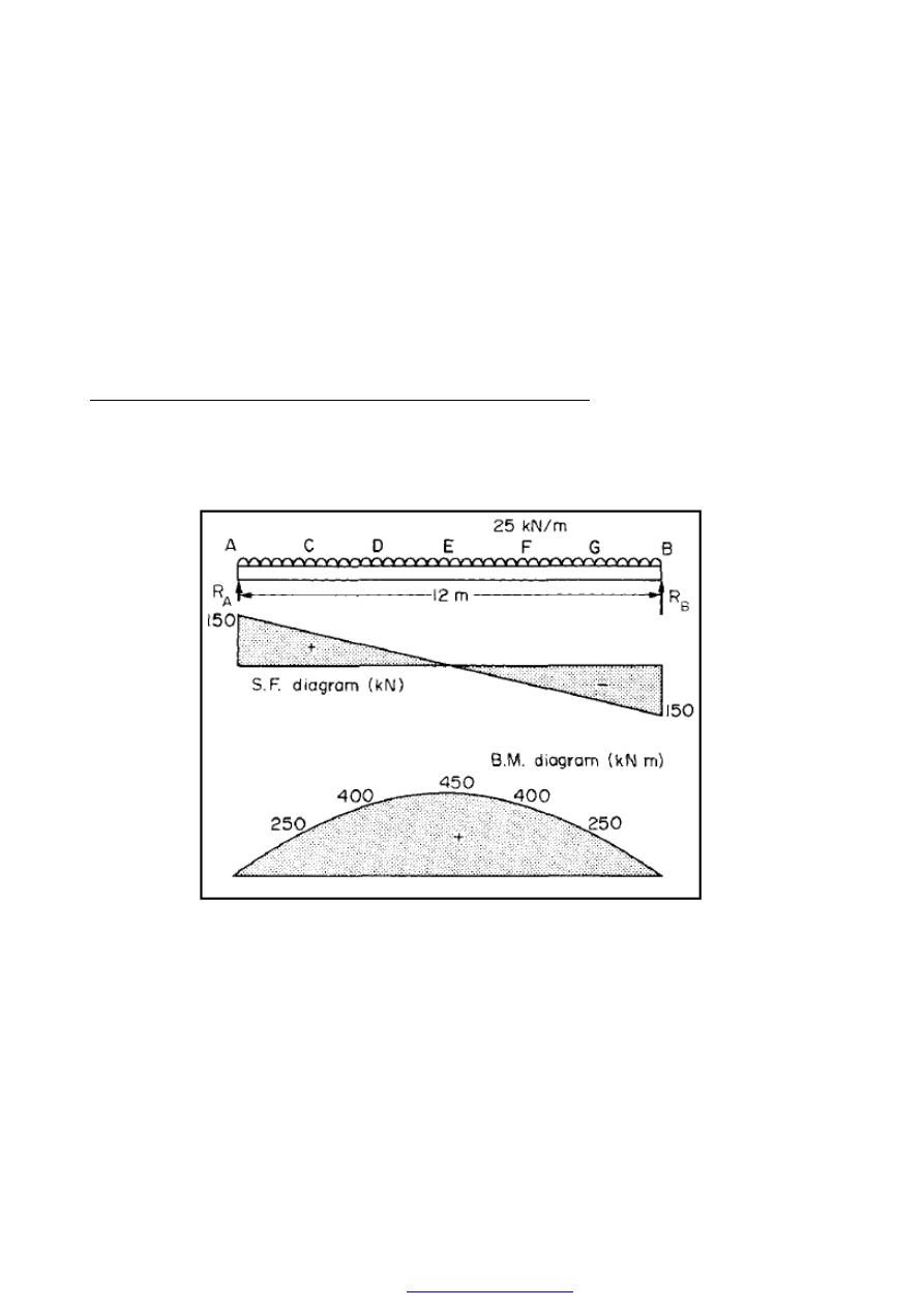
4. S.F. and B.M. diagrams for uniformly distributed loads
Consider now the simply supported beam shown in Figure (11) carrying a u.d.1. w = 25
kN/m across the complete span.
Figure (11)
Here again it is necessary to evaluate the reactions, but in this case the problem is
simplified by the symmetry of the beam. Each reaction will therefore take half the
applied load,
i.e.
PDF created with pdfFactory Pro trial version
44
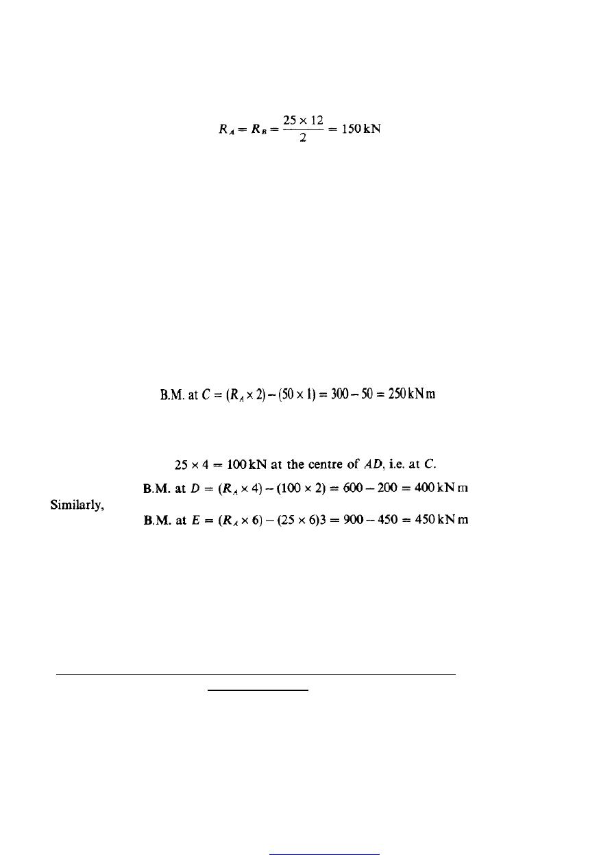
The S.F. at A, using the usual sign convention, is therefore + 150kN.
is, therefore, Consider now the beam divided into six equal parts 2 m long. The S.F. at
any other point C
150 - load downwards between A and C
= 150 - (25 x 2) = + 100 kN
The whole diagram may be constructed in this way, or much more quickly by noticing
that the S.F. at A is + 150 kN and that between A and B the S.F. decreases uniformly,
producing the required sloping straight line, shown in Fig. 3.7. Alternatively, the S.F. at
A is + 150 kN and between A and B this decreases gradually by the amount of the
applied load (By 25 x 12 = 300kN) to - 150kN at B. When evaluating B.M.’s it is
assumed that a u.d.1. can be replaced by a concentrated load of equal value acting at the
middle of its spread. When taking moments about C, therefore, the portion of the u.d.1.
between A and C has an effect equivalent to that of a concentrated load of
25 x 2 = 50 kN acting the centre of AC, i.e. 1 m from C.
Similarly, for moments at D the u.d.1. on AD can be replaced by a concentrated load of
The B.M. diagram will be symmetrical about the beam centre line; therefore the values of
B.M. at F and G will be the same as those at D and C respectively. The final diagram is
therefore as shown in Figure (11) and is parabolic.
Point (a) of the summary is clearly illustrated here, since the B.M. is a
maximum when the S.F. is zero. Again, the reason for this will be shown later.
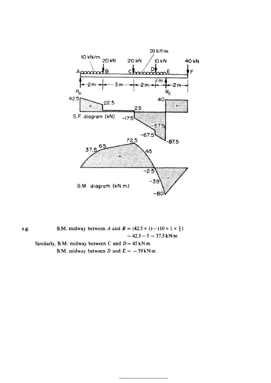
5. S.F. and B.M. diagrams for combined concentrated and uniformly
distributed loads
Consider the beam shown in Figure (12) loaded with a combination of concentrated loads
and u.d.1.s.
Taking moments about E
PDF created with pdfFactory Pro trial version
45
Working from the left-hand support it is now possible to construct the S.F. diagram, as
indicated previously, by following the direction arrows of the loads. In the case of the
u.d.l.’s the S.F. diagram will decrease gradually by the amount of the total load until the
end of the u.d.1. or the next concentrated load is reached. Where there is no u.d.1. the
S.F. diagram remains horizontal between load points. In order to plot the B.M. diagram
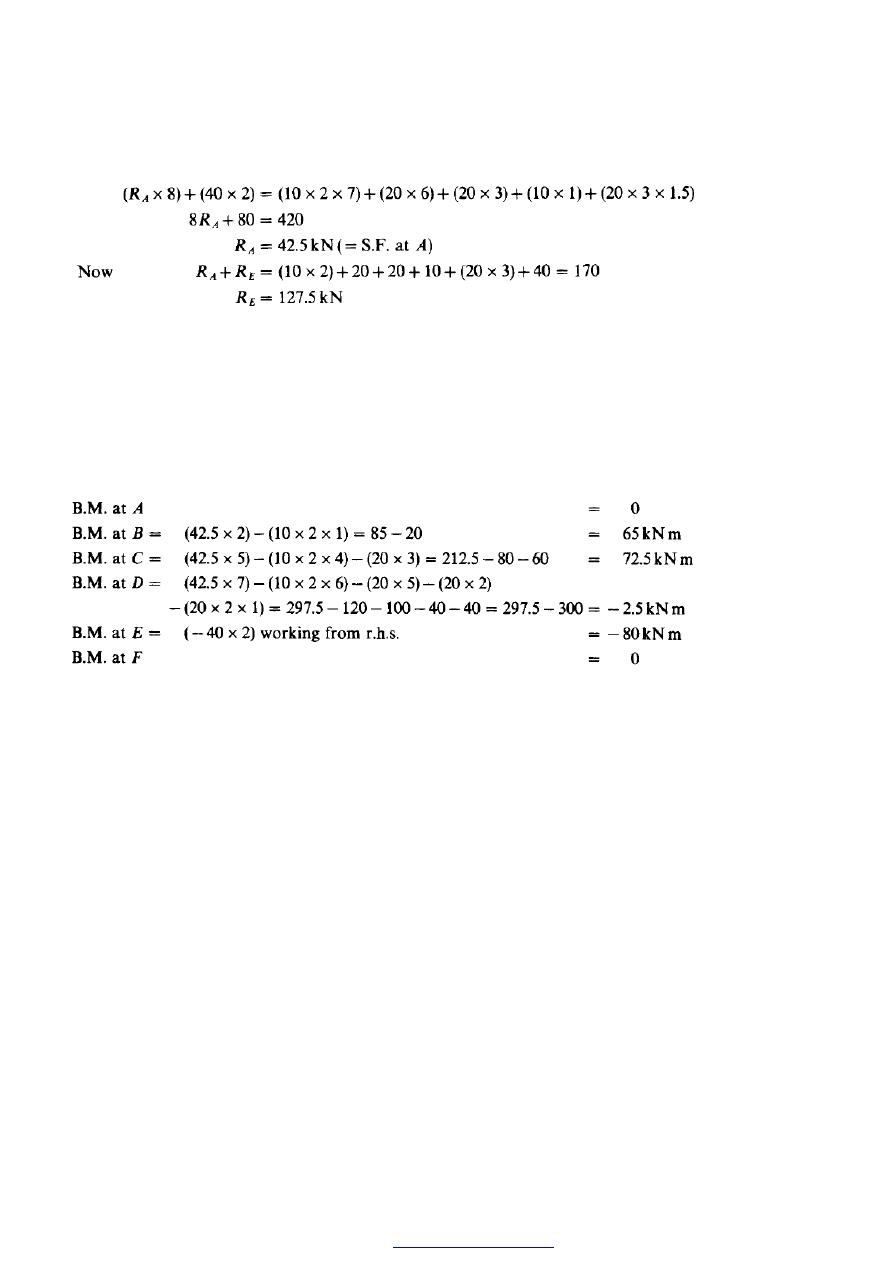
the following values must be determined:
PDF created with pdfFactory Pro trial version
46
Figure (12)
For complete accuracy one or two intermediate values should be obtained along each
u.d.l. portion of the beam,
The B.M. and S.F. diagrams are then as shown in Figure (12)
PDF created with pdfFactory Pro trial version
47
5. Points of contraflexure
A point of contraflexure is a point where the curvature of the beam changes sign. It is
sometimes referred to as a point of inflexion and will be shown later to occur at the point,
or points, on the beam where the B.M. is zero.
For the beam of Figure (9) therefore, it is evident from the B.M. diagram that this point
lies somewhere between C and D (B.M. at C is positive, B.M. at D is negative). If the
required point is a distance x from C then at that point
Since the last answer can be ignored (being outside the beam), the point of contraflexure
must be situated at 1.96 m to the right of C.
6. Relationship between shear force Q, bending moment M and
intensity of loading W (kN/m)
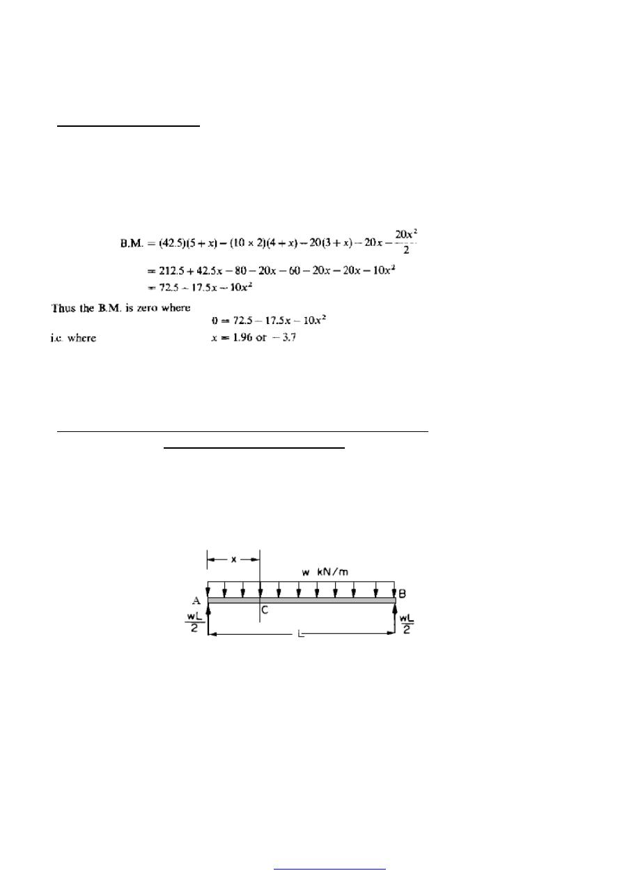
Consider the beam AB shown in Figure (10) carrying a uniform loading intensity
(uniformly distributed load) of W (kN/m). By symmetry, each reaction takes half the total
load, i.e., WL/2.
Figure (10)
PDF created with pdfFactory Pro trial version
48
Differentiating equation (1),
W
dx
dQ
−
=
.....(3)
These relationships are the basis of the rules stated in the summary, the proofs of which
are as follows:
(a) The maximum or minimum B.M. occurs where
0
=
dx
dM
But
Q
dx
dM
=
Thus where S.F. is zero B.M. is a maximum or minimum.
(b) The slope of the B.M. diagram =
Q
dx
dM
=
Thus where Q = 0 the slope of the B.M. diagram is zero, and the B.M. is therefore
constant.
(c) Also, since Q represents the slope of the B.M. diagram, it follows that where the S.F.
is positive the slope of the B.M. diagram is positive, and where the S.F. is negative the
slope of the B.M. diagram is also negative.
(d) The area of the S.F. diagram between any two points, from basic calculus, is
∫
dx
Q
But,
Q
dx
dM
=
or
∫
=
dx
Q
M
PDF created with pdfFactory Pro trial version
49
i.e. the B.M. change between any two points is the area of the S.F. diagram between these
points.
This often provides a very quick method of obtaining the B.M. diagram once the S.F.
diagram has been drawn.
(e) With the chosen sign convention, when the B.M. is positive the beam is sagging and
when it is negative the beam is hogging. Thus when the curvature of the beam changes
from sagging to hogging, as at x-x in Figure (11), or vice versa, the B.M.
changes sign, i.e. becomes instantaneously zero. This is termed a point of inflexion or
contra flexure. Thus a point of contra flexure occurs where the B.M. is zero.
Figure (11) Beam with point contraflexure at X-X
7. S.F. and B.M. diagrams for an applied couple or moment
In general there are two ways in which the couple or moment can be applied: (a) with
horizontal loads and (b) with vertical loads, and the method of solution is different for
each.
Type (a): couple or moment applied with horizontal loads
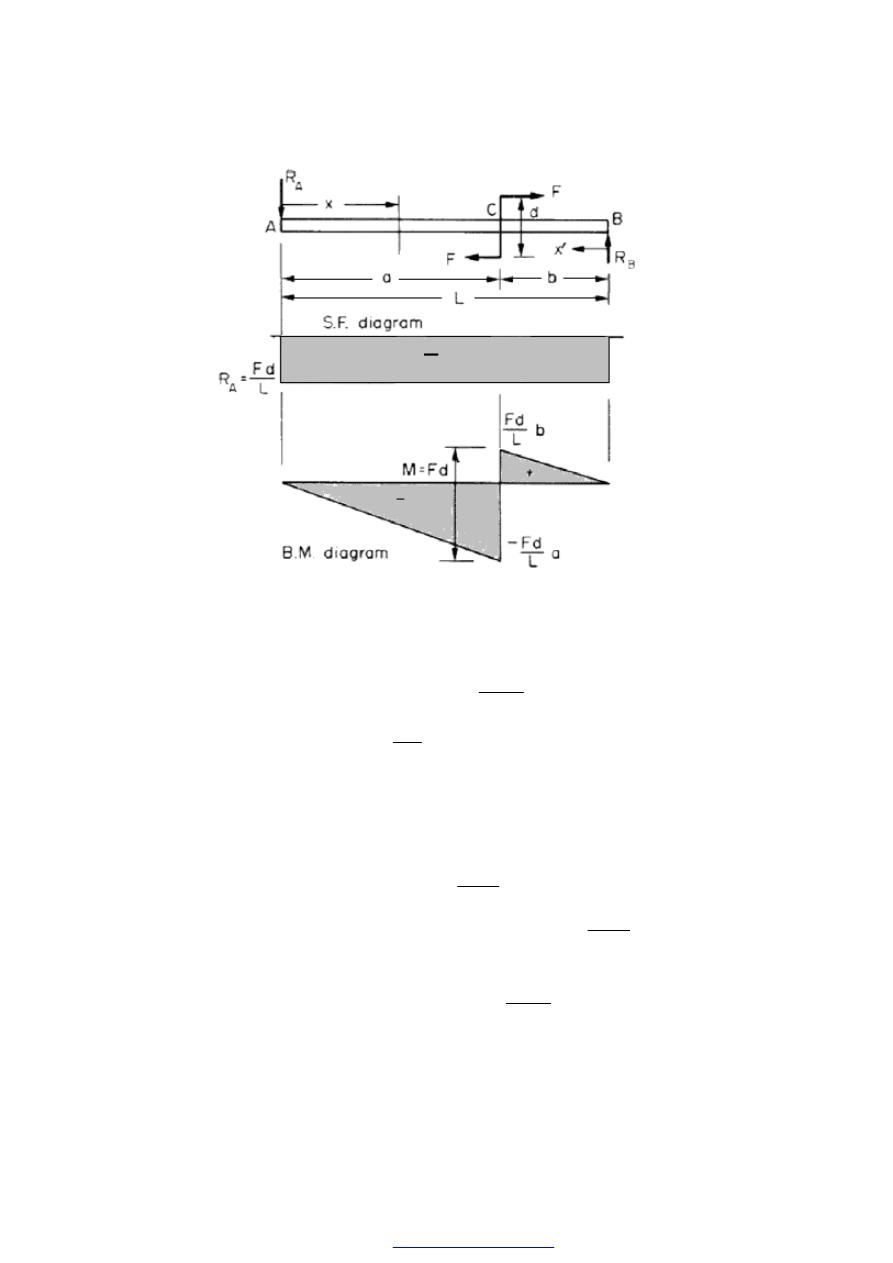
Consider the beam AB shown in Figure (12) to which a moment (F.d) is applied
by means of horizontal loads at a point C, distance a from A.
PDF created with pdfFactory Pro trial version
50
Figure (12)
Since this will tend to lift the beam at A, R
A
acts downwards.
Moments about B:
d
F
L
A
R
.
.
=
,
L
d
F
A
R
.
=
and for vertical equilibrium
L
d
F
A
R
B
R
.
=
=
The S.F. diagram can now
be drawn as the horizontal loads have no effect on the vertical
shear.
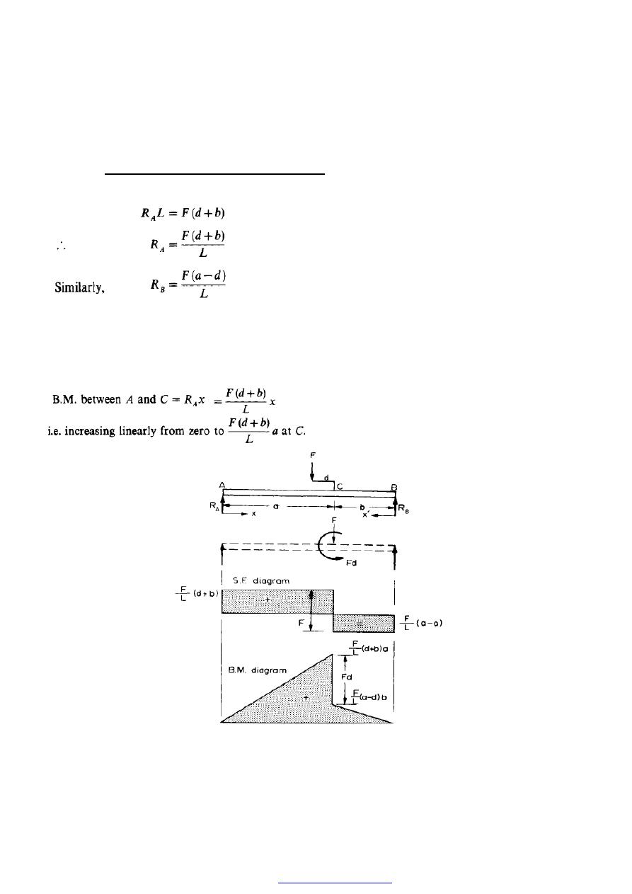
The B.M. at any section between A and C is
x
L
d
F
x
A
R
M
.
.
.
−
=
−
=
Thus the value of the B.M. increases linearly from zero at A to
a
L
d
F
.
.
−
at C
Similarly, the B.M. at any section between C and B is
x
L
d
F
x
B
R
d
F
x
A
R
M
.
.
.
.
.
−
=
=
+
−
=
PDF created with pdfFactory Pro trial version
51
i.e. the value of the B.M. again increases linearly from zero at B to - b at C. The B.M.
diagram is therefore as shown in Figure (12).
Type (b): moment applied with vertical loads
Consider the beam AB shown in Figure (13); taking moments about B:
The S.F. diagram can therefore be drawn as in Figure (13) and it will be observed that in
this case (F) does affect the diagram. For the B.M. diagram an equivalent system is used.
The offset load F is replaced by a
moment and a force acting at C, as shown in Figure
(13). Thus
Figure (13)
PDF created with pdfFactory Pro trial version
52
Examples
Example 1
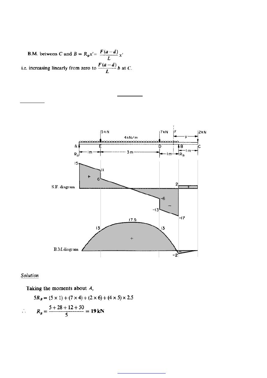
Draw the S.F. and B.M. diagrams for the beam loaded as shown in Figure
(14), and determine(a) the position and magnitude of the maximum B.M., and (b) the
position of any point of contraflexure.
Figure (14)
PDF created with pdfFactory Pro trial version
53
The S.F. diagram may now be constructed as shown in Figure (14) .
Calculation of bending moments
The maximum B.M. will be given by the point (or points) at which dM/dx (Le. the shear
force) is zero. By inspection of the S.F. diagram this occurs midway between D and E,
i.e. at1.5 m from E.
The B.M. diagram is therefore as shown in Figure (14) Alternatively, the B.M. at any
point between D and E at a distance of x from A will be given by
(b) Since the B.M. diagram only crosses the zero axis once there is only one point of
contraflexure, i.e. between B and D. Then, B.M. at distance y from C will be given by
The point of contraflexure occurs where B.M. = 0, i.e. where M
yy
= 0,
i.e. point of contraflexure occurs 0.12 m to the left of B.
PDF created with pdfFactory Pro trial version
54
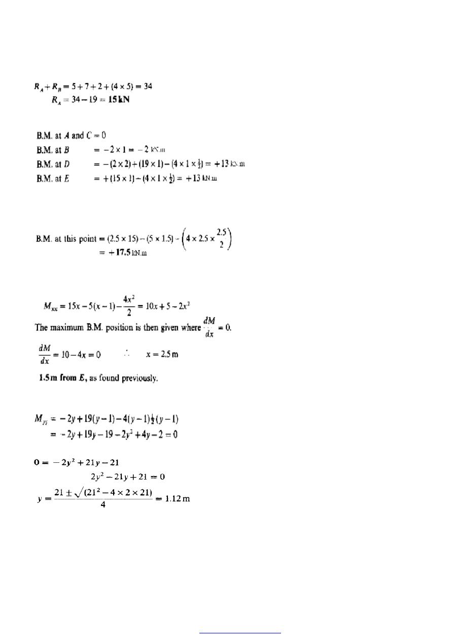
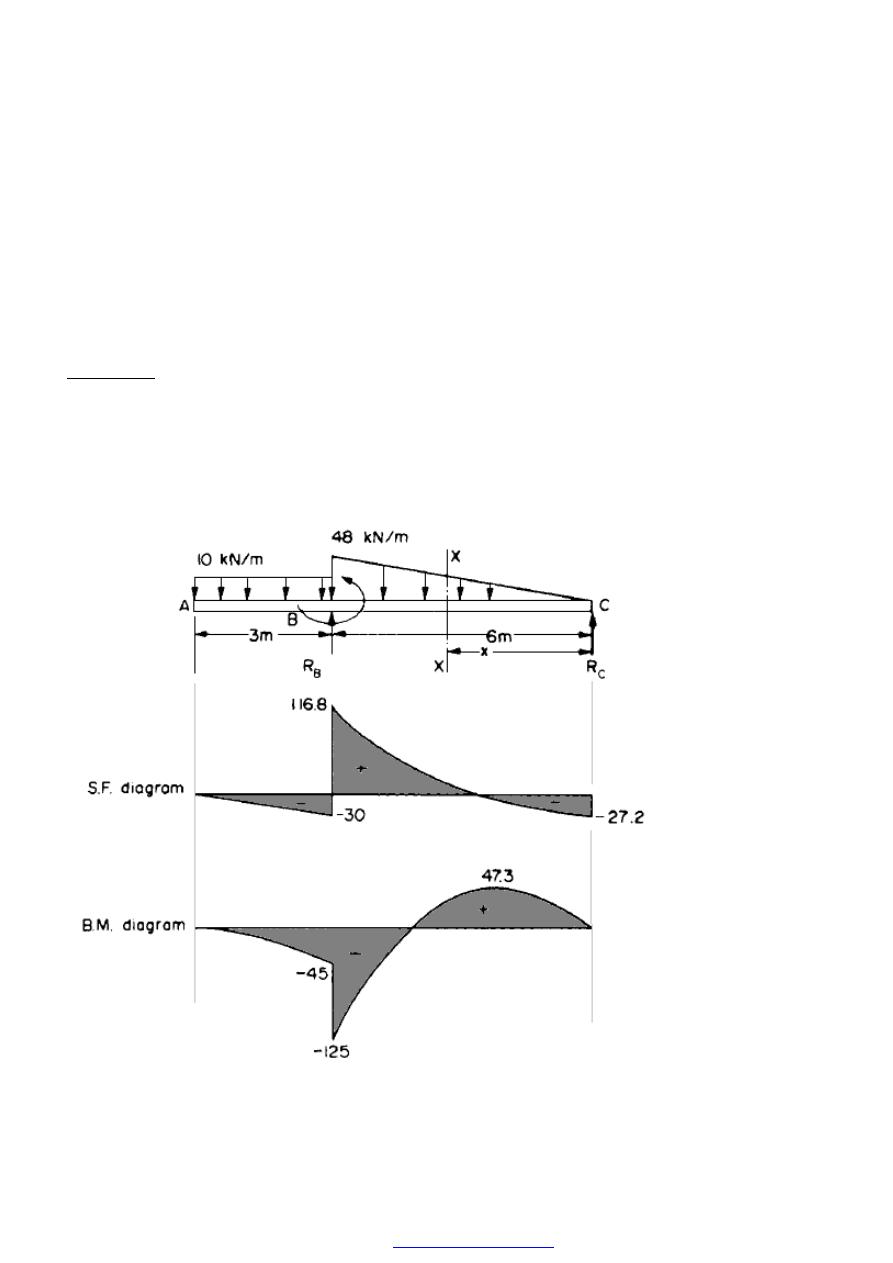
Example 2
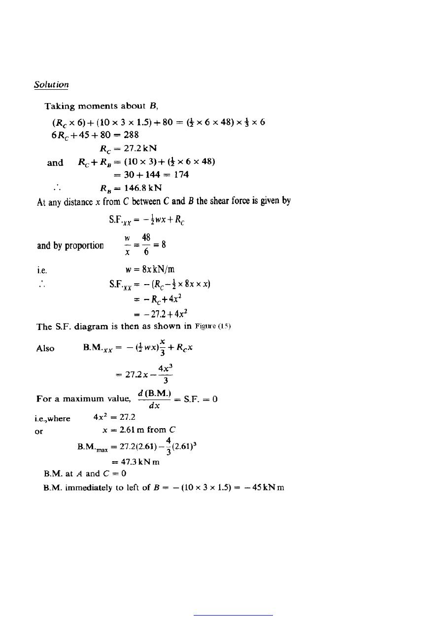
A beam ABC is 9 m long and supported at B and C, 6 m apart as shown in Figure (15).
The beam carries a triangular distribution of load over the portion BC together with an
applied counterclockwise couple of moment 80 kN m at B and a uniform distributed load
(u.d.1.) of 10 kN/m over AB, as shown. Draw the S.F. and B.M. diagrams for the beam.
Figure (15)
PDF created with pdfFactory Pro trial version
55
At the point of application of the applied moment there will be a sudden change in B.M. of 80 kN.
m. (There will be no such discontinuity in the S.F. diagram; the effect of the moment will merely
be reflected in the values calculated for the reactions.) The B.M. diagram is therefore as shown in
Figure (15).
PDF created with pdfFactory Pro trial version

56
Problems
1. A beam AB, 1.2 m long, is simply-supported at its ends A and B and carries two
concentrated loads, one of 10 kN at C, the other 15 kN at D. Point C is 0.4 m from A,
point D is 1 m from A. Draw the S.F. and B.M. diagrams for the beam inserting
principal values.
[9.17, - 0.83, -15.83 kN; 3.67, 3.17 kN.m]
2 . The beam of question (1) carries an additional load of 5 kN upwards at point E, 0.6 m
from A. Draw the S.F. and B.M. diagrams for the modified loading. What is the
maximum B.M.?
[6.67, -3.33, 1.67, -13.33 kN; 2.67, 2, 2.67 kN.m.]
3. A cantilever beam AB, 2.5 m long is rigidly built in at A and carries vertical
concentrated loads of 8 kN at B and 12 kN at C, 1 m from A. Draw S.F. and B.M.
diagrams for the beam inserting principal values.
[-8, -20 kN; -11.2, -31.2kN.m]
4. A beam AB, 5 m long, is simply-supported at the end B and at a point C, 1 m from A.
It carries vertical loads of 5 kN at A and 20kN at D, the centre of the span BC. Draw
S.F. and B.M. diagrams for the beam inserting principal values. [ - 5 , 11.25, -
8.75kN; - 5 , 17.5 kN.m]
5. A beam AB, 3 m long, is simply-supported at A and E. It carries a 16 kN concentrated
load at C, 1.2 m from A, and a u.d.1. of 5 kN/m over the remainder of the beam. Draw
the S.F. and B.M. diagrams and determine the value of the maximum B.M.
[12.3, -3.7, -12.7kN; 14.8 kN.m.]
6. A simply supported beam has a span of 4m and carries a uniformly distributed load of
60 kN/m together with a central concentrated load of 40 kN. Draw the S.F. and B.M.
diagrams for the beam and hence determine the maximum B.M. acting on the beam.
[S.F. 140, k20, -140 kN; B.M. 0, 160,0 kN.m]
7. A 2 m long cantilever is built-in at the right-hand end and carries a load of 40 kN at
the free end. In order to restrict the deflection of the cantilever within reasonable
limits an upward load of 10 kN is applied at mid-span. Construct the S.F. and B.M.
PDF created with pdfFactory Pro trial version

57
diagrams for the cantilever and hence determine the values of the reaction force and
moment at the support. [30 kN, 70 kN. m.]
8. A beam 4.2 m long overhangs each of two simple supports by 0.6 m. The beam carries
a uniformly distributed load of 30 kN/m between supports together with concentrated
loads of 20 kN and 30 kN at the two ends. Sketch the S.F. and B.M. diagrams for the
beam and hence determine the position of any points of contraflexure.
[S.F. -20, +43, -47, +30 kN; B.M. - 12, 18.75, - 18kN.m; 0.313 and 2.553 from
left hand support.]
9. A beam ABCDE, with A on the left, is 7 m long and is simply supported at Band E.
The lengths of the various portions are AB = 1.5 m, BC = 1.5 m, CD = 1
m and DE = 3 m. There is a uniformly distributed load of 15 kN/m between B and a
point 2 m to the right of B and concentrated loads of 20 kN act at A and D with one of
50 kN at C.
(a) Draw the S.F. diagrams and hence determine the position from A at which the S.F. is
zero.
(b) Determine the value of the B.M. at this point.
(c) Sketch the B.M. diagram approximately to scale, quoting the principal values.
[3.32 m; 69.8 kN,m; 0, -30, 69.1, 68.1, 0 kN.m]
10. A beam ABCDE is simply supported at A and D. It carries the following loading: a
distributed load of 30 kN/m between A and B a concentrated load of 20 kN at B; a
concentrated load of 20 kN at C; a concentrated load of 10 kN at E; a distributed
load of 60 kN/m between D and E. Span AB = 1.5 m, BC = CD = DE = 1 m.
Calculate the value of the reactions at A and D and hence draw the S.F. and B.M.
diagrams. What are the magnitude and position of the maximum B.M. on the beam?
[41.1, 113.9kN; 28.15kN.m; 1.37 m from A.]
PDF created with pdfFactory Pro trial version
58
T
T
O
O
R
R
S
S
I
I
O
O
N
N
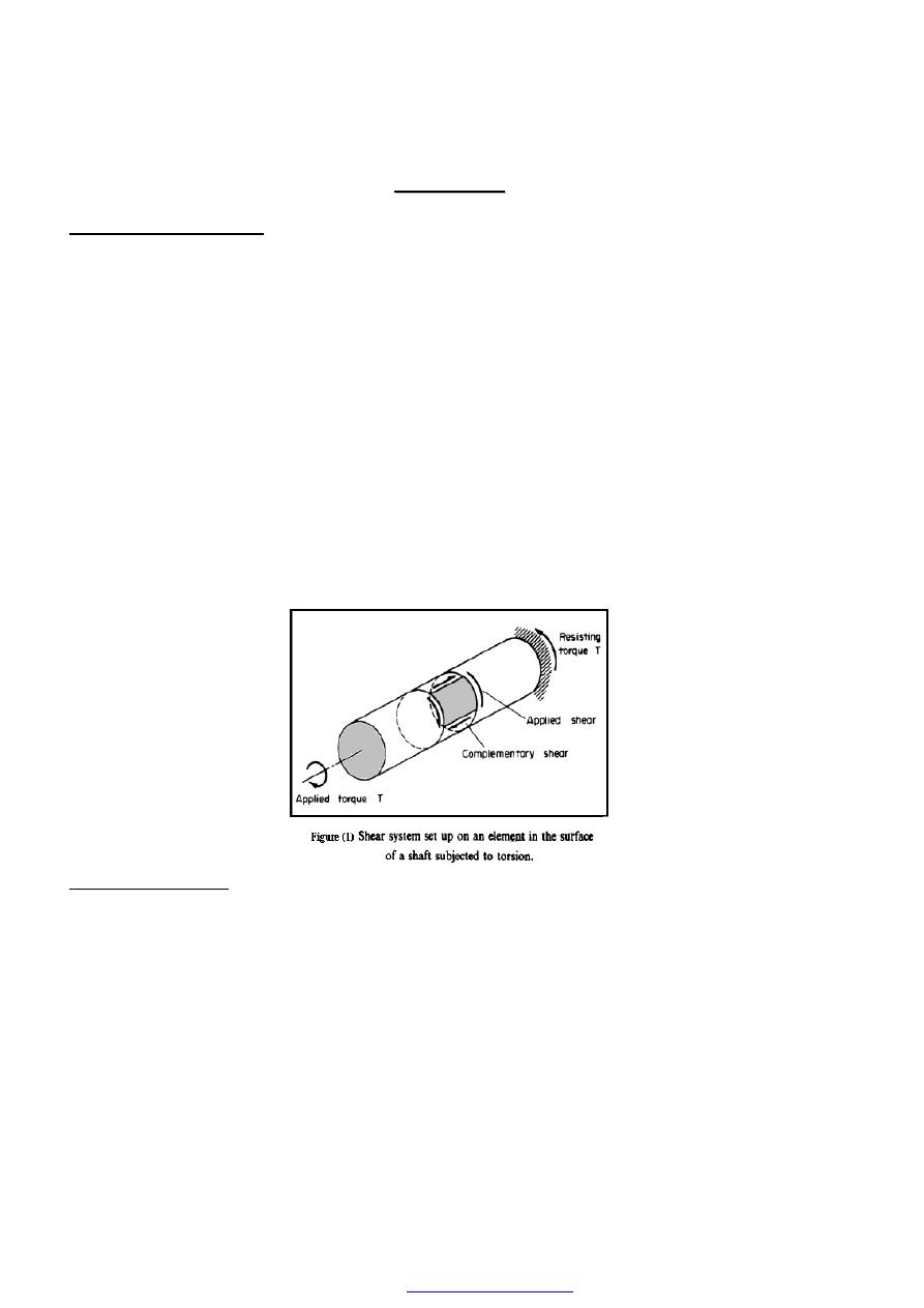
Simple torsion theory
When a uniform circular shaft is subjected to a torque it can be shown that every section
of the shaft is subjected to a state of pure shear Figure (1), the moment of resistance
developed by the shear stresses being everywhere equal to the magnitude, and opposite in
sense, to the applied torque. For the purposes of deriving a simple theory, to make the
following basic assumptions:
(1) The material is homogeneous, i.e. of uniform elastic properties throughout.
(2) The material is elastic, following Hooke's law with shear stress proportional to shear
strain.
(3) The stress does not exceed the elastic limit or limit of proportionality.
(4) Circular Sections remain circular.
(5) Cross-sections remain plane. (This is certainly not the case with the torsion of non
circular Sections.)
(6) Cross-sections rotate as if rigid, i.e. every diameter rotates through the same angle.
Practical tests carried out on circular shafts have shown that the theory developed below
on the basis of these assumptions shows excellent correlation with experimental results.
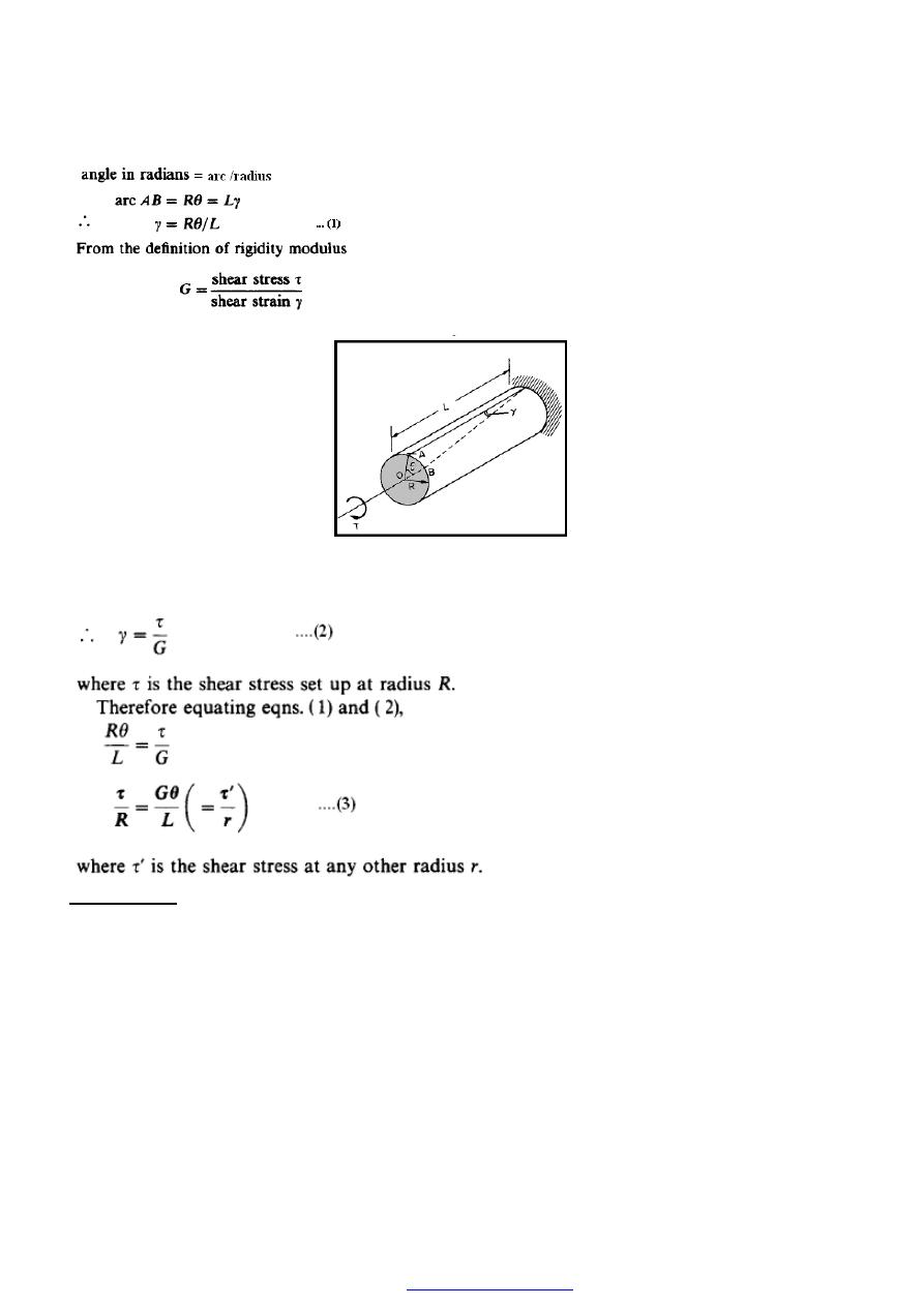
(a) Angle of twist
Consider now the solid circular shaft of radius (R) subjected to a torque (T) at one
end, the other end being fixed Figure (2). Under the action of this torque a radial
line at the free end of the shaft twists through an angle (
θ)
, point A moves to B, and AB
subtends an angle (
γ)
at the fixed end. This is then the angle of distortion of the shaft, i.e.
the shear strain.
PDF created with pdfFactory Pro trial version
59
Figure (2)
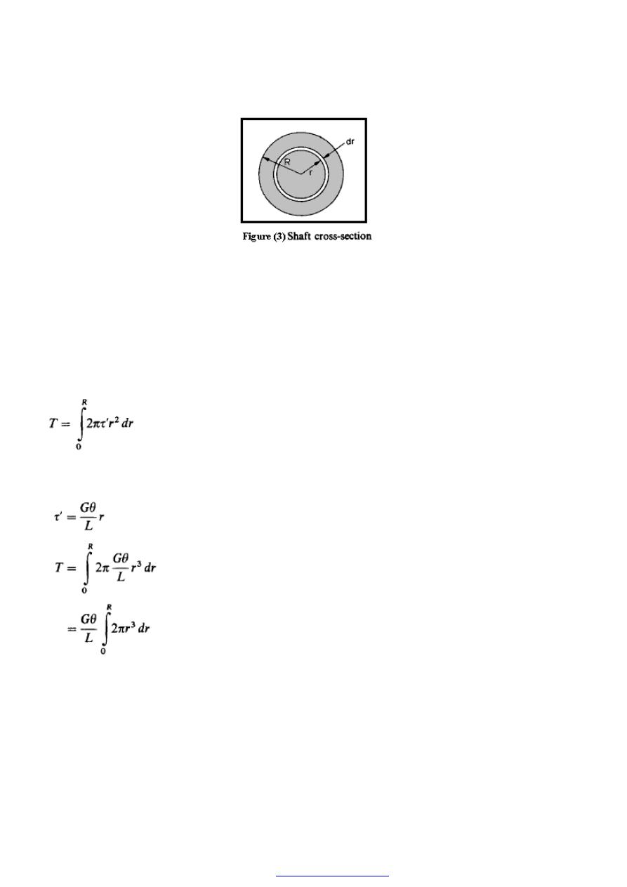
(b) Stresses
Let the cross-section of the shaft be considered as divided into elements of radius r
and thickness (dr) as shown in Figure (3) each subjected to a shear stress (
τ
').
PDF created with pdfFactory Pro trial version
60
The force set up on each element,
= stress x area=
τ
' x 2.
π.r dr (approximately)
This force will produce a moment about the centre axis of the shaft, providing a
contribution to the torque
=
(τ
' x 2.
π.r dr
)
.r=
τ
' x 2.
π.r
2
dr
The total torque on the section (T) will then be the sum of all such contributions across
the section,
Now the shear stress (
τ') will vary with the radius rand must therefore be replaced in
terms of r before the integral is evaluated. From eqnuation (3)
The integral
∫
R
dr
r
0
3
.
.
.
2
π
is called the polar second moment of area (J), and may be
evaluated as a
standard form for solid and hollow shafts .
PDF created with pdfFactory Pro trial version
61
Combining eqns. (3) and (4) produces the so-called simple theory of torsion:
Polar second moment of area
As
stated above the polar second moment
of
area J
is
defined as
For a solid shaft,
For
a
hollow shaft
of internal radius r,
For thin-walled hollow shafts the values of (D) and (d) may be nearly equal, and in such
cases there can be considerable errors in using the above equation involving the
difference of two large quantities of similar value. It is therefore convenient to obtain an
alternative form of expression for the polar moment of area.
Now
PDF created with pdfFactory Pro trial version
62
Where; A = 2
π
r dr is the area of each small element of Figure (3).
If a thin hollow cylinder is therefore considered as just one of these small elements with
its wall thickness t = dr, then
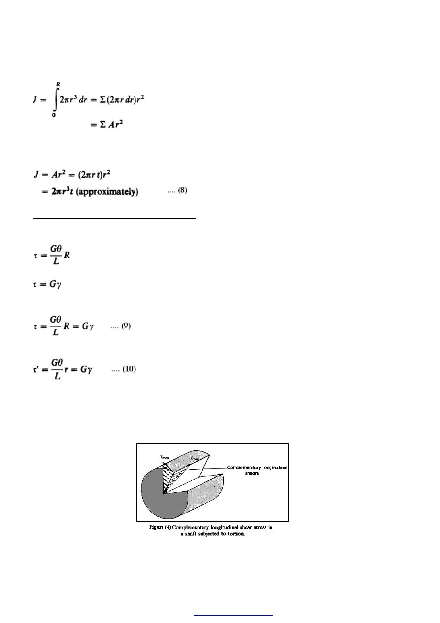
Shear stress and shear strain in shafts
The shear stresses which are developed in a shaft subjected to pure torsion are indicated
in Figure (1),their values being given by the simple torsion theory as
Now from the definition of the shear or rigidity modulus (G),
It therefore follows that the two equations may be combined to relate the shear stress and
strain in the shaft to the angle of twist per unit length, thus
or, in terms of some internal radius r,
These equations indicate that the shear stress and shear strain vary linearly with radius
and have their maximum value at the outside radius Figure (4) .
PDF created with pdfFactory Pro trial version
63
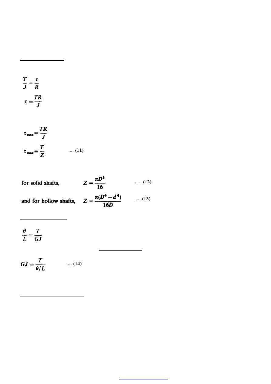
Section modulus
It is sometimes convenient to re-write part of the torsion theory formula to obtain the
maximum shear stress in shafts as follows:
With (R) the outside radius of the shaft the above equation yields the greatest value
possible for T, Figure (4).
Where; z = J/R is termed the polar section modulus. It will be seen from the preceding
section that:
Torsional rigidity
The angle of twist per unit length of shafts is given by the torsion theory as
The quantity (GJ) is termed the torsional rigidity of the shaft and is thus given by
i.e. the torsional rigidity is the torque divided by the angle of twist (in radians) per unit
length
.
Torsion of hollow shafts
It has been shown above that the maximum shear stress in a solid shaft is developed in
the outer surface, values at other radii decreasing linearly to zero at the centre. In
applications where weight reduction is of prime importance as in the aerospace industry,
for instance, it is often found advisable to use hollow shafts.
PDF created with pdfFactory Pro trial version
64
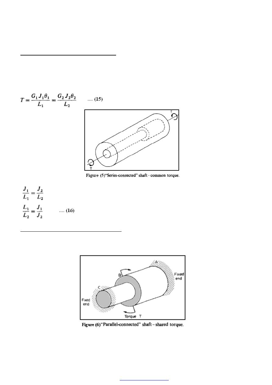
Composite shafts - series connection
If two or more shafts of different material, diameter or basic form are connected
together in such a way that each carries the same torque, then the shafts are said to be
connected in series and the composite shaft so produced is therefore termed series-
connected Figure (5) .
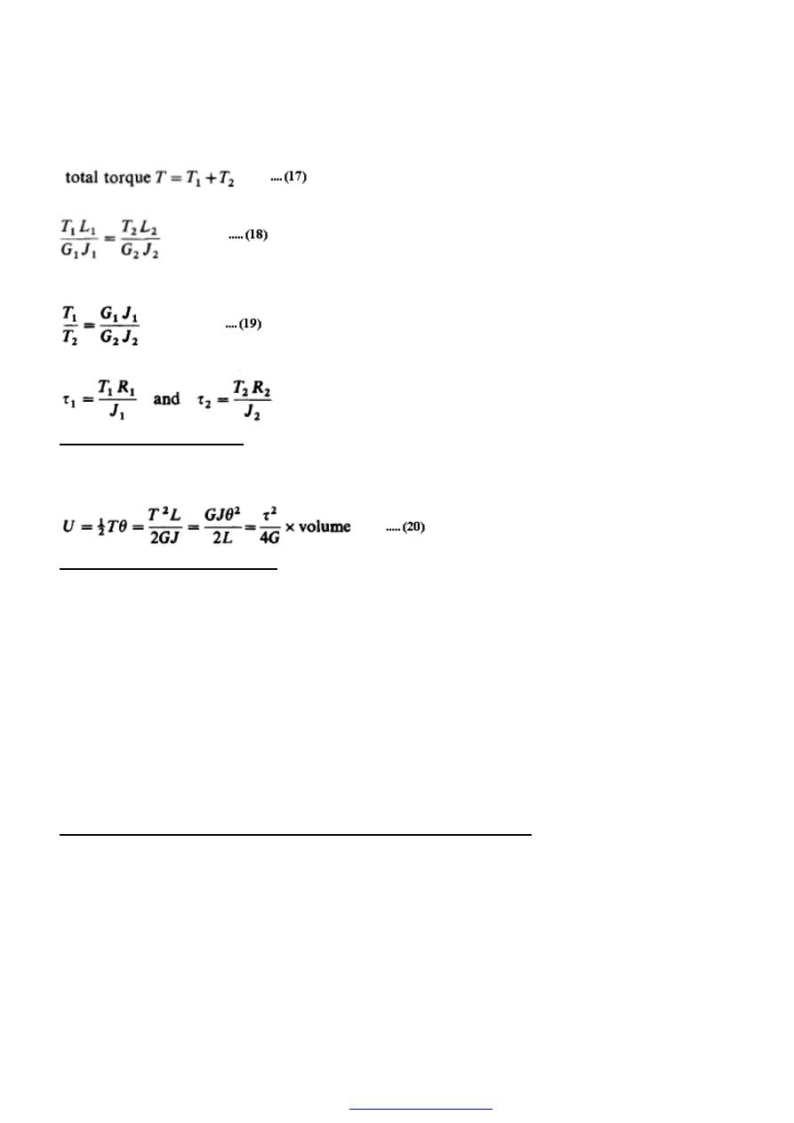
Composite shafts - parallel connection
If two or more materials are rigidly fixed together such that the applied torque is shared
between them then the composite shaft so formed is said to be connected in parallel
Figure (6).
PDF created with pdfFactory Pro trial version
65
For parallel connection,
In this case the angles of twist of each portion are equal and
i.e. for equal lengths (as is normally the case for parallel shafts)
The maximum stresses in each part can then be found from
Strain energy in torsion
The strain energy stored in a solid circular bar or shaft subjected to a torque (T) is given
by the alternative expressions.
Power transmitted by shafts
If a shaft carries a torque T Newton metres and rotates at o rad/s it will do work at the
rate of;
T.
ω
Nm/s (or joule/s).
Now the rate at which a system works is defined as its power, the basic unit of power
being the
Watt (1 Watt = 1 N.m/s).
Thus, the power transmitted by the shaft:
=
T.
ω
Watts.
Since the Watt is a very small unit of power in engineering terms use is normally made of
SI. multiples, i.e. kilowatts (kW) or megawatts (MW).
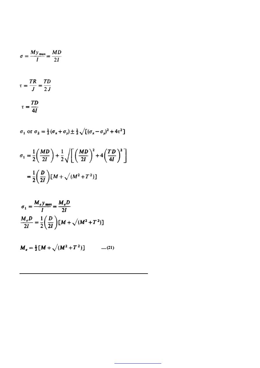
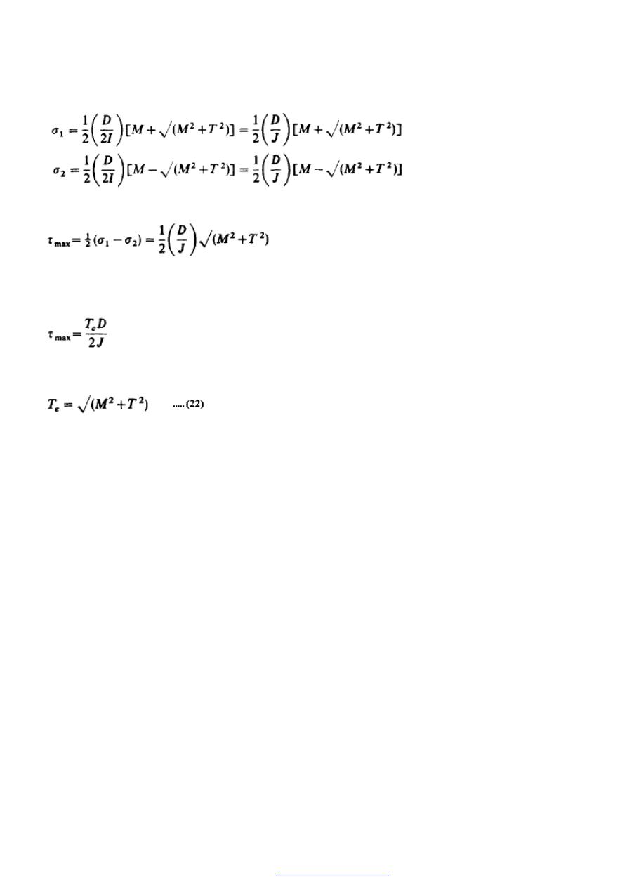
Combined bending and torsion - equivalent bending moment
For shafts subjected to the simultaneous application of a bending moment (M) and torque
(T) the principal stresses set up in the shaft can be shown to be equal to those produced
by an equivalent bending moment, of a certain value (M
e
) acting alone.
From the simple bending theory the maximum direct stresses set up at the outside surface
of the shaft owing to the bending moment (M) are given by
PDF created with pdfFactory Pro trial version
66
Similarly, from the torsion theory, the maximum shear stress in the surface of the shaft is
given by
But for a circular shaft J = 2I,
The principal stresses for this system can now be obtained by applying the formula
derived in
and, with
σ
y
= 0, the maximum principal stress (
σ
1
) is given by
Now if (M
e
) is the bending moment which, acting alone, will produce the same
maximum stress, then
i.e. the equivalent bending moment is given by
and it will produce the same maximum direct stress as the combined bending and torsion
effects.
Combined bending and torsion - equivalent torque
Again considering shafts subjected to the simultaneous application of a bending moment
(M) and a torque (T) the maximum shear stress set up in the shaft may be determined
by the application of an equivalent torque of value (T
e
) acting alone. From the preceding
section the principal stresses in the shaft are given by
PDF created with pdfFactory Pro trial version
67
Now the maximum shear stress is given by equation (12)
But, from the torsion theory, the equivalent torque T
e ,
will set up a maximum shear
stress of
Thus if these maximum shear stresses are to be equal,
PDF created with pdfFactory Pro trial version
68
Examples
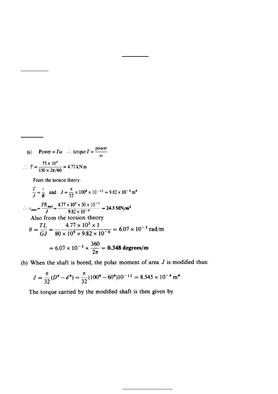
Example 1
(a) A solid shaft, 100 mm diameter, transmits 75 kW at 150 rev/min. Determine the value
of the maximum shear stress set up in the shaft and the angle of twist per metre of the
shaft length if G = 80 GN/m
2
.
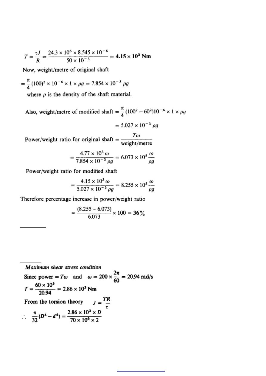
(b) If the shaft were now bored in order to reduce weight to produce a tube of 100 mm
outside diameter and 60mm inside diameter, what torque could be carried if the same
maximum shear stress is not to be exceeded? What is the percentage increase in
power/weight ratio effected by this modification?
Solution
PDF created with pdfFactory Pro trial version
69
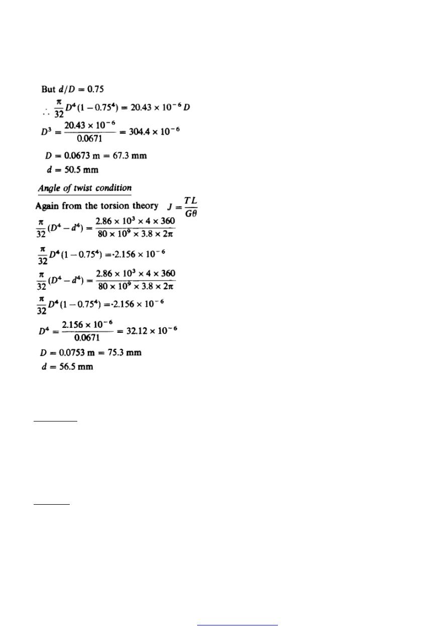
Example 2
Determine the dimensions of a hollow shaft with a diameter ratio of 3:4 which is to
transmit 60 kW at 200 rev/min. The maximum shear stress in the shaft is limited to
70 MN/m
2
and the angle of twist to 3.8
o
in a length of 4 m. For the shaft material G =
80 GN/m
2
.
Solution
PDF created with pdfFactory Pro trial version
70
Thus the dimensions required for the shaft to satisfy both conditions are outer diameter
75.3mm; inner diameter 56.5 mm.
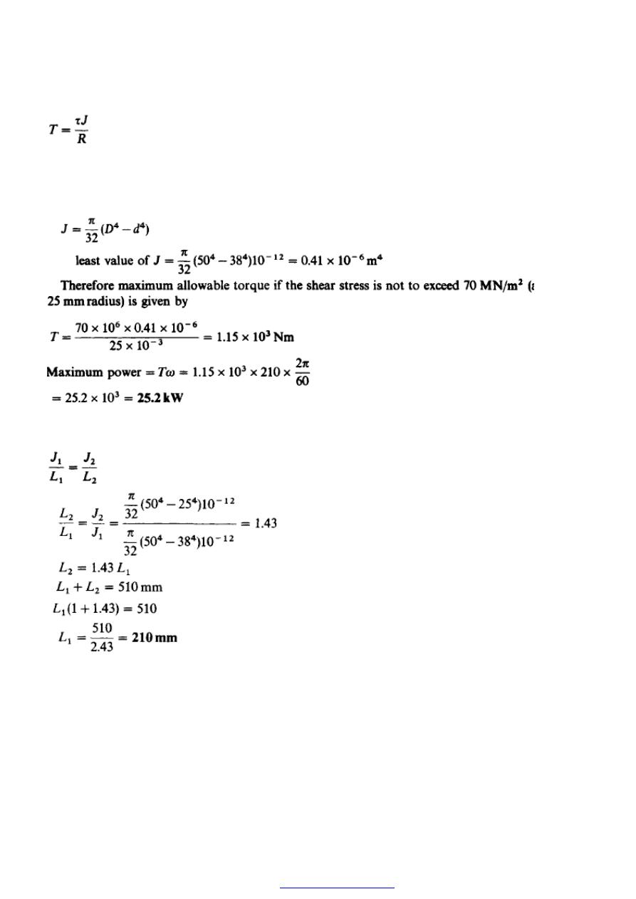
Example 3
(a) A steel transmission shaft is 510 mm long and 50 mm external diameter. For part of
its length it is bored to a diameter of 25 mm and for the rest to 38 mm diameter. Find the
maximum power that may be transmitted at a speed of 210 rev/min if the shear
stress is not to exceed 70 MN/m
2
.
(b) If the angle of twist in the length of 25 mm bore is equal to that in the length of 38
mm bore, find the length bored to the latter diameter.
Solution
(a) This is, in effect, a question on shafts in series since each part is subjected to the same
torque. From the torsion theory ;
PDF created with pdfFactory Pro trial version
71
and as the maximum stress and the radius at which it occurs (the outside radius) are the
same for both shafts the torque allowable for a known value of shear stress is dependent
only on the value of (J). This will be least where the internal diameter is greatest since
(
b)
Let suffix 1 refer to the 38 mm diameter bore portion and suffix 2 to the other part. Now
for shafts in series, equation (16) applies
,
PDF created with pdfFactory Pro trial version

72
PROBLEMS
1 - A solid steel shaft (A) of 50 mm diameter rotates at 250 rev/min. Find the greatest power that can be
transmitted for a limiting shearing stress of 60 MN/m
2
in the steel.
It is proposed to replace (A) by a hollow shaft ( B), of the Same external diameter but with
a limiting shearing stress of 75 MN/m
2
. Determine the internal diameter of (B) to transmit the same
power at the same speed.
A
A
n
n
s
s
.
.
[
[
3
3
8
8
.
.
6
6
k
k
W
W
,
,
3
3
3
3
.
.
4
4
m
m
m
m
]
]
2 - Calculate the dimensions of a hollow steel shaft which is required to transmit 750 kW at a speed of
400 rev/min if the maximum torque exceeds the mean by 20 % and the greatest intensity of shear
stress is limited to75 MN/m
2
. The internal diameter of the shaft is to be 80 % of the external
diameter. (The mean torque is that derived from the horsepower equation.)
A
A
n
n
s
s
.
.
[
[
1
1
3
3
5
5
.
.
2
2
m
m
m
m
,
,
1
1
0
0
8
8
.
.
2
2
m
m
m
m
.
.
]
]
3 - A steel shaft 3 m long is transmitting 1 MW at 240 rev/min. The working conditions to be satisfied
by the
shaft are:
(a) that the shaft must not twist more than 0.02 radian on a length of 10 diameters;
(b) that the working stress must not exceed 60 MN/m
2
.
If the modulus of rigidity of steel is 80 GN/m
2
what is
(i) the diameter of the shaft required
(ii) the actual working stress;
(iii) the angle of twist of the 3 m length?
A
A
n
n
s
s
.
.
[
[
l
l
5
5
0
0
m
m
m
m
;
;
6
6
0
0
M
M
N
N
/
/
m
m
2
2
;
;
0
0
.
.
0
0
3
3
0
0
r
r
a
a
d
d
.
.
]
]
4 - A hollow shaft has to transmit 6MW at 150 rev/min. The maximum allowable stress is not to exceed
60 MN/m
2
and the angle of twist 0.3
o
per metre length of shafting. If the outside diameter of the
shaft is 300 mm find the minimum thickness of the hollow shaft to satisfy the above conditions. G =
80 GN/m
2
.
A
A
n
n
s
s
.
.
[
[
6
6
1
1
.
.
5
5
m
m
m
m
.
.
]
]
5 - A flanged coupling having six bolts placed at a pitch circle diameter of 180 mm connects two lengths
of solid steel shafting of the same diameter. The shaft is required to transmit 80 kW at 240 rev/min.
Assuming the allowable intensities of shearing stresses in the shaft and bolts are 75 MN/m
2
and 55
MN/m
2
respectively, and the maximum torque is 1.4 times the mean torque, calculate:
(a) the diameter of the shaft;
(b) the diameter of the bolts.
A
A
n
n
s
s
.
.
[
[
6
6
7
7
.
.
2
2
m
m
m
m
,
,
1
1
3
3
.
.
8
8
m
m
m
m
.
.
]
]
6 - A hollow low carbon steel shaft is subjected to a torque of 0.25 MN. m. If the ratio of internal to
external diameter is 1 to 3 and the shear stress due to torque has to be limited to 70 MN/m
2
determine the required diameters and the angle of twist in degrees per metre length of shaft.
G = 80GN/m
2
.
A
A
n
n
s
s
.
.
[
[
2
2
6
6
4
4
m
m
m
m
,
,
8
8
8
8
m
m
m
m
;
;
0
0
.
.
3
3
8
8
o
o
]
]
PDF created with pdfFactory Pro trial version

73
CRYSTALLINE STRUCTURE OF METALS
The arrangement of atoms in a material determines the behavior and properties of that
material. Most of the materials used in the construction of a nuclear reactor facility are
metals. In this chapter, we will discuss the various types of bonding that occurs in
material selected for use in a reactor facility.
1- Atomic Bonding
There are three common states, these three states are solid, liquid, and gas. The
atomic or molecular interactions that occur within a substance determine its state. In this
chapter, we will deal primarily with solids because solids are of the most concern in
engineering applications of materials. Liquids and gases will be mentioned for
comparative purposes only. Solid matter is held together by forces originating between
neighboring atoms or molecules. These forces arise because of differences in the electron
clouds of atoms. In other words, the valence electrons, or those in the outer shell, of
atoms determine their attraction for their neighbors. When physical attraction between
molecules or atoms of a material is great, the material is held tightly together. Molecules
in solids are bound tightly together. When the attractions are weaker, the substance may
be in a liquid form and free to flow. Gases exhibit virtually no attractive forces between
atoms or molecules, and their particles are free to move independently of each other. The
types of bonds in a material are determined by the manner in which forces hold matter
together. Figure (1) illustrates several types of bonds and their characteristics
are listed below.
a. Ionic bond - In this type of bond, one or more electrons are wholly transferred from an
atom of one element to the atom of the other, and the elements are held together by the
force of attraction due to the opposite polarity of the charge.
b. Covalent bond - A bond formed by shared electrons. Electrons are shared when an
atom needs electrons to complete its outer shell and can share those electrons with its
neighbor. The electrons are then part of both atoms and both shells are filled.
c. Metallic bond - In this type of bond, the atoms do not share or exchange electrons to
bond together. Instead, many electrons (roughly one for each atom) are more or less
free to move throughout the metal, so that each electron can interact with many of the
fixed atoms.
PDF created with pdfFactory Pro trial version
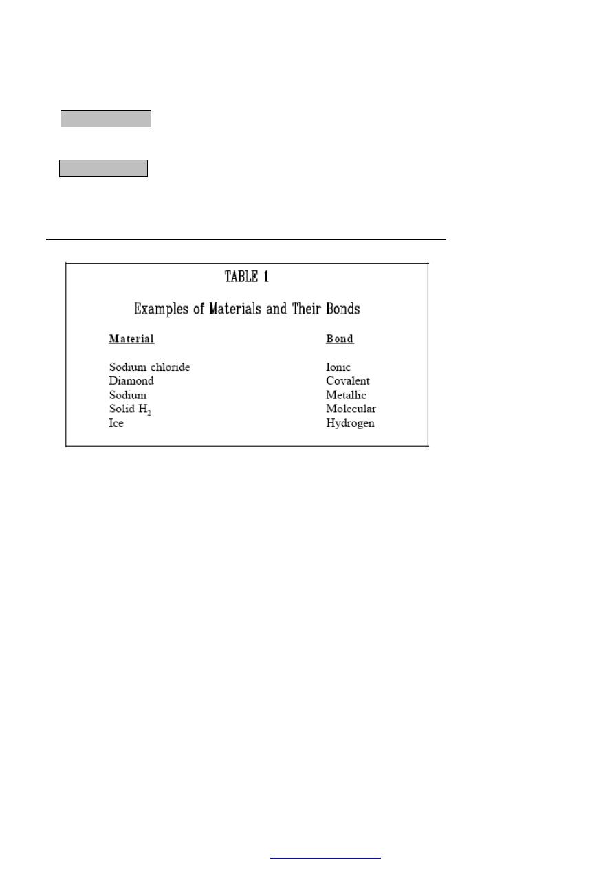
74
d. Molecular bond - When the electrons of neutral atoms spend more time in one region
of their orbit, a temporary weak charge will exist. The molecule will weakly attract
other molecules. This is sometimes called the van der Waals or molecular bonds.
e. Hydrogen bond - This bond is similar to the molecular bond and occurs due to the ease
with which hydrogen atoms are willing to give up an electron to atoms of oxygen,
fluorine, or nitrogen.
Some examples of materials and their bonds are identified in Table (1).
The type of bond not only determines how well a material is held together, but also
determines what microscopic properties the material possesses. Properties such as the
ability to conduct heat or electrical current are determined by the freedom of movement
of electrons. This is dependent on the type of bonding present. Knowledge of the
microscopic structure of a material allows us to predict how that material will behave
under certain conditions. Conversely, a material may be synthetically fabricated with
a given microscopic structure to yield properties desirable for certain engineering
applications.
PDF created with pdfFactory Pro trial version
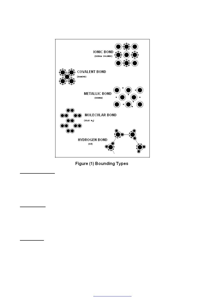
75
2- Microstructures
Solids have greater inter atomic attractions than liquids and gases. However, there are
wide variations in the properties of solid materials used for engineering purposes. The
properties of materials depend on their inter atomic bonds. These same bonds also dictate
the space between the configuration of atoms in solids. All solids may be classified as
either amorphous or crystalline.
3- Amorphous
Amorphous materials have no regular arrangement of their molecules. Materials like
glass and paraffin are considered amorphous. Amorphous materials have the properties of
solids. They have definite shape and volume and diffuse slowly. These materials also
lack sharply defined melting points. In many respects, they resemble liquids that flow
very slowly at room temperature.
4- Crystalline
In a crystalline structure, the atoms are arranged in a three-dimensional array called a
lattice. The lattice has a regular repeating configuration in all directions. A group of
PDF created with pdfFactory Pro trial version

76
particles from one part of a crystal has exactly the same geometric relationship as a group
from any other part of the same crystal.
COMMON LATTICE TYPES
All metals used in a reactor have crystalline structures. Crystalline microstructures are
arranged in three-dimensional arrays called lattices.
1- Crystal structure
In metals, and in many other solids, the atoms are arranged in regular arrays called
crystals. A crystal structure consists of atoms arranged in a pattern that repeats
periodically in a three-dimensional geometric lattice. The forces of chemical bonding
causes this repetition. It is this repeated pattern which control properties like strength,
ductility, density (described in Module 2, Properties of Metals), conductivity (property of
conducting or transmitting heat, electricity, etc.), and shape.
In general, the three most common basic crystal patterns associated with metals are: (I)
the body-centered cubic, (II) the face-centered cubic, and (III) the hexagonal close-
packed. Figure (2) shows these three patterns.
(I) Body-centered cubic structure
In a body-centered cubic (BCC) arrangement of atoms, the unit cell consists of eight
atoms at the corners of a cube and one atom at the body center of the cube.
(II) Face-centered cubic structure
In a face-centered cubic (FCC) arrangement of atoms, the unit cell consists of eight
atoms at the corners of a cube and one atom at the center of each of the faces of the cube.
(III) Hexagonal close-packed structure
In a hexagonal close-packed (HCP) arrangement of atoms, the unit cell consists of
three layers of atoms. The top and bottom layers contain six atoms at the corners of a
hexagon and one atom at the center of each hexagon. The middle layer contains three
atoms nestled between the atoms of the top and bottom layers, hence, the name close-
packed.
PDF created with pdfFactory Pro trial version
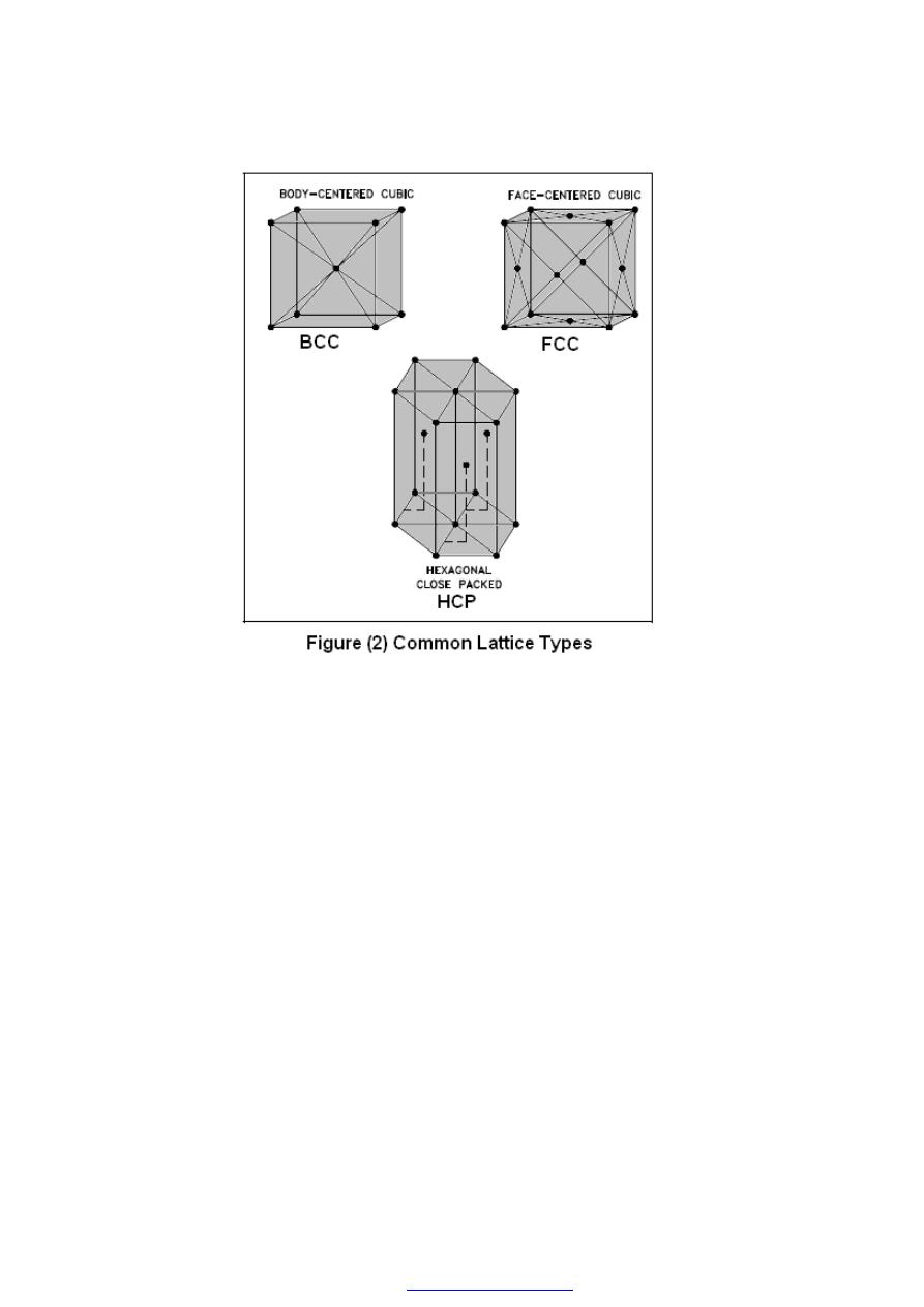
77
Most diagrams of the structural cells for the BCC and FCC forms of iron are drawn as
though they are of the same size, as shown in Figure ( 2) , but they are not. I n th e BCC
arrangement, the structural cell, which uses only nine atoms, is much smaller.
Metals such as
α
-iron (Fe) (ferrite), chromium (Cr), vanadium (V), molybdenum (Mo),
and tungsten (W) possess BCC structures. These BCC metals have two properties in
common, high strength and low ductility (which permits permanent deformation). FCC
metals such as
γ
-iron(Fe) (austenite), aluminum (Al), copper (Cu), lead (Pb), silver (Ag),
gold (Au), nickel (Ni), platinum (Pt), and thorium (Th) are, in general, of lower strength
and higher ductility than BCC metals. HCP structures are found in beryllium (Be),
magnesium (Mg), zinc (Zn), cadmium (Cd), cobalt (Co), thallium (Tl), and zirconium
(Zr). The important information in this chapter is summarized below.
PDF created with pdfFactory Pro trial version

78
GRAIN STRUCTURE AND BOUNDARY
Metals contain grains and crystal structures. The individual needs a microscope to see
the grains and crystal structures. Grains and grain boundaries help determine the
properties of a material.
1- Grain Structure and Boundary
If you were to take a small section of a common metal and examine it under a
microscope, you would see a structure similar to that shown in Figure 3(a). Each of the
light areas is called a grain, or crystal, which is the region of space occupied by a
continuous crystal lattice. The dark lines surrounding the grains are grain boundaries. The
grain structure refers to the arrangement of the grains in a metal, with a grain having a
particular crystal structure. The grain boundary refers to the outside area of a grain that
separates it from the other grains. The grain boundary is a region of misfit between the
grains and is usually one to three atom diameters wide. The grain boundaries separate
variously-oriented crystal regions(polycrystalline) in which the crystal structures are
identical. Figure 3(b) represents four grains of different orientation and the grain
boundaries that arise at the interfaces between the grains. A very important feature of a
metal is the average size of the grain. The size of the grain determines the properties of
the metal. For example, smaller grain size increases tensile strength and tends to increase
ductility. A larger grain size is preferred for improved high-temperature creep properties.
Creep is the permanent deformation that increases with time under constant load or
stress. Creep becomes progressively easier with increasing temperature. Stress and strain
are covered in Module 2, Properties of Metals, and creep is covered in Module 5,
Plant Materials.
Another important property of the grains is their orientation. Figure 4(a)
represents a random Figure (3) Grains and Boundaries (a) Microscopic (b)
Atomic arrangement of the grains such that no one direction within the grains is aligned
with the external boundaries of the metal sample. This random orientation can be
obtained by cross rolling the material. If such a sample were rolled sufficiently in one
direction, it might develop a grain-oriented structure in the rolling direction as shown in
Figure 4(b). This is called preferred orientation. In many cases, preferred orientation is
very desirable, but in other instances, it can be most harmful. For example, preferred
orientation in uranium fuel elements can result in catastrophic changes in dimensions
during use in a nuclear reactor.
PDF created with pdfFactory Pro trial version
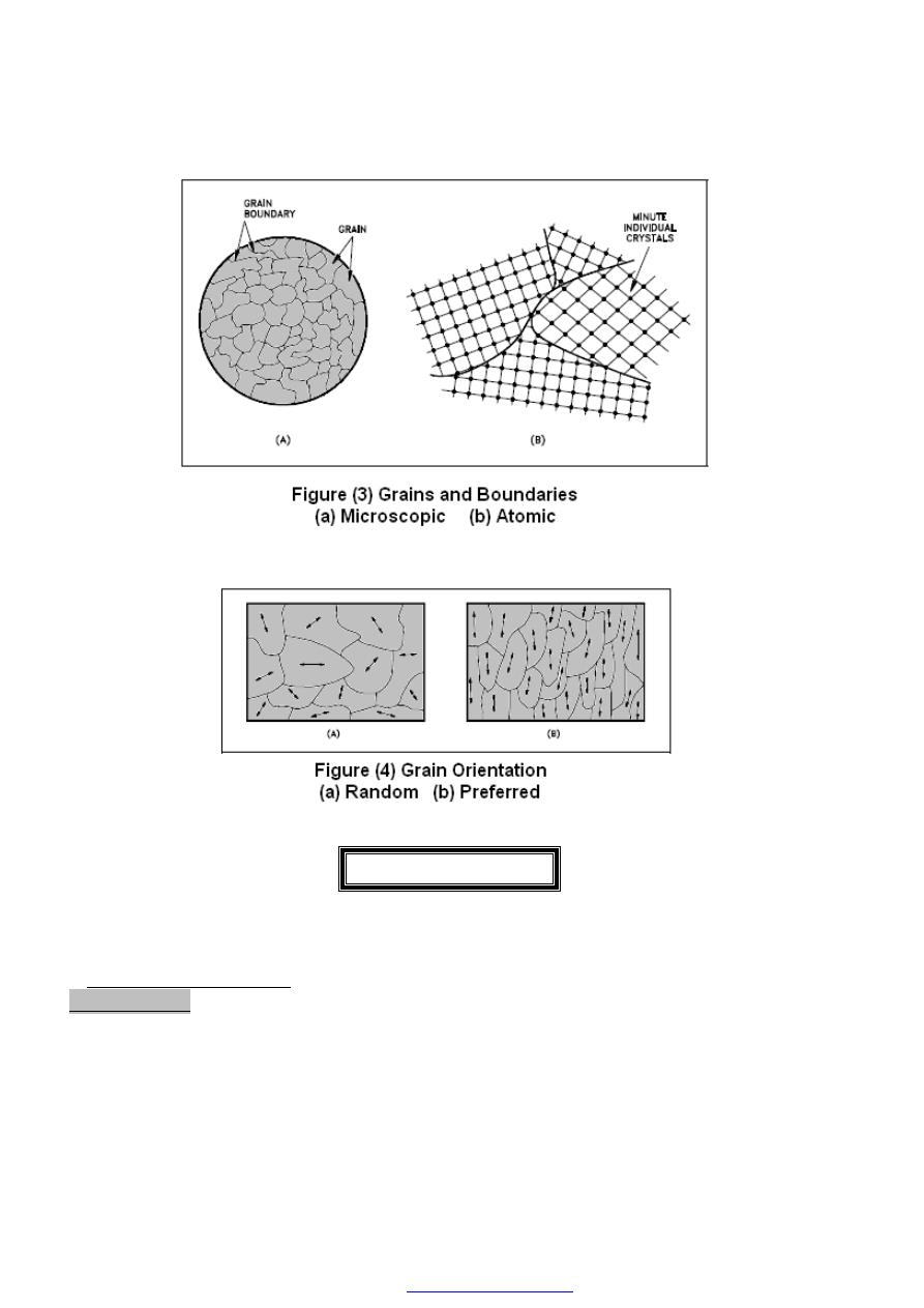
79
POLYMORPHISM
Metals are capable of existing in more than one form at a time. This chapter will discuss
this property of metals.
1- Polymorphism Phases
Polymorphism is the property Figure 5 Cooling Curve for Unalloyed Uranium or ability
of a metal to exist in two or more crystalline forms
depending upon temperature and composition. Most metals and metal alloys exhibit this
property. Uranium is a good example of a metal that exhibits polymorphism. Uranium
metal can exist in three different crystalline structures. Each structure exists at a specific
phase, as illustrated in Figure 5.
PDF created with pdfFactory Pro trial version
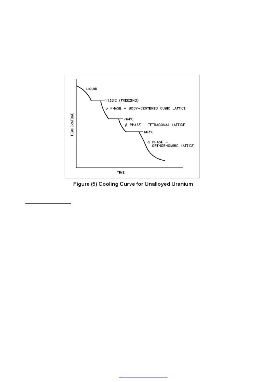
80
1. The alpha phase, from room temperature to 663
°
C
2. The beta phase, from 663
°
C to 764
°
C
3. The gamma phase, from 764
°
C to its melting point of 1133
°
C
2- Alpha (
α) Phase
The alpha (
α
) phase is stable at room temperature and has a crystal system
characterized by three unequal axes at right angles.
In the alpha phase, the properties of the lattice are different in the X, Y, and Z axes.
This is because of the regular recurring state of the atoms is different. Because of this
condition, when heated the phase expands in the X and Z directions and shrinks in the Y
direction. Figure 6 shows what happens to the dimensions (Å = angstrom, one hundred-
millionth of a centimeter) of a unit cell of alpha uranium upon being heated. As shown,
heating and cooling of alpha phase uranium can lead to drastic dimensional changes and
gross distortions of the metal. Thus, pure uranium is not used as a fuel, but only in alloys
or compounds. Figure 6 Change in Alpha Uranium Upon Heating From 0 to 300
°
C The
beta (
β
) phase of uranium occurs at elevated temperatures. This phase has a tetragonal
(having four angles and four sides) lattice structure and is quite complex.
PDF created with pdfFactory Pro trial version
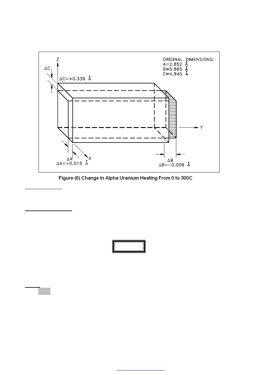
81
3- Beta
(
β)
Phase
The beta (
β
) phase of uranium occurs at elevated temperatures. This phase has a
tetragonal (having four angles and four sides) lattice structure and is quite complex.
hase
P
)
γ
amma (
G
-
4
The gamma (
γ
) phase of uranium is formed at temperatures above those required for
beta phase stability. In the gamma phase, the lattice structure is BCC and expands equally
in all directions when heated.
ALLOYS
Most of the materials used in structural engineering or component fabrication are
metals. Alloying is a common practice because metallic bonds allow joining of different
types of metals.
1- Alloy
An alloy is a mixture of two or more materials, at least one of which is a metal.
Alloys can have a microstructure consisting of solid solutions, where secondary atoms
are introduced as substitutionals or interstitials (discussed further in the next chapter and
Module 5, Plant Materials) in a crystal lattice. An alloy might also be a crystal with a
metallic compound at each lattice point. In addition, alloys may be composed of
PDF created with pdfFactory Pro trial version

82
secondary crystals imbedded in a primary polycrystalline matrix. This type of alloy is
called a composite (although the term "composite" does not necessarily imply that the
component materials are metals). Module2, Properties of Metals, discusses how different
elements change the physical properties of a metal.
2- Common Characteristics of Alloys
Alloys are usually stronger than pure metals, although they generally offer reduced
electrical and thermal conductivity. Strength is the most important criterion by which
many structural materials are judged. Therefore, alloys are used for engineering
construction. Steel, probably the most common structural metal, is a good example of an
alloy. It is an alloy of iron and carbon, with other elements to give it certain desirable
properties. As mentioned in the previous chapter, it is sometimes possible for a material
to be composed of several solid phases. The strengths of these materials are enhanced by
allowing a solid structure to become a form composed of two interspersed phases. When
the material in question is an alloy, it is possible to quench (discussed in more detail in
Module 2, Properties of Metals) the metal from a molten state to form the interspersed
phases. The type and rate of quenching determines the final solid structure and, therefore,
its properties.
PDF created with pdfFactory Pro trial version
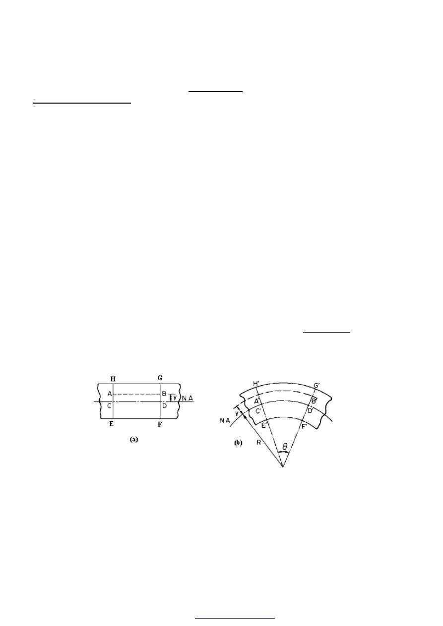
83
BENDING
Simple bending theory
If a piece of rubber, most conveniently of rectangular cross-section, is bent between
one’s fingers it is readily apparent that one surface of the rubber is stretched, i.e. put into
tension, and the opposite surface is compressed. In order for this to be achieved it is
necessary to make certain simplifying assumptions. The assumptions are as follows:
(1) The beam is initially straight and unstressed.
(2) The material of the beam is perfectly homogeneous and isotropic, i.e. of the same
density and elastic properties throughout.
(3) The elastic limit is nowhere exceeded.
(4) Young's modulus for the material is the same in tension and compression.
(5) Plane cross-sections remain plane before and after bending.
(6) Every cross-section of the beam is symmetrical about the plane of bending, i.e. about
an
(7) There is no resultant force perpendicular to any cross-section.
If we now consider a beam initially unstressed and subjected to a constant (B.M.)
along its length, i.e. pure bending, as would be obtained by applying equal couples at
each end, it will bend to a radius (R ) as shown in Figure (1b). As a result of this bending
the top fibres of the beam will be subjected to tension and the bottom to compression. It
is reasonable to suppose, therefore, that somewhere between the two there are points at
which the stress is zero. The locus of all such points is termed the neutral axis (N.A). The
radius of curvature R is then measured to this axis. For symmetrical sections the N.A. is
the axis of symmetry, but whatever the section the N.A. will always pass through the
centre of area or centroid.
.
Figure (1) Beam subjected to pure bending
(a) before, and (b) after, the moment
Consider now two cross-sections of a beam, HE and GF, originally parallel
Figure (1a) When the beam is bent Figure (1b). it is assumed that these sections remain
PDF created with pdfFactory Pro trial version
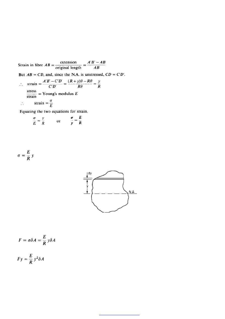
84
plane; i.e. H' E' and G'F', the final positions of the sections, are still straight lines. They
will then subtend some angle (
θ). Consider now some fibre AB in the material, distance y
from the N.A. When the beam is bent this will stretch to A'B'.
……..(1)
Consider now a cross-section of the beam Figure (2) From equation (1) the stress on a
fibre at distance (y) from the N.A. is
Figure (2) Beam cross-section.
If the strip is of area
δA the force on the strip is
This has a moment about the N.A. of
The total moment for the whole cross-section is therefore
PDF created with pdfFactory Pro trial version
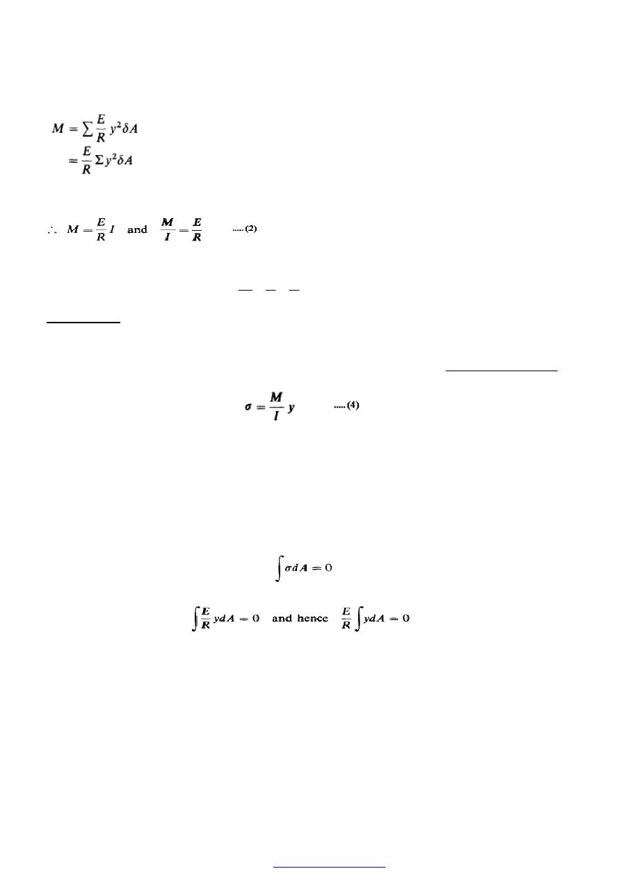
85
since (E) and (R) are assumed constant.
The term
∑
A
y
δ
.
2
is called the second moment
of
area of the cross-section and given the symbol (I).
Combining eqns. (1) and (2) we have the bending theory equation
)
3
......(
R
E
y
I
M
=
=
σ
Neutral axis
In bending, one surface of the beam is subjected to tension and the opposite surface to
compression there must be a region within the beam cross-section at which the stress
changes sign, i.e. where the stress is zero, and this is termed the neutral axis (N.A).
Further, equation (3) may be re-written in the form
which shows that at any section the stress is directly proportional to y, the distance from
the N.A., i.e. (s) varies linearly with (y), the maximum stress values occurring in the
outside surface of the beam where (y) is a maximum.
The force on the small element of area is (s.dA) acting perpendicular to the cross-
section, i.e. parallel to the beam axis. The total force parallel to the beam axis is
therefore
∫
dA
.
σ
. The tensile force on one side of the N.A. must exactly balance the
compressive force on the other side
Substituting from equation (1)
Typical stress distributions in bending are shown in Figure (4). In order to obtain the
maximum resistance to bending it is advisable therefore to use sections which have large
areas as far away from the N.A. as possible. For this reason beams with I- or T-sections
find considerable favour in present engineering applications, such as girders, where
bending plays a large part. Such beams have large moments of area about one axis and,
provided that it is ensured that bending takes place about this axis, they will have a high
resistance to bending stresses.
PDF created with pdfFactory Pro trial version
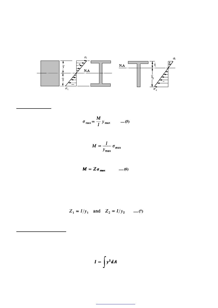
86
Figure (4) Typical bending stress distributions
.
Section modulus
From equation (4) the maximum stress obtained in any cross-section is given by
For any given allowable stress the maximum moment which can be accepted by a
particular shape of cross-section is therefore
For ready comparison of the strength of various beam cross-sections this is sometimes
written in the form
where Z(= I/y
max.
) is termed the section modulus. The higher the value of Z for
a particular cross-section the higher the B.M. which it can withstand for a given
maximum stress. This is particularly important in the case of unsymmetrical sections
such as T-sections where the values of (y
max
) wi1l also be different on each side of the
N.A. Figure (4) and here two values of section modulus are often quoted,
each being then used with the appropriate value of allowable stress.
Second moment of area
Consider the rectangular beam cross-section shown in Figure (5) and an element of
area (dA), thickness (dy), breadth (B) and distance (y) from the N.A. which by symmetry
passes through the centre of the section. The second moment of area (I) has been defined
earlier as
PDF created with pdfFactory Pro trial version

87
Thus for the rectangular section the second moment of area about the N.A., i.e. an axis
through the centre, is given by
Similarly, the second moment of area of the rectangular section about an axis through the
lower edge of the section would be found using the same procedure but with integral
limits of 0 to D.
These standard forms prove very convenient in the determination of (I
N.A.
) values for
built-up sections which can be conveniently divided into rectangles. For symmetrical
sections as, for instance, the I-section shown in Figure (6)
PDF created with pdfFactory Pro trial version
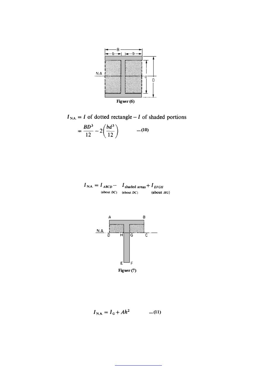
88
It will be found that any symmetrical section can be divided into convenient rectangles
with the N.A. running through each of their centroids and the above procedure can then
be employed to effect a rapid solution. For unsymmetrical sections such as the T-section
of Figure (7) it is more convenient to divide the section into rectangles with their edges in
the N.A., when the second type of standard form may be applied.
(each of these quantities may be written in the form BD
3
/3).
As an alternative procedure it is possible to determine the second moment of area of each
rectangle about an axis through its own centroid (I
G
= 8D
3
/12) and to “shift” this value to
the equivalent value about the N.A. by means of the parallel axis theorem.
PDF created with pdfFactory Pro trial version
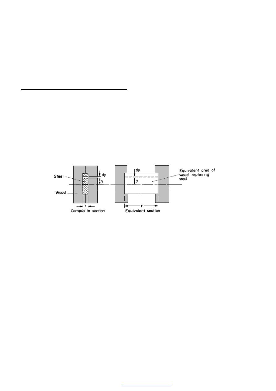
89
Where;(A) is the area of the rectangle and (h) the distance of its centroid (G) from the
N.A. Whilst this is perhaps not so quick or convenient for sections built-up from
rectangles.
Bending of composite or flitched beams
(a) A composite beam is one which is constructed from a combination of materials. If
such a beam is formed by rigidly bolting together two timber joists and reinforcing steel
plate, a then it is termed a flitched beam.
Since the bending theory only holds good when a constant value of Young’s
modulus applies across a section it cannot be used directly to solve composite-beam
problems where two different materials, and therefore different values of (E), are
present. The method of solution in such a case is to replace one of the materials by an
equivalent section of the other
.
Figure (8) Bending of composite or flitched beams: original beam cross-section and
equivalent of uniform material (wood) properties.
Consider, therefore, the beam shown in Figure (8) in which a steel plate is held centrally
in an appropriate recess between two blocks of wood. Here it is convenient to replace the
steel by an equivalent area of wood, retaining the same bending strength, i.e. the moment
at any section must be the same in the equivalent section as in the original so that the
force at any given (dy) in the equivalent beam must be equal to that at the strip it
replaces.
PDF created with pdfFactory Pro trial version
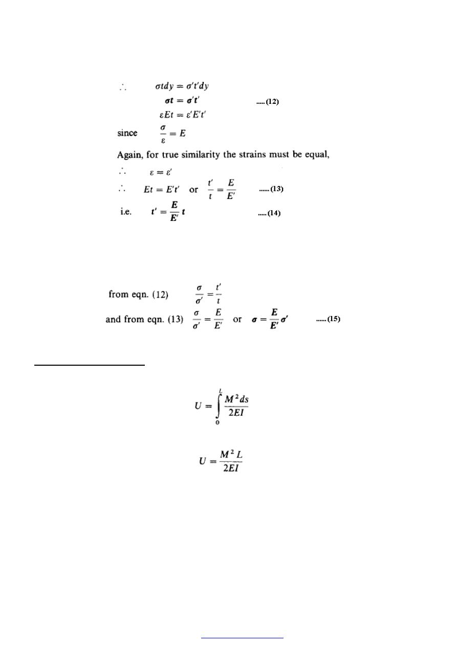
90
Thus to replace the steel strip by an equivalent wooden strip the thickness must be
multiplied by the modular ratio E/E
/
. The equivalent section is then one of the same
material throughout and the simple bending theory applies. The stress in the wooden part
of the original beam is found directly and that in the steel found from the value at the
same point in the equivalent material as follows:
stress in steel = modular ratio x stress in equivalent wood
Strain energy in bending
For beams subjected to bending the total strain energy of the system is given by
For uniform beams, or parts of beams, subjected to a constant (B.M).
PDF created with pdfFactory Pro trial version
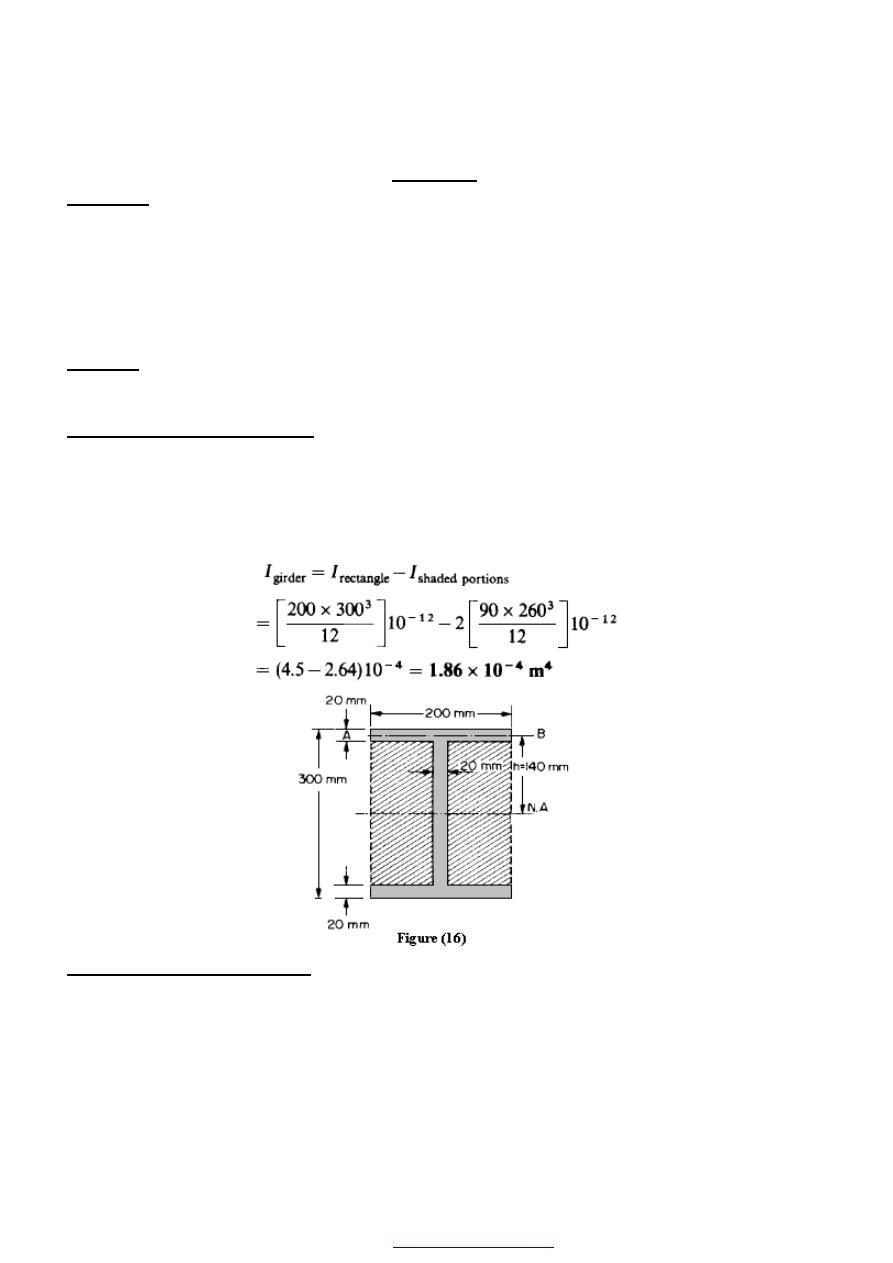
91
Examples
Example (1)
An I-section girder, 200 mm wide by 300 mm deep, with flange and web of thickness
20 mm is used as a simply supported beam over a span of 7 m. The girder carries a
distributed load of 5 kN/m and a concentrated load of 20 kN at mid-span. Determine: (a)
the second moment of area of the cross-section of the girder, (b) the maximum stress set-
up.
Solution
(a) The second moment of area of the cross-section may be found in two ways.
Method 1 -Use of standard forms
For sections with symmetry about the N.A., use can be made of the standard I value for a
rectangle about an axis through its centroid, i.e. bd
3
/12. The section can thus be divided
into convenient rectangles for each of which the N.A. passes through the centroid, e.g. in
this case, enclosing the girder by a rectangle Figure (16).
Method 2 - Parallel axis theorem
Consider the section divided into three parts - the web and the two flanges.
PDF created with pdfFactory Pro trial version
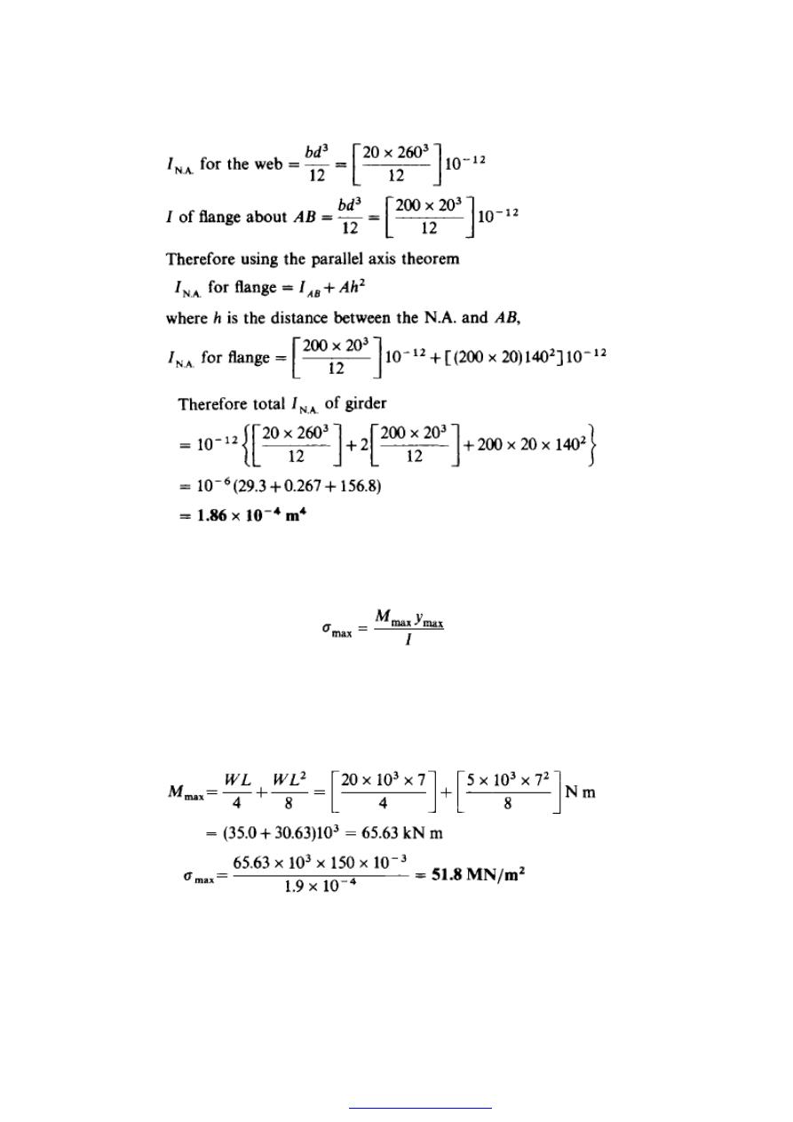
92
Both methods thus yield the same value and are equally applicable in most cases. Method
1, however, normally yields the quicker solution.
(b) The maximum stress may be found from the simple bending theory .
Now the maximum B.M. for a beam carrying a u.d.1. is at the centre and given by
(wL
2
/8). Similarly, the value for the central concentrated load is (WL/4) also at the centre.
Thus, in this case,
The maximum stress in the girder is 52 MN/m
2
, this value being compressive on the
upper surface and tensile on the lower surface.
PDF created with pdfFactory Pro trial version
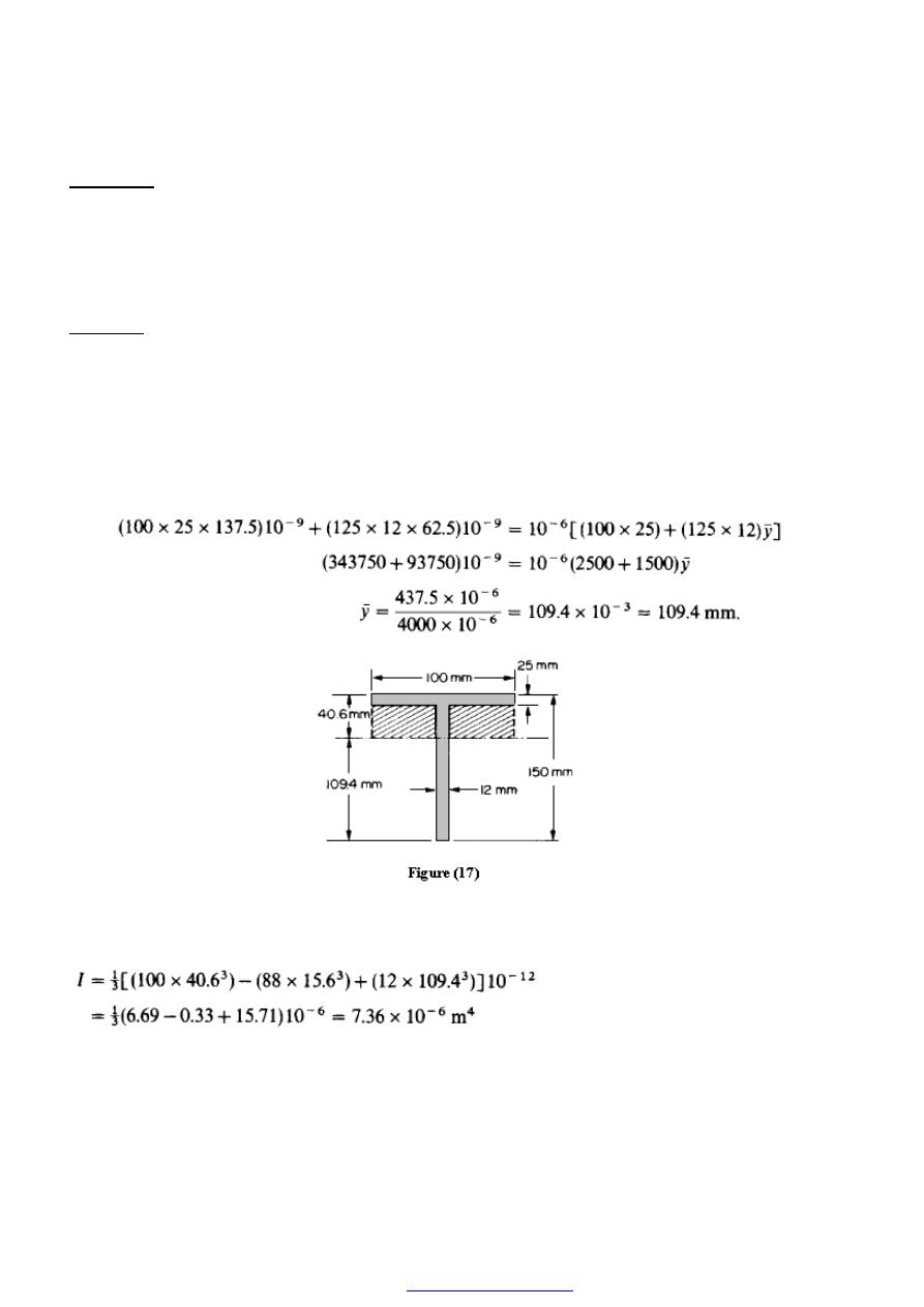
93
Example (2)
A uniform T-section beam is 100 mm wide and 150 mm deep with a flange thickness of
25 mm and a web thickness of 12 mm. If the limiting bending stresses for the material of
the beam are 80 MN/m
2
in compression and 160 MN/m
2
in tension, find the maximum
u.d.1. that the beam can carry over a simply supported span of 5 m.
Solution
The second moment of area value I used in the simple bending theory is that about the
N.A. Thus, in order to determine the I value of the T-section shown in Figure
(17), it is necessary first to position the N.A.
Since this always passes through the centroid of the section we can take moments of area
about the base to determine the position of the centroid and hence the N.A.
Thus
Thus the N.A. is positioned, as shown, a distance of 109.4 mm above the base. The
second moment of area I can now be found as suggested in Example (1) by dividing the
section into convenient rectangles with their edges in the neutral axis.
Now the maximum compressive stress will occur on the upper surface where y
= 40.6 mm, and, using the limiting compressive stress value quoted,
PDF created with pdfFactory Pro trial version
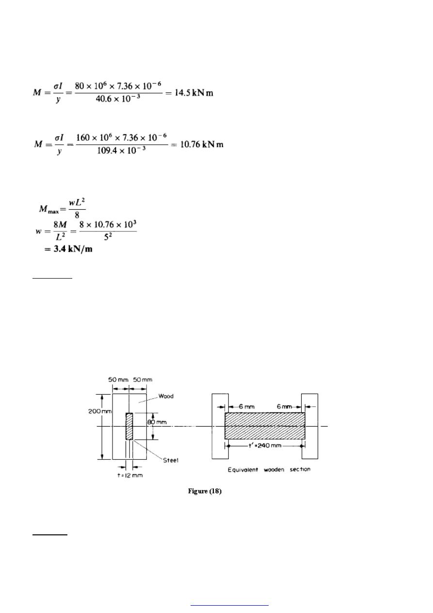
94
This suggests a maximum allowable B.M. of 14.5 kN m. It is now necessary, however, to
check the tensile stress criterion which must apply on the lower surface,
The greatest moment that can therefore be applied to retain stresses within both
conditions quoted is therefore M = 10.76 kNm. But for a simply supported beam with
u.d.l.,
The u.d.1. must be limited to 3.4 kN m.
Example (3)
A flitched beam consists of two 50 mm x 200 mm wooden beams and a 12 mm x 80 mm
steel plate. The plate is placed centrally between the wooden beams and recessed into
each so that, when rigidly joined, the three units form a 100 mm x 200 mm section as
shown in Figure(18). Determine the moment of resistance of the flitched beam when the
maximum bending stress in the timber is 12 MN/m
2
. What will then be the maximum
bending stress in the steel?
For steel E = 200 GN/m
2
; for wood E = 10 GN/m
2
.
Solution
PDF created with pdfFactory Pro trial version
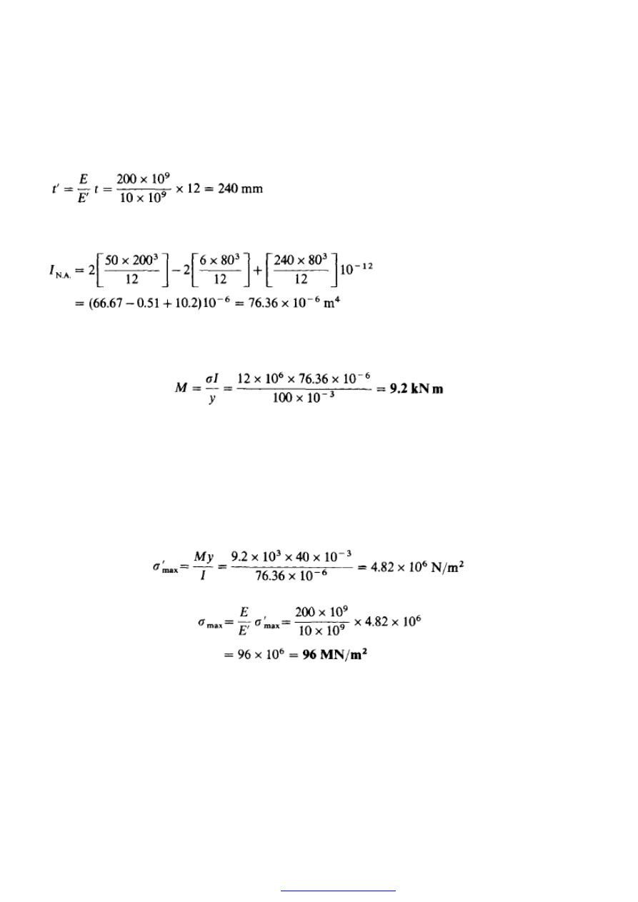
95
The flitched beam may be considered replaced by the equivalent wooden section shown
in Figure (18). The thickness t
‘ of the wood equivalent to the steel which it replaces is
given by
Then, for the equivalent section
Now the maximum stress in the timber is 12 MN/m
2
, and this will occur at y
= 100 mm; thus, from the bending theory,
The moment of resistance of the beam, i.e. the bending moment which the beam can
withstand within the given limit, is 9.2 kN m.
The maximum stress in the steel with this moment applied is then determined by finding
first the maximum stress in the equivalent wood at the same position, i.e. at y = 40 mm.
Therefore maximum stress in equivalent wood
The maximum stress in the steel is given by
PDF created with pdfFactory Pro trial version
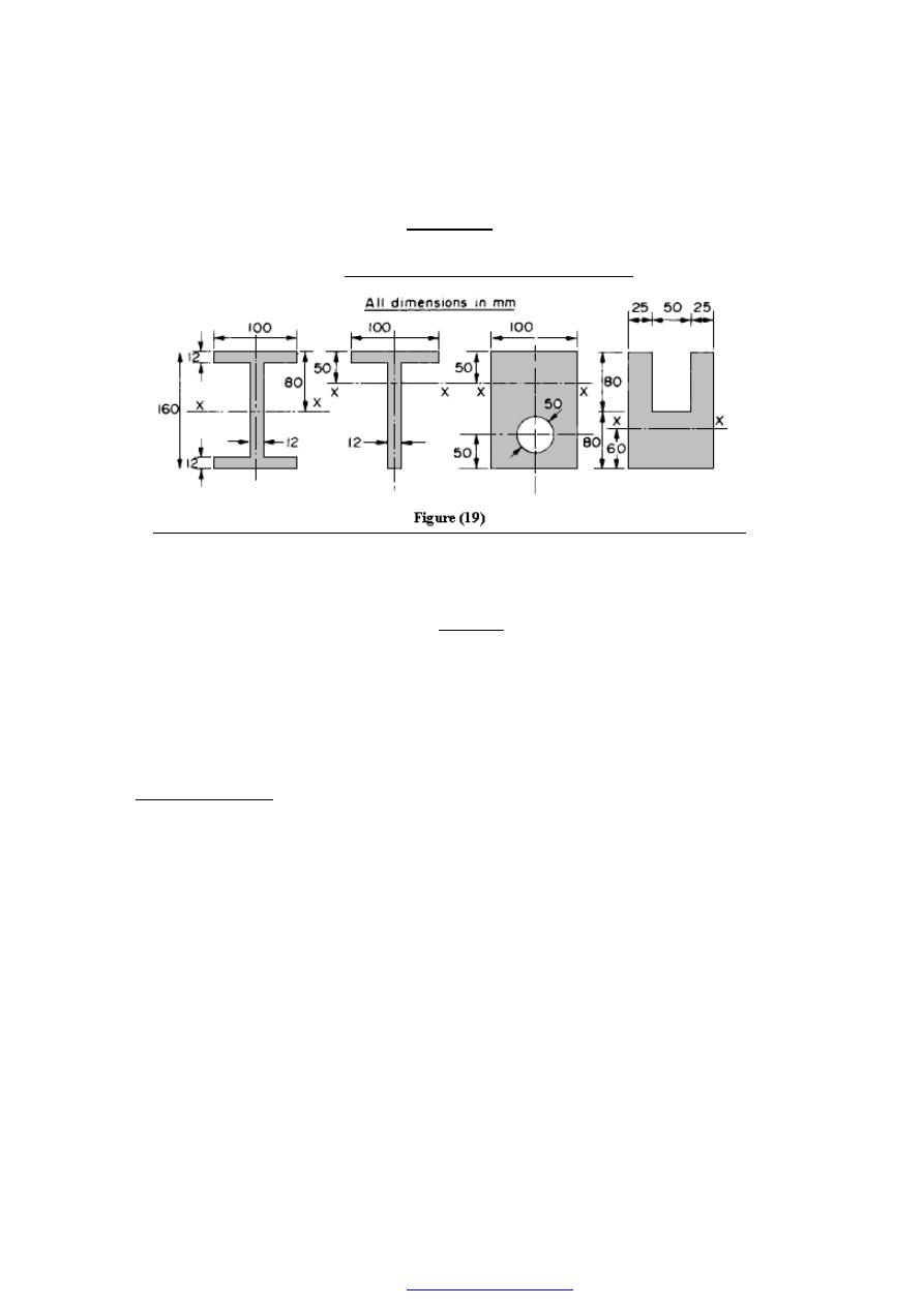
96
Problems
1 - Determine the second moments of area about the axes XX for the sections shown in
Figure (19). Ans. [15.69, 7.88, 41.15, 24; all x l0
-6
m
4
]
2- A rectangular section beam has a depth equal to twice its width. It is the same material
and mass per unit length as an I-section beam 300 mm deep with flanges 25 mm thick
and 150 mm wide and a web 12 mm thick. Compare the flexural strengths of the two
beams. Ans. [8.59: 1]
3- A conveyor beam has the cross-section shown in Figure (20) and it is subjected to a
bending moment in the plane YK Determine the maximum permissible bending
moment which can be applied to the beam (a) for bottom flange in tension, and (b) for
bottom flange in compression, if the safe stresses for the material in tension and
compression
are
30
MN/m
2
and
150
MN/m
2
respectively.
Ans.[32.3, 84.8 kN m.]
PDF created with pdfFactory Pro trial version
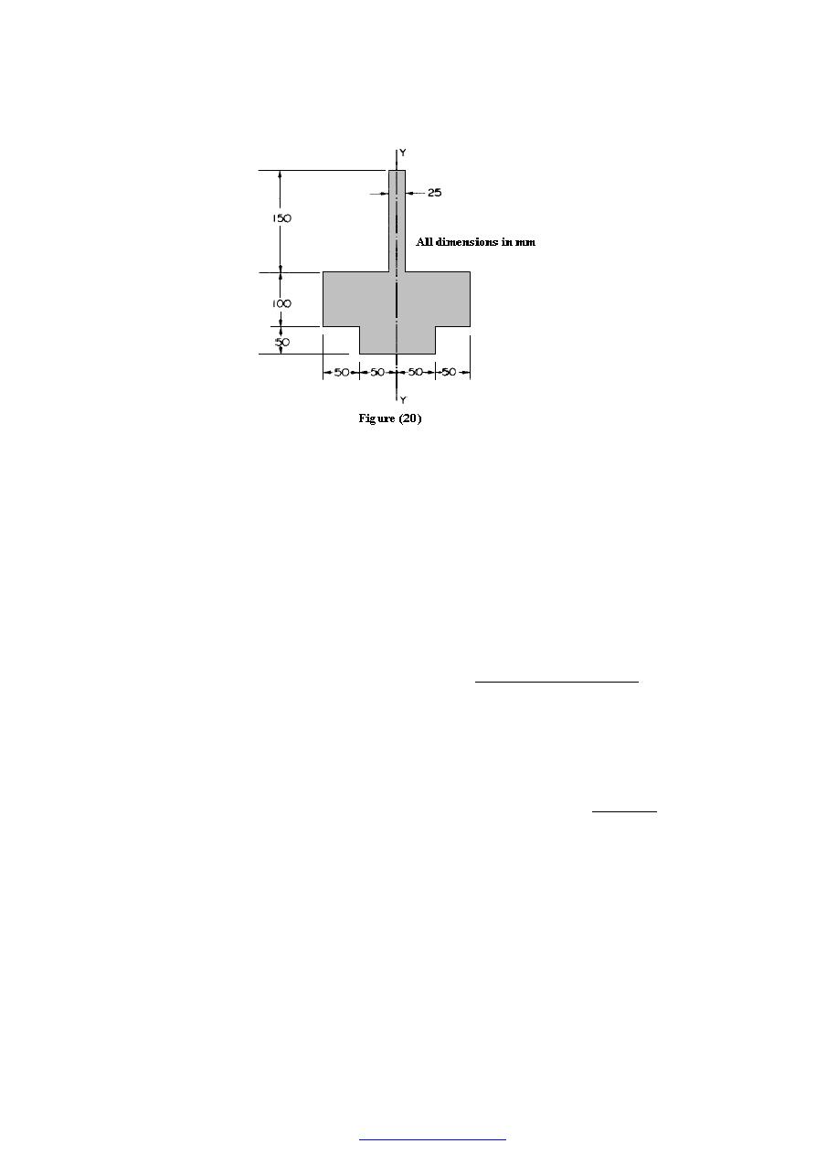
97
4- A horizontal steel girder has a span of 3 m and is built-in at the left-hand end and
freely supported at the other end. It carries a uniformly distributed load of 30
kN/m over the whole span, together with a single concentrated load of 20 kN at a
point 2 m from the left-hand end. The supporting conditions are such that the reaction
at the left-hand end is 65 kN.
(a) Determine the bending moment at the left-hand end and draw the B.M.
diagram.
(b) Give the value of the maximum bending moment.
(c) If the girder is 200 mm deep and has a second moment of area of 40 x 10
-6
m
4
determine the maximum stress resulting from bending.
Ans. [40 kN m; 100 MN/m
2
]
5- Figure (21) represents the cross-section of an extruded alloy member which acts as a
simply supported beam with the 75 mm wide flange at the bottom. Determine the
moment of resistance of the section if the maximum permissible stresses in tension
and compression are respectively 60 MN/m
2
and 45 MN/m
2
.
Ans.[62 kN m]
PDF created with pdfFactory Pro trial version
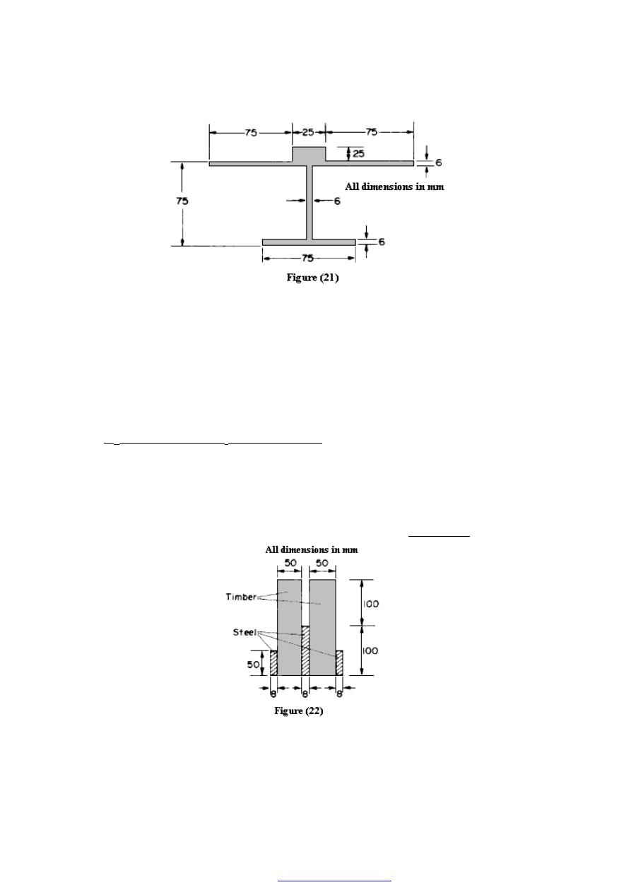
98
6- A brass strip, 50 mm x 12 mm in section, is riveted to a steel strip, 65
mm x 10 mm in section, to form a compound beam of total depth 22 mm, the brass
strip being on top and the beam section being symmetrical about the vertical axis. The
beam is simply supported on a span of 1.3 m and carries a load of 2 kN at mid-span.
(a) Determine the maximum stresses in each of the materials owing to bending.
(b) Make a diagram showing the distribution of bending stress over the depth of the
beam. Take E for steel = 200 GN/m
2
and E for brass = 100 GN/m
2
.
Ans.[
σ
b
= 130 MN/m
2
;
σ
s
= 162.9 MN/m
2
]
7- A composite beam is of the construction shown in Figure (22). Calculate the allowable
u.d.1. that the beam can carry over a simply supported span of 7 m if the stresses are
limited to 120 MN/m
2
in the steel and 7 MN/m
2
in the timber.
Modular ratio = 20. Ans.[ 1.13 kN/m.]
8- Two bars, one of steel, the other of aluminium alloy, are each of 75 mm width and are
rigidly joined together to form a rectangular bar 75 mm wide and of depth (t
s
+ t
A
),
PDF created with pdfFactory Pro trial version

99
where t
s
= thickness of steel bar and t
A
= thickness of alloy bar. Determine the ratio
oft, to t,, in order that the neutral axis of the compound bar is coincident with the
junction of the two bars. (E
s
= 210 GN/m
2
; E
A
= 70 GN/m
2
) If
such a beam is 50 mm deep determine the maximum bending moment the beam can
withstand if the maximum stresses in the steel and alloy are limited to 135 MN/m
2
and 37 MN/m
2
respectively.
Ans.[0.577; 1.47 kNm.]
PDF created with pdfFactory Pro trial version
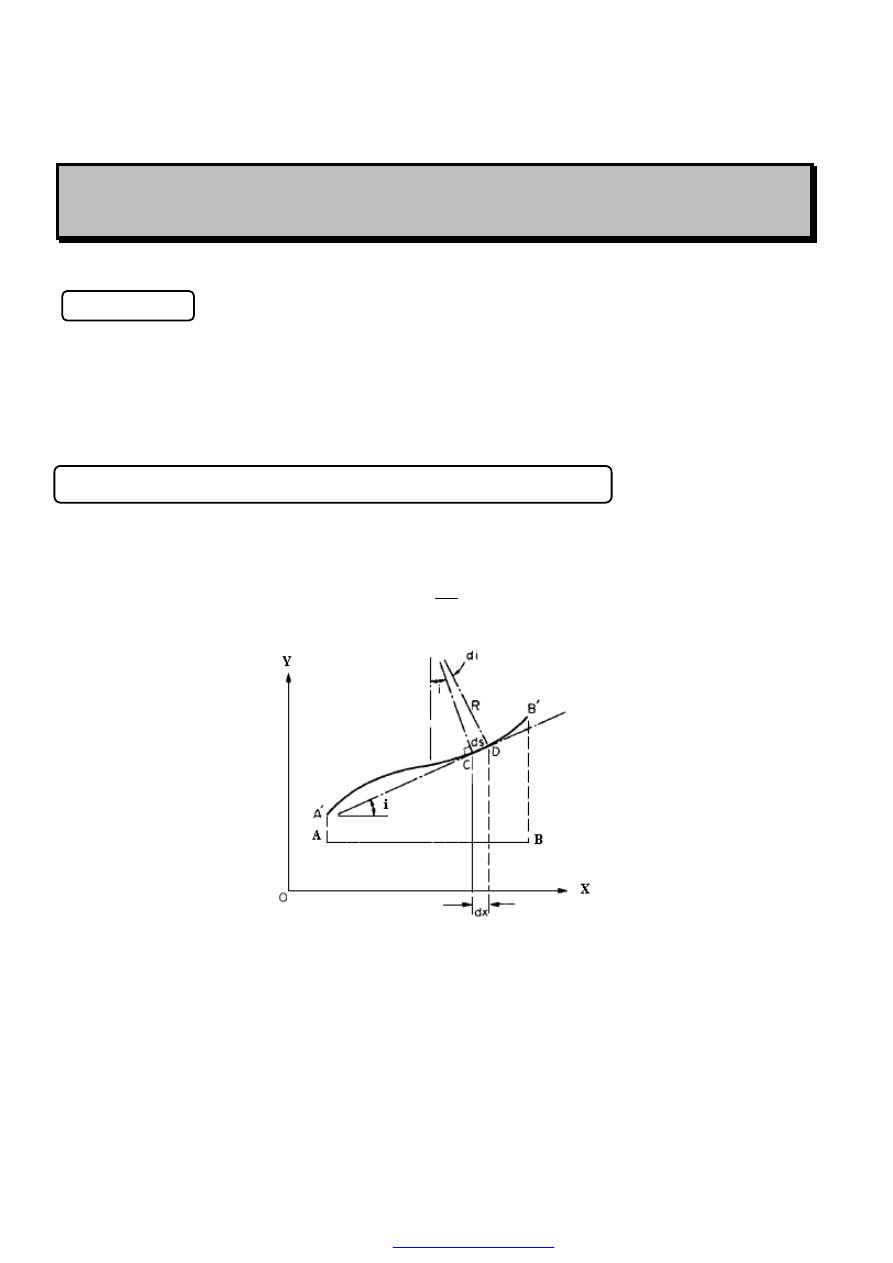
100
S
S
L
L
O
O
P
P
E
E
A
A
N
N
D
D
D
D
E
E
F
F
L
L
E
E
C
C
T
T
I
I
O
O
N
N
O
O
F
F
B
B
E
E
A
A
M
M
S
S
Introduction
In practically all engineering applications limitations are placed upon the
performance and behavior of components and normally they are expected to operate
within certain set limits of for example, stress or deflection. The stress limits are normally
set so that the component does not yield or fail under the most severe load conditions
which it is likely to meet in service.
Relationship between loading, S.F., B.M., slope and deflection
Consider a beam (AB) which is initially horizontal when unloaded. If this deflects to a
new position (A
/
B
/
) under load, the slope at any point C is
dx
dy
i
=
Figure (1) Unloaded beam AB deflected to A
/
B
/
under load
This is usually very small in practice, and for small curvatures
PDF created with pdfFactory Pro trial version
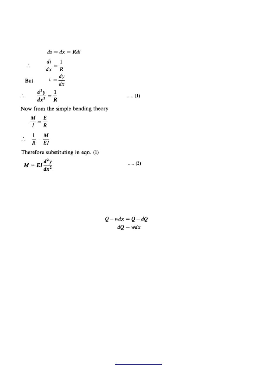
101
This is the basic differential equation for the deflection of beams.
If the beam is now assumed to carry a distributed loading which varies in intensity
over the length of the beam, then a small element of the beam of length (dx) will be
subjected to the loading condition shown in Figure (2). The parts of the beam on either
side of the element (EFGH) carry the externally applied forces, while reactions to these
forces are shown on the element itself. Thus for vertical equilibrium of (EFGH),
PDF created with pdfFactory Pro trial version
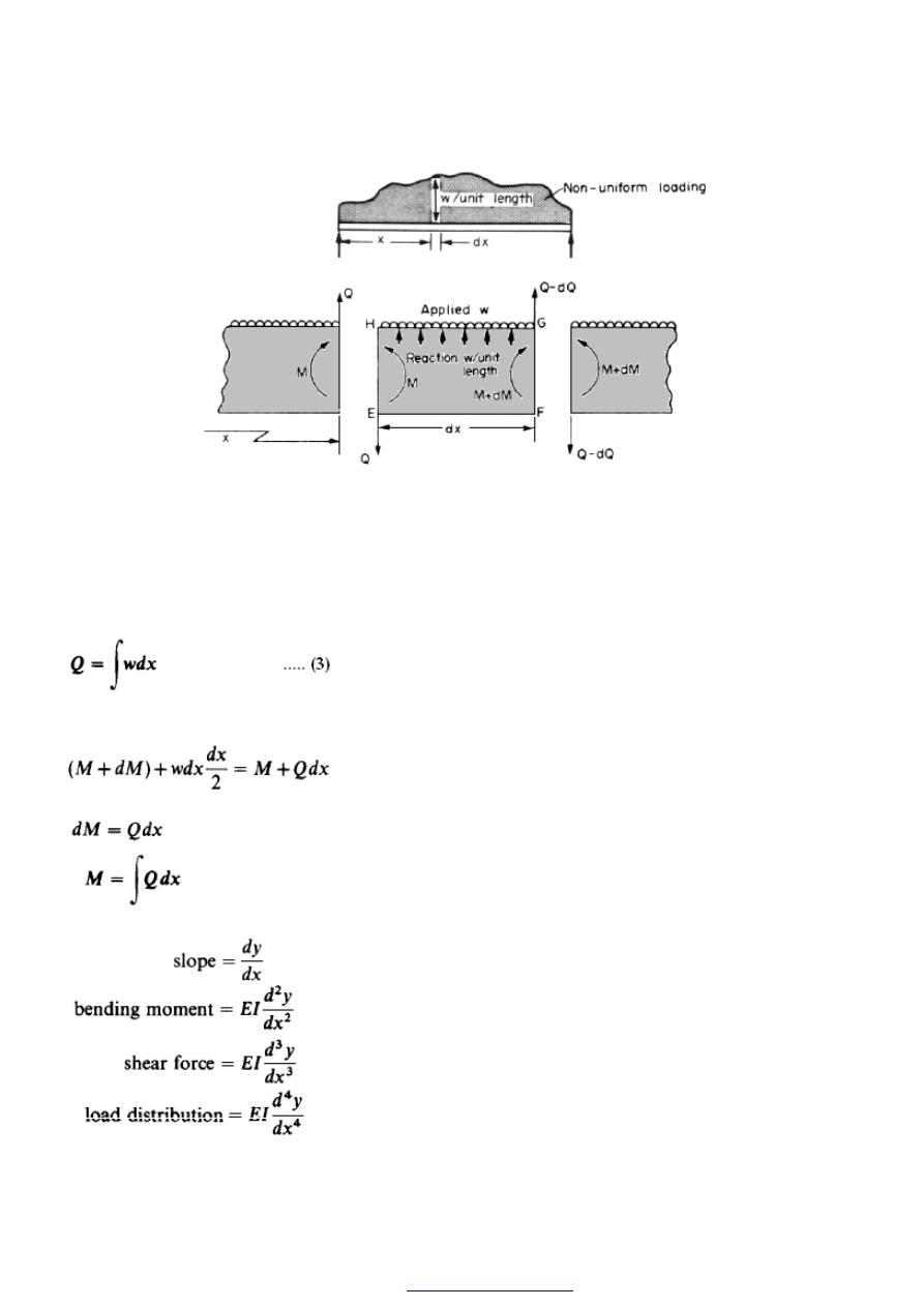
102
Figure (2) Small element of beam subjected to non-uniform loading
(effectively uniform over small length dx).
and integrating,
Also, for equilibrium, moments about any point must be zero.
Therefore taking moments about F,
Therefore neglecting the square of small quantities,
deflection = y
PDF created with pdfFactory Pro trial version
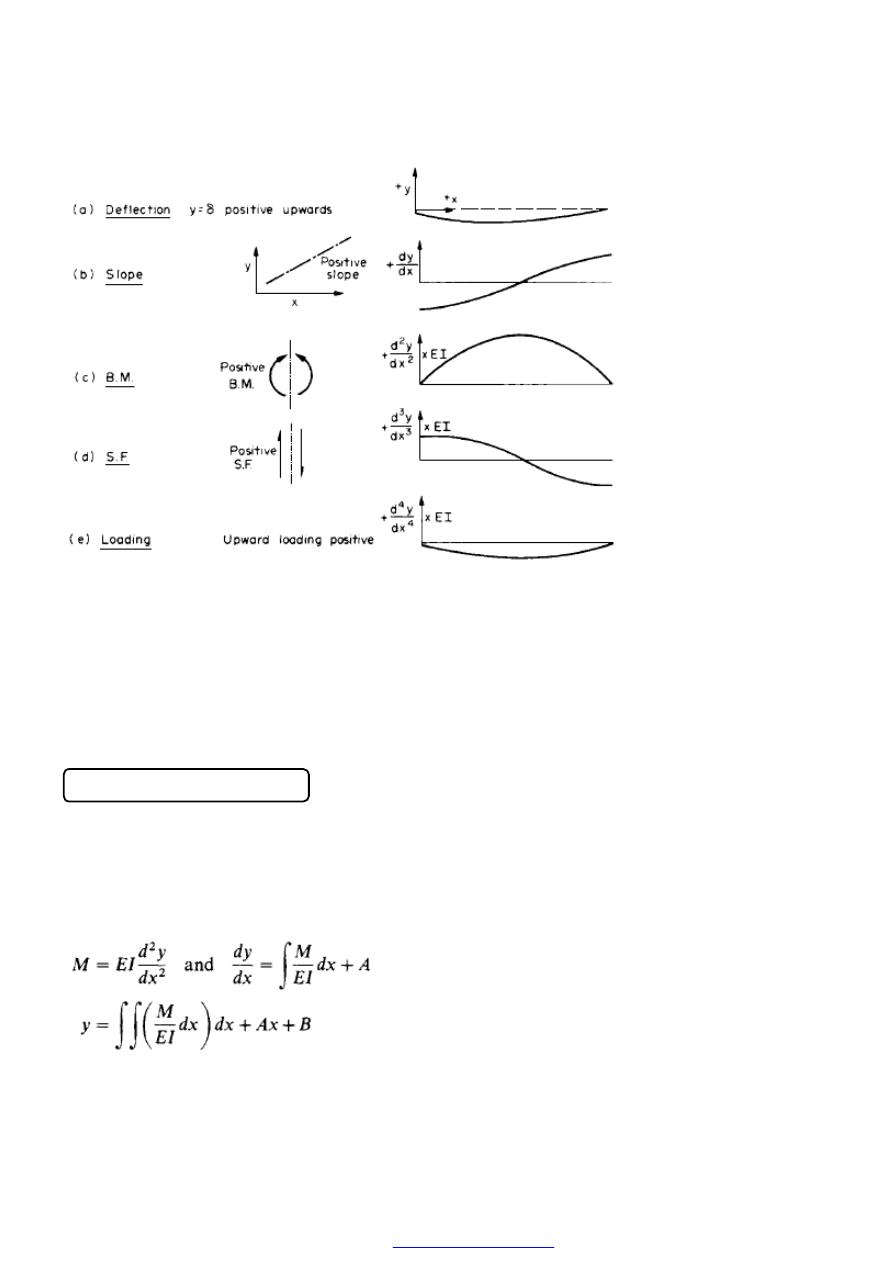
103
Figure (3) Sign conventions for load, S.F., B.M., slope and deflection.
In order that the above results should agree algebraically, i.e. that positive slopes shall
have the normal mathematical interpretation of the positive sign and that B.M. and S.F.
conventions are consistent with those introduced earlier, it is imperative that the sign
convention illustrated in Figure (3) be adopted.
Direct integration method
If the value of the B.M. at any point on a beam is known in terms of x, the distance
along the beam, and provided that the equation applies along the complete beam, then
integration of eqn. (5.4a) will yield slopes and deflections at any point,
i.e.
PDF created with pdfFactory Pro trial version
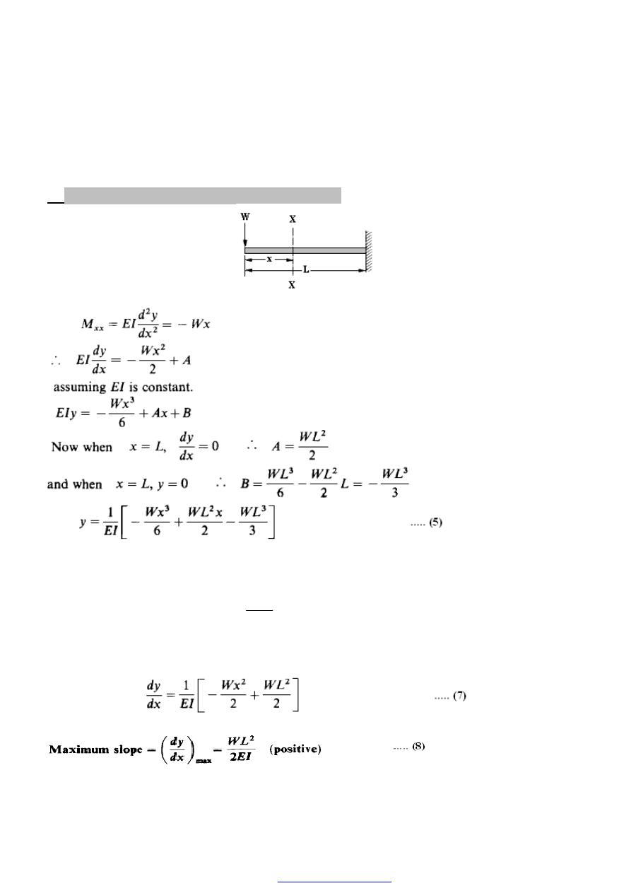
104
where A and B are constants of integration evaluated from known conditions of slope and
deflection for particular values of x.
(a) Cantilever with concentrated load at the end
Figure (4)
This gives the deflection at all values of x and produces a maximum value at the tip of the
cantilever when x = 0,
I
E
L
W
y
deflection
Maximum
.
3
.
3
.
max
−
=
=
…… (6)
The negative sign indicates that deflection is in the negative y direction, i.e. downwards.
and produces a maximum value again when x = 0.
PDF created with pdfFactory Pro trial version
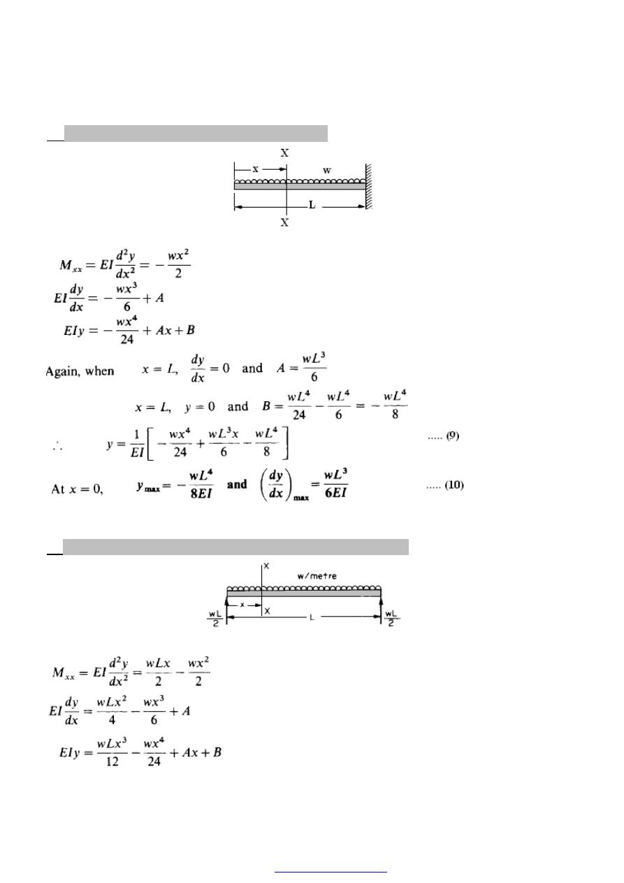
105
(b) Cantilever with uniformly distributed load
Figure (5)
(c) Simply-supported beam with uniformly distributed load
Figure (6)
PDF created with pdfFactory Pro trial version
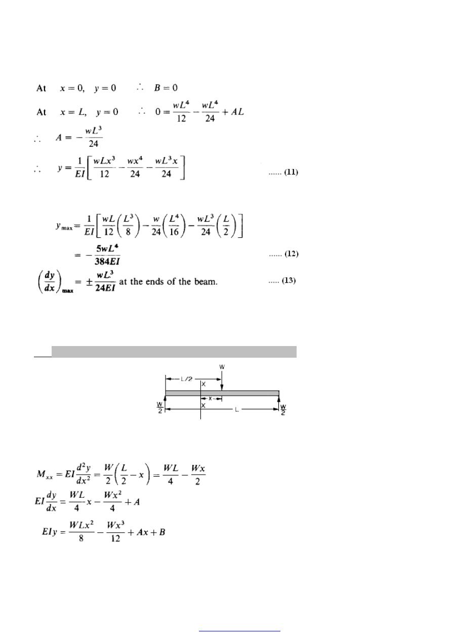
106
In this case the maximum deflection will occur at the centre of the beam where
x = L/2.
( d ) Simply supported beam with central concentrated load
Figure (7)
In order to obtain a single expression for B.M. which will apply across the complete
beam in this case it is convenient to take the origin for x at the centre, then:
PDF created with pdfFactory Pro trial version
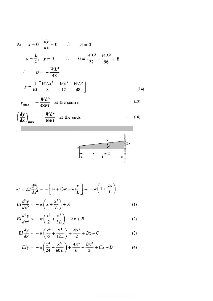
107
(e) Cantilever subjected to non-uniform distributed load
Figure (8)
The loading at section X X is
PDF created with pdfFactory Pro trial version
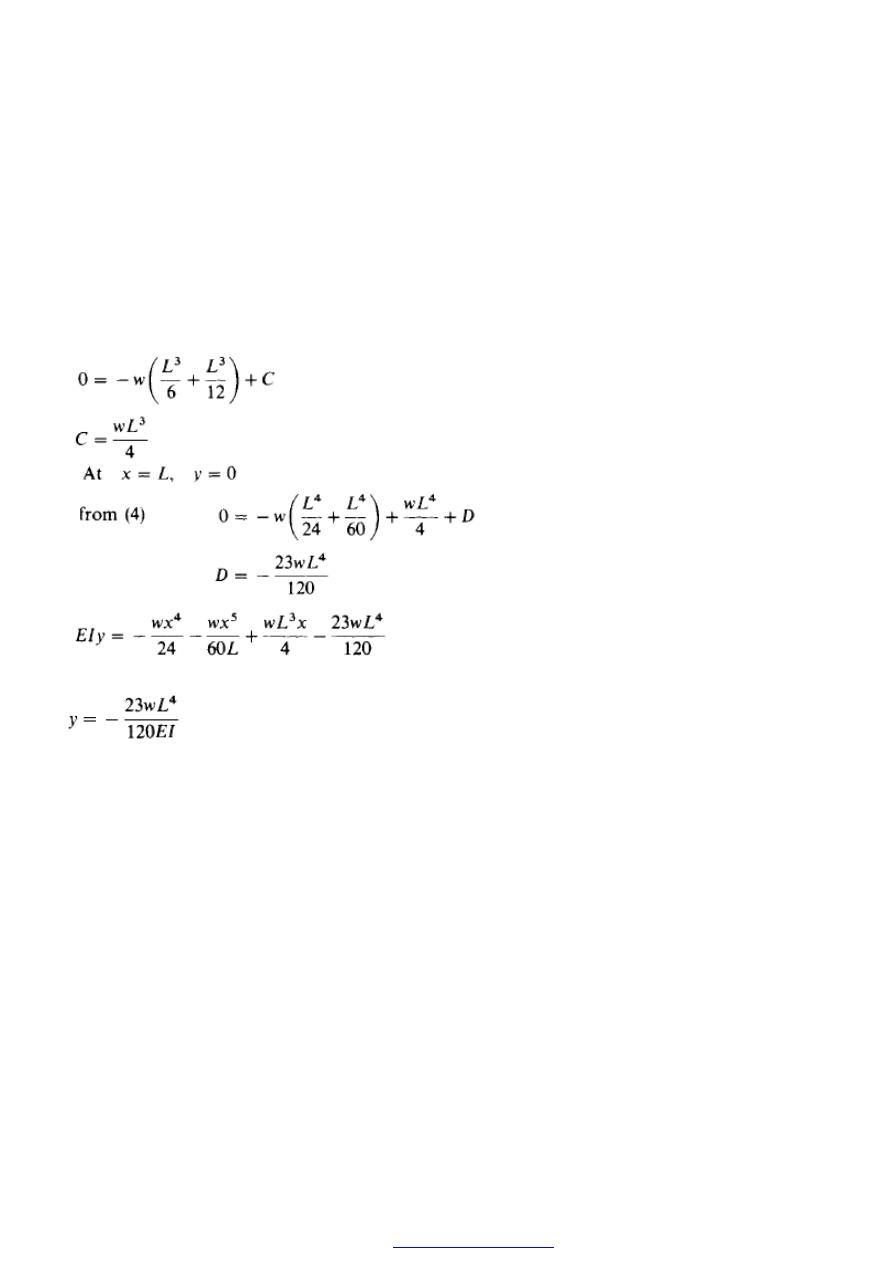
108
Thus, before the slope or deflection can be evaluated, four constants have to be
determined; therefore four conditions are required. They are:
At x = 0, S.F. is zero
from (1); A = O
At x = 0, B.M. is zero
from (2); B = O
At x = L, slope dy/dx = 0 (slope normally assumed zero at a built-in support)
from (3)
Then, for example, the deflection at the tip of the cantilever, where x = 0, is
PDF created with pdfFactory Pro trial version
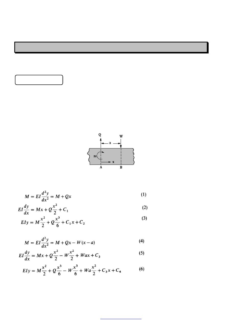
109
S
S
L
L
O
O
P
P
E
E
A
A
N
N
D
D
D
D
E
E
F
F
L
L
E
E
C
C
T
T
I
I
O
O
N
N
O
O
F
F
B
B
E
E
A
A
M
M
S
S
Macaulay’s method
The simple integration method used in the previous examples can only be used when
a single expression for B.M. applies along the complete length of the beam. In general
this is not the case, and the method has to be adapted to cover all loading conditions.
Consider, therefore, a small portion of a beam in which, at a particular section A, the
shearing force is Q and the B.M. is M, as shown in Figure (9 ). At another section B,
distance a along the beam, a concentrated load W is applied which will change the B.M.
for points beyond B.
Figure (9)
Between A and B,
Beyond, B
PDF created with pdfFactory Pro trial version
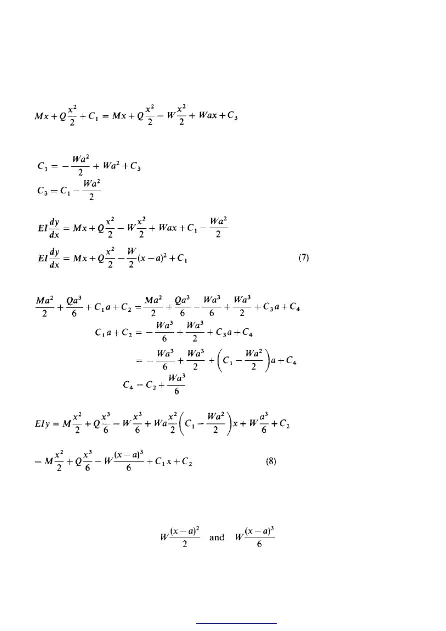
110
Now for the same slope at B, equating (2) and (5),
But at B, x = a
Substituting in (5)
Also, for the same deflection at (B) equating (3) and (6), with x = a
Substituting in (6),
Thus, inspecting (4), (7) and (8), we can see that the general method of obtaining slopes
and deflections (i.e. integrating the equation for M ) will still apply provided that the term
W(x -a) is integrated with respect to (x -a) and not x. Thus, when integrated, the term
becomes
PDF created with pdfFactory Pro trial version
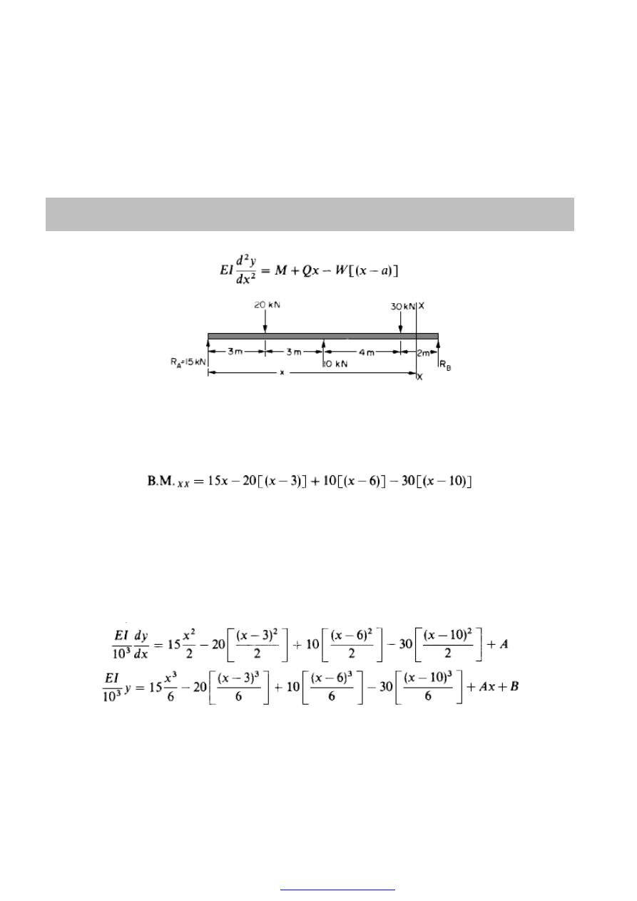
111
successively.
In addition, since the term W(x - a) applies only after the discontinuity,
i.e. when x > a, it should be considered only when x > a or when (x - a) is positive. For
these reasons such terms are conventionally put into square or curly brackets and called
Macaulay terms.
Thus Macaulay terms must be (a) integrated with respect to themselves and (b)
neglected when negative.
For the whole beam, therefore,
Figure (10)
As an illustration of the procedure consider the beam loaded as shown in
Figure (10)
for which the central deflection is required. Using the Macaulay method the equation for
the B.M. at any general section XX is then given by
Care is then necessary to ensure that the terms inside the square brackets (Macaulay
terms) are treated in the special way noted on the previous page.
Here it must be emphasised that all loads in the right-hand side of the equation are in
units of kN (i.e. newtons X l0
3
).I n subsequent working, therefore, it is convenient to
carry through this factor as a denominator on the left-hand side in order that the
expressions are dimensionally correct.
Integrating,
where A and B are two constants of integration.
Now when x =0, y = 0 .’. B = 0
and when x = 12, y = 0
PDF created with pdfFactory Pro trial version
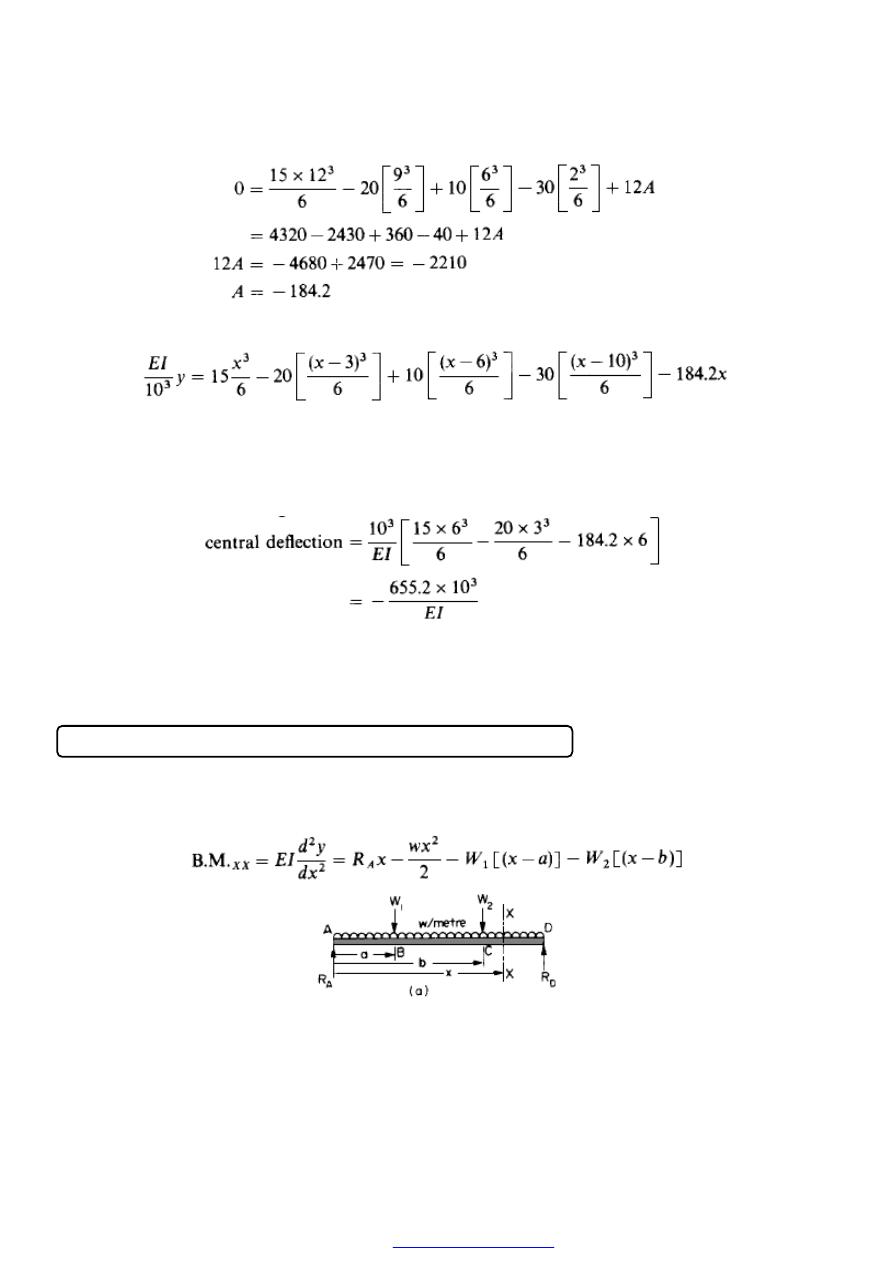
112
The deflection at any point is given by
The deflection at mid-span is thus found by substituting x = 6 in the above equation,
bearing in mind that the dimensions of the equation are kN.m
3
.
N.B.-Two of the Macaulay terms then vanish since one becomes zero and the other
negative and therefore neglected.
With typical values of E = 208 GN/m
2
and I = 82 x m
4
central deflection = 38.4 x l0-3 m = 38.4 mm
Macaulay’s method for uniformly distributed load (u.d.l)
If a beam carries a uniformly distributed load over the complete span as shown in
Figure (11a).
PDF created with pdfFactory Pro trial version
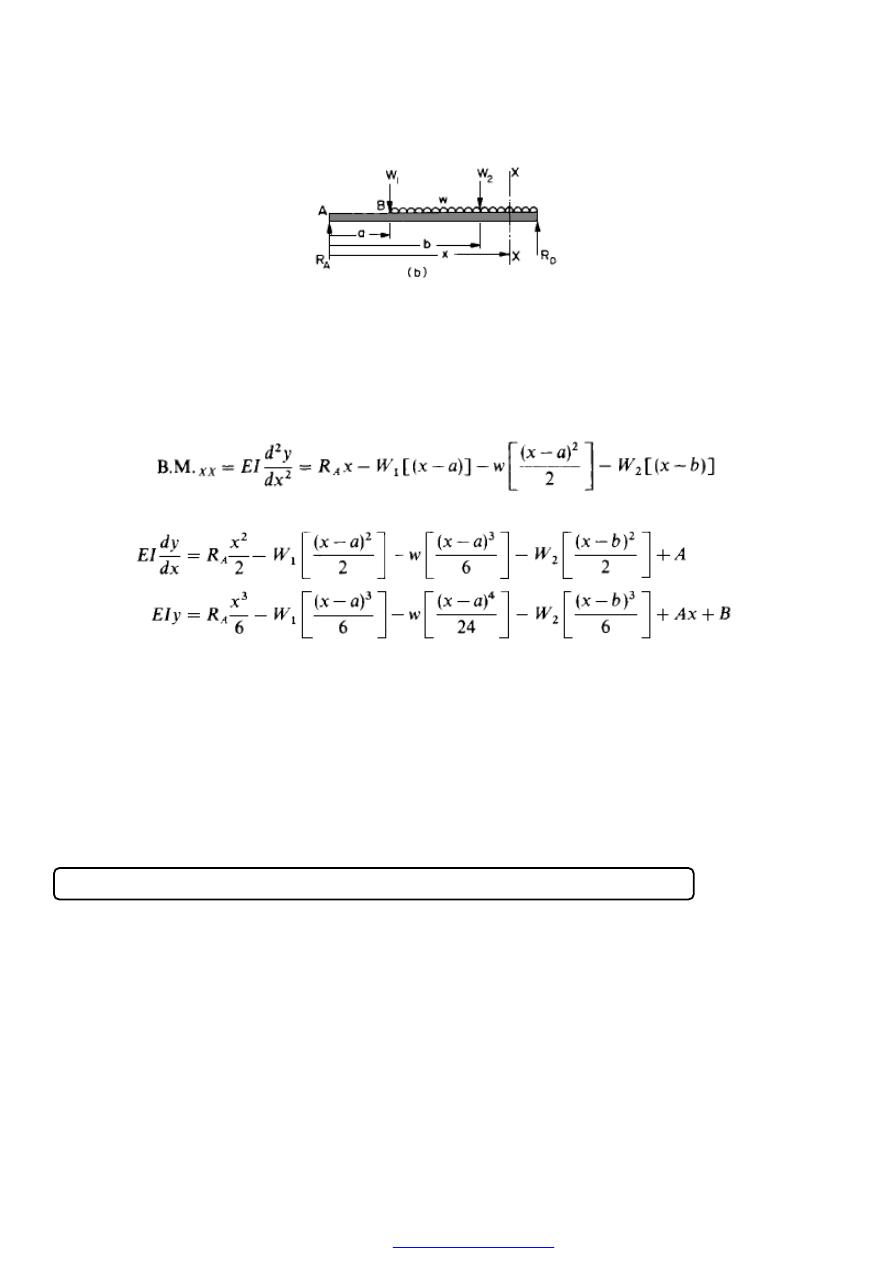
113
Figure (11)
The u.d.l. term applies across the complete span and does not require the special
treatment associated with the Macaulay terms. If, however, the u.d.1. starts at B as
shown in Figure (11b) the B.M. equation is modified and the u.d.1. term becomes a
Macaulay term and is written inside square brackets.
Integrating,
Note that Macaulay terms are integrated with respect to, for example, (x -a) and they
must be ignored when negative. Substitution of end conditions will then yield the values
of the constants A and B in the normal way and hence the required values of slope or
deflection. It must be appreciated, however, that once a term has been entered in the B.M.
expression it will apply across the complete beam. The modifications to the procedure
required for cases when u.d.1.s. are applied over part of the beam only are introduced in
the following theory.
Macaulay's method for beams with u.d.1. applied over part of the beam
Consider the beam loading case shown in Figure (12).
PDF created with pdfFactory Pro trial version
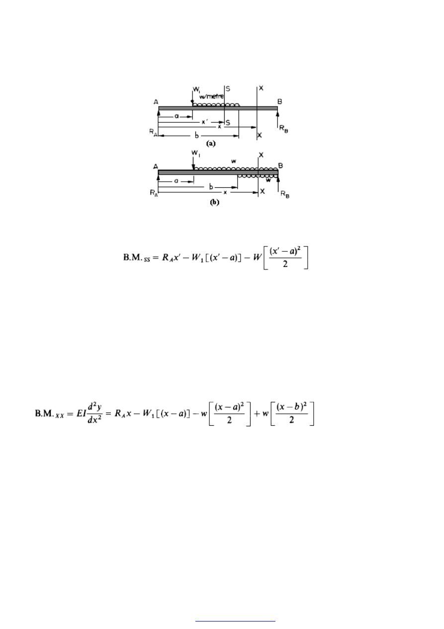
114
Figure (12)
The B.M. at the section SS is given by the previously introduced procedure as
Having introduced the last (u.d.1.) term, however, it will apply for all values of x'
greater than a, i.e. across the rest of the span to the end of the beam. (Remember,
Macaulay terms are only neglected when they are negative, e.g. with x' < a.) The above
equation is NOT therefore the correct equation for the load condition shown. The
Macaulay method requires that this continuation of the u.d.1. be shown on the loading
diagram and the required loading condition can therefore only be achieved by introducing
an equal and opposite u.d.1. over the last part of the beam to cancel the unwanted
continuation of the initial distributed load. This procedure is shown in Figure (12b).
The correct B.M. equation for any general section XX is then given by
This type of approach can be adopted for any beam loading cases in which u.d.1.s are
stopped or added to.
Example (1)
Determine the deflection at a point 1 m from the left-hand end of the beam loaded as
shown in Figure (13a) using Macaulay’s method. EI = 0.65 MN m
2
.
PDF created with pdfFactory Pro trial version
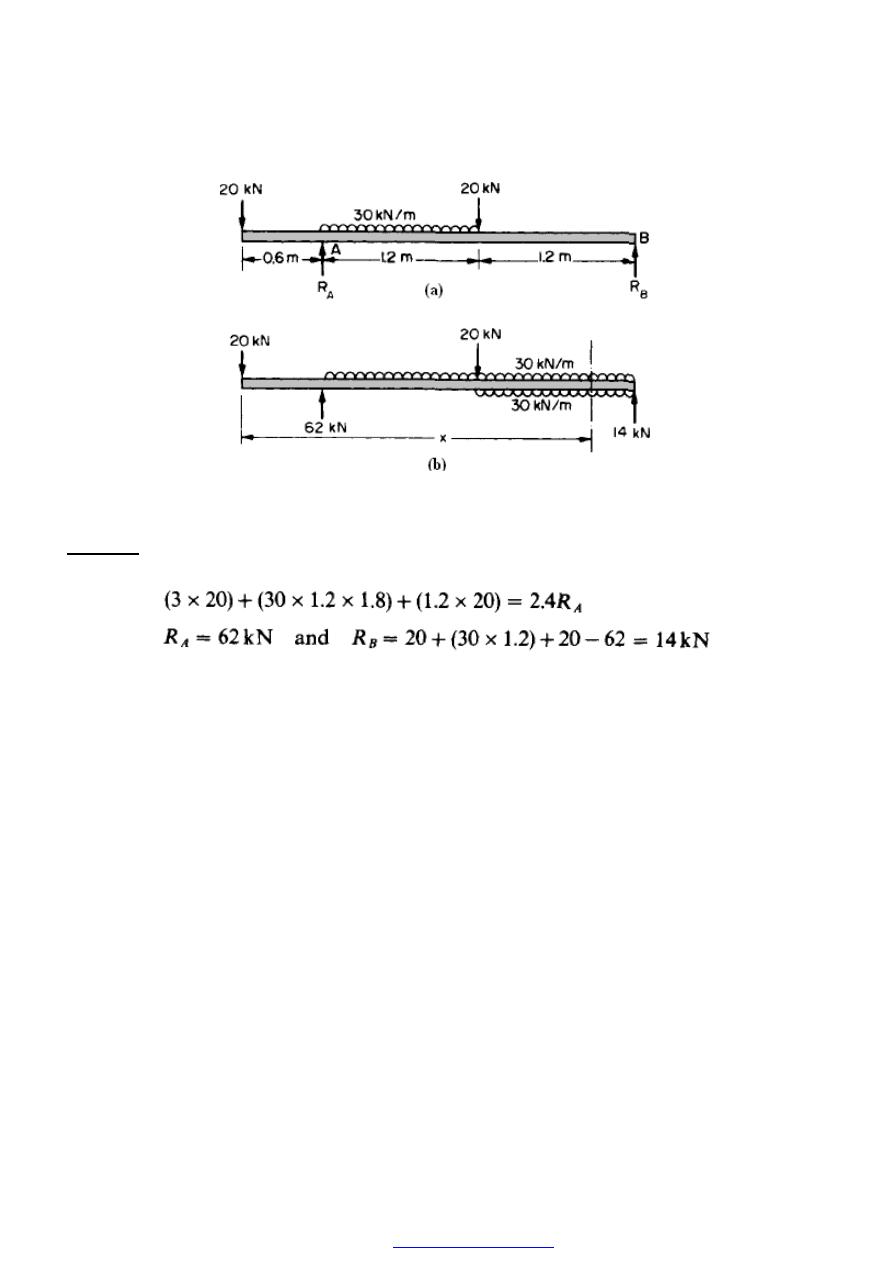
115
Figure (13)
Solution
Taking moments about B
Using the modified Macaulay approach for distributed loads over part of a beam
introduced in Figure (13b),
PDF created with pdfFactory Pro trial version
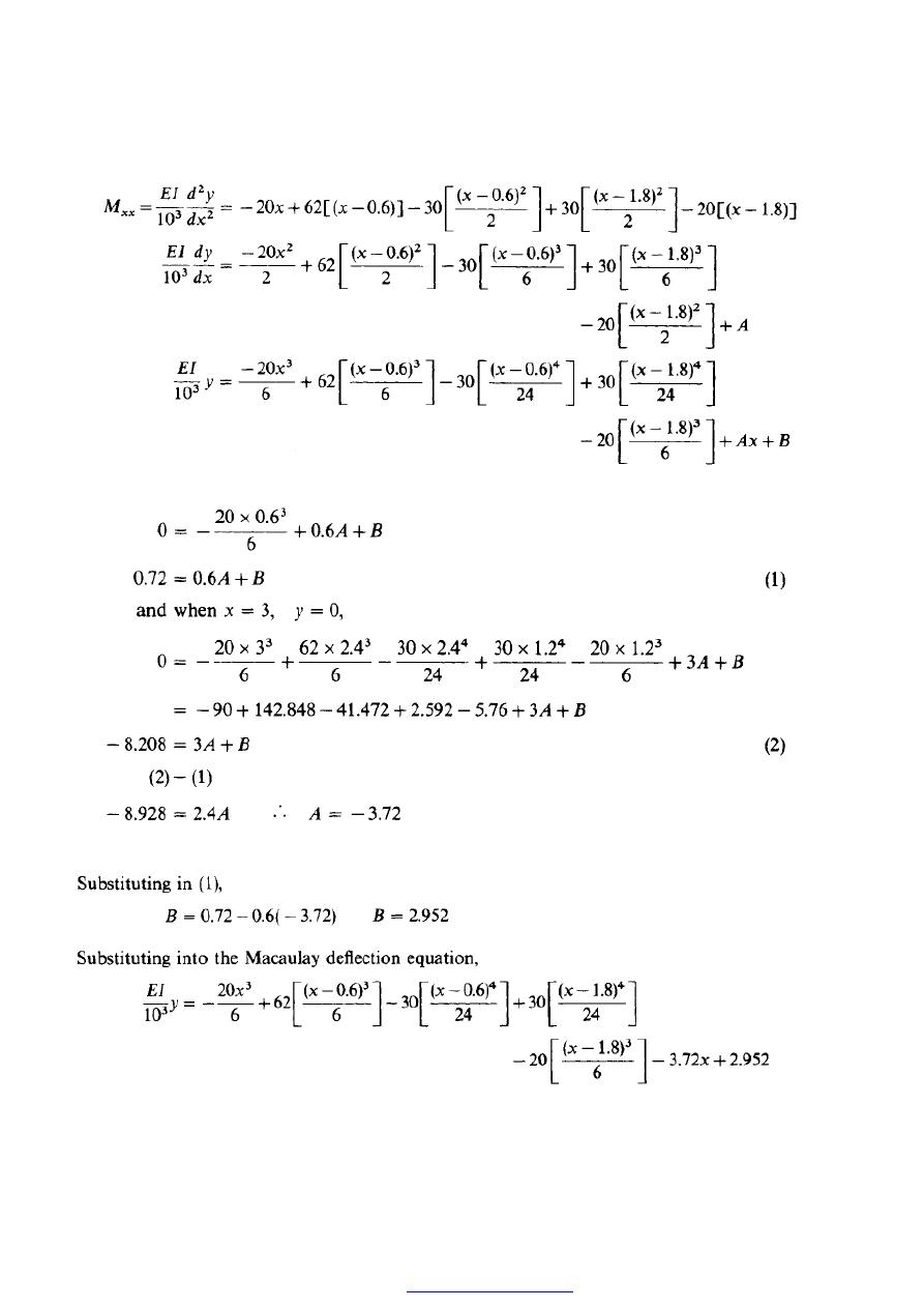
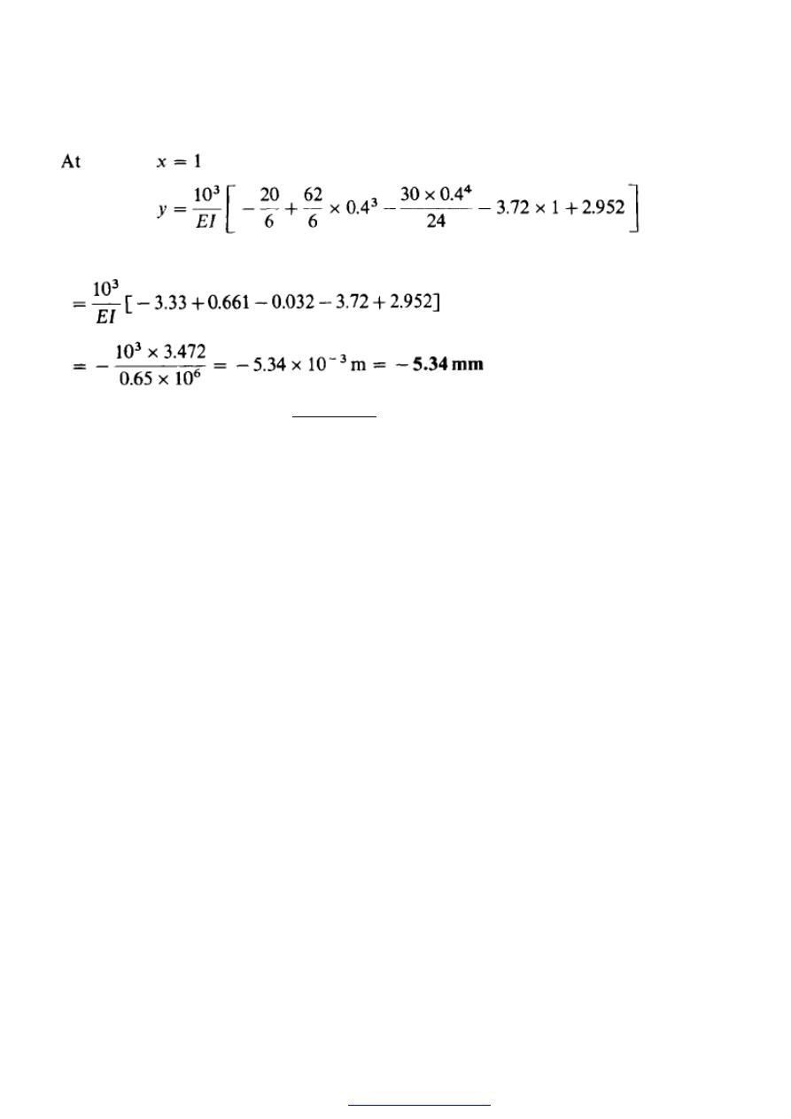
117
In order that the above results should, i.e. that positive slopes shall have the
The beam therefore is deflected downwards at the given position.
PDF created with pdfFactory Pro trial version
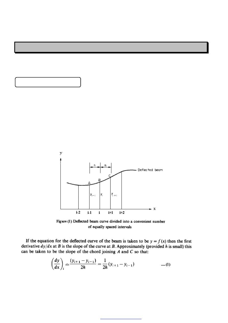
118
S
S
L
L
O
O
P
P
E
E
A
A
N
N
D
D
D
D
E
E
F
F
L
L
E
E
C
C
T
T
I
I
O
O
N
N
O
O
F
F
B
B
E
E
A
A
M
M
S
S
3- Finite difference method
A numerical method for the calculation of beam deflections which is particularly useful
for non-prismatic beams or for cases of irregular loading is the so-called finite difference
method. The basic principle of the method is to replace the standard differential equation
(1) by its finite difference approximation, obtain equations for deflections in terms of
moments at various points along the beam and solve these simultaneously to yield the
required deflection values.
Consider, therefore, Figure (1) which shows part of a deflected beam with the x-
axis divided into a series of equally spaced intervals. By convention, the ordinates are
numbered with respect to the Central ordinate B.
.
PDF created with pdfFactory Pro trial version
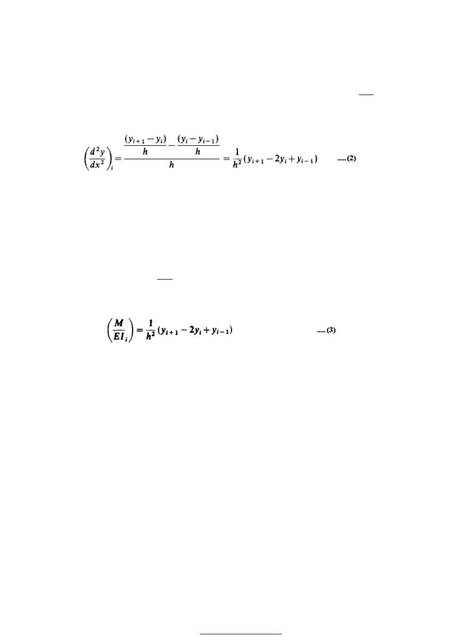
119
The rate of change of the first derivative, i.e. the rate of change of the slope
2
2
dx
y
d
=
given in the same way approximately as the slope to the right of (i) minus the slope to the
left of (i) divided by the interval between them.
Equations (1) and (2) are the finite difference approximations of the standard beam
deflection differential equations and, because they are written in terms of ordinates on
either side of the central point (i), they are known as central differences. Alternative
expressions which can be formed to contain only ordinates at, or to the right of (i), or
ordinates at, or to the left of (i) are known as forward and backward differences,
respectively but these will not be considered here.
Now from equation ,
2
2
dx
y
d
EI
M
=
.'. At position (i), combining equations between above equation and equation (2).
A solution for any of the deflection (y) values can then be obtained by applying the finite
difference equation at a series of points along the beam and solving the resulting
simultaneous equations. The higher the number of points selected the greater the
accuracy of solution but the more the number of equations which are required to be
solved. The method thus lends itself to computer-assisted evaluation. In addition to the
solution of statically determinate beam problems of the type treated in example (1) the
method is also applicable to the analysis of statically indeterminate beams.
The principal advantages of the finite difference method are thus:
(a) that it can be applied to statically determinate or indeterminate beams,
(b) that it can be used for non-prismatic beams,
(c) that it is amenable to computer solutions.
PDF created with pdfFactory Pro trial version
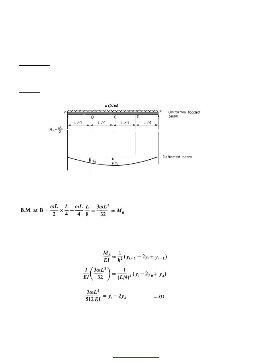
120
Example (1)
Using the finite difference method, determine the central deflection of a
simply-supported beam carrying a uniformly distributed load over its complete span. The
beam can be assumed to have constant flexural rigidity El throughout.
Solution
As a simple demonstration of the finite difference approach, assume that the beam is
divided into only four equal segments (thus reducing the accuracy of the solution from
that which could be achieved with a greater number of segments).
The n,
but, from equation (3)
and, since y, = 0,
PDF created with pdfFactory Pro trial version
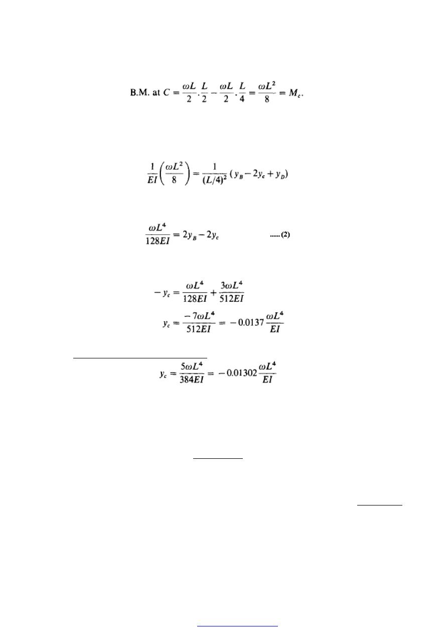
121
and, from equation (3)
Now, from symmetry, y
D
= y
B
Adding eqns. (1) and (2);
the negative sign indicating a downwards deflection as expected. This value compares
with the "exact method (by direct method)" value of:
a difference of about 5 %. As stated earlier, this comparison could be improved by
selecting more segments but, nevertheless, it is remarkably accurate for the very small
number of segments chosen.
Problems
1-A beam of length 10 m is symmetrically placed on two supports 7m apart. The loading
is 15 kN/m between the supports and 20 kN at each end. What is the central deflection
of the beam? E = 210 GN/m
2
; I = 200 x 10
-6
m
4
.
Ans. [6.8 mm.]
2-Derive the expression for the maximum deflection of a simply supported beam of
negligible weight carrying a point load at its mid-span position. The distance between
PDF created with pdfFactory Pro trial version

122
the supports is L, the second moment of area of the cross-section is (I) and the modulus
of elasticity of the beam material is (E).
The maximum deflection of such a simply supported beam of length 3 m is 4.3 mm
when carrying a load of 200 kN at its mid-span position. What would be the deflection
at the free end of a cantilever of the same material, length and cross-section if it carries
a load of l00kN at a point 1.3m from the free end? Ans.[13.4
mm]
3-A horizontal beam, simply supported at its ends, carries a load which varies uniformly
from 15 kN/m at one end to 60 kN/m at the other. Estimate the central deflection if the
span is 7 m, the section 450 mm deep and the maximum bending stress 100 MN/m
2
, E
= 210 GN/m
2
. Ans. [21.9 mm.]
4-A beam AB, 8 m long, is freely supported at its ends and carries loads of 30 kN and 50
kN at points 1 m and 5 m respectively from A. Find the position and magnitude of the
maximum deflection. E = 210 GN/m
2
; I = 200 x 10
-6
m
4
.
Ans.[ 14.4 mm.]
5-A beam 7 m long is simply supported at its ends and loaded as follows: 120 kN at 1 m
from one end A, 20 kN at 4 m from A and 60 kN at 5 m from A. Calculate the position
and magnitude of the maximum deflection. The second moment of area of the beam
section is 400 x10
-6
m
4
and (E) for the beam material is 210GN/m
2
.
Ans. [9.8 mm at 3.474m.]
6- A beam ABCD, 6 m long, is simply-supported at the right-hand end D and at a
point B 1 m from the left hand end A. It carries a vertical load of 10 kN at A, a second
concentrated load of 20 kN at C, 3 m from D, and a uniformly distributed load of 10
kN/m between C and D. Determine the position and magnitude of the maximum
deflection if E = 208 GN/m
2
and 1 = 35 x 10
-6
m
4
from A,
Ans.
[3.553 m from A, 11.95 mm.]
7- A 3 m long cantilever ABC is built-in at A, partially supported at B, 2 m from A, with
a force of 10 kN and carries a vertical load of 20 kN at C. A uniformly distributed
load of 5 kN/m is also applied between A and B.
PDF created with pdfFactory Pro trial version

123
Determine( a) the values of the vertical reaction and built-in moment at A and (b)
the deflection of the free end C of the cantilever. Develop an expression for the slope
of the beam at any position and hence plot a slope diagram. E = 208 GN/m
2
and
I = 24 x 10
-6
m
4 .
Ans. [20 kN, 50 kN.m, -15mm]
PDF created with pdfFactory Pro trial version
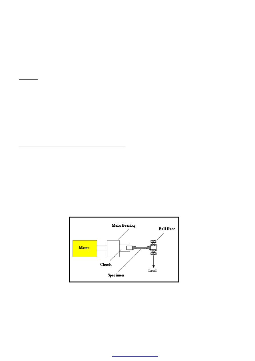
124
FATIGUE, CREEP AND FRACTURE
Fatigue
Fracture of components due to fatigue is the most common cause of service failure,
particularly in shafts, axles, aircraft wings, etc., where cyclic stressing is taking place.
With static loading of a ductile material, plastic flow precedes final fracture, the
specimen necks and the fractured surface reveals a fibrous structure, but with fatigue, the
crack is initiated from points of high stress concentration on the surface of the component
such as sharp changes in cross-section, slag inclusions, tool marks, etc., and then spreads
or propagates under the influence of the load cycles until it reaches a critical size when
fast fracture of the remaining cross-section takes place.
The Stress to number of cycles (S/N) curve
Fatigue tests are usually carried out under conditions of rotating - bending and with a
zero mean stress as obtained by means of a Wohler machine. From Figure (1), it
can be seen that the top surface of the specimen, held “cantilever fashion” in the machine,
is in tension, whilst the bottom surface is in compression. As the specimen rotates, the top
surface moves to the bottom and hence each segment of the surface moves continuously
from tension to compression producing a stress-cycle curve as shown in Figure (2). In
order to understand certain terms in common usage, let us consider a stress-cycle curve
where there is a positive tensile mean stress as may be obtained using other types of
fatigue machines such as a Haigh “push-pull” machine.
Figure (1) Single point load arrangement in a Wohler machine
for zero mean stress fatigue testing
PDF created with pdfFactory Pro trial version
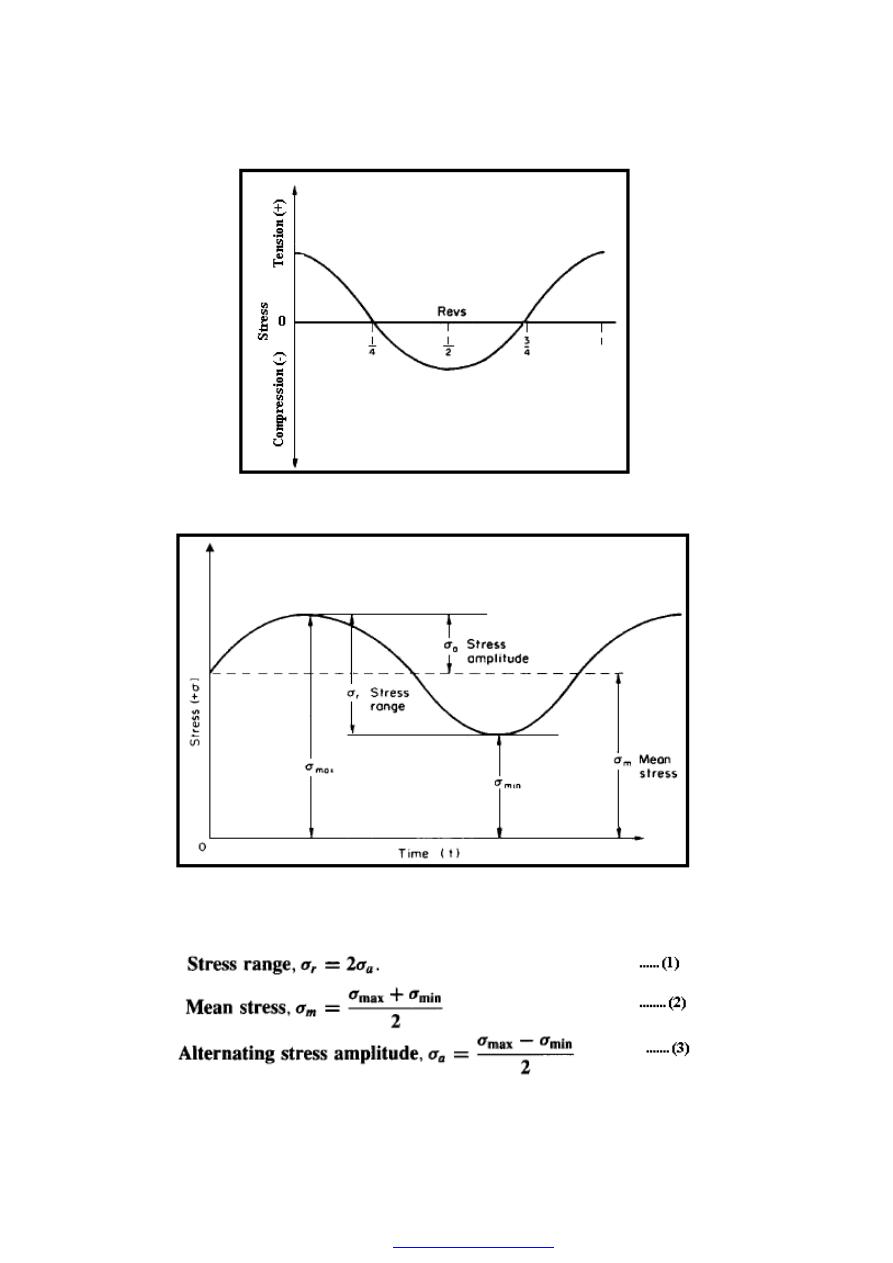
125
Figure (2) Simple sinusoidal (zero mean) stress fatigue
curve, “reversed-symmetrical”
Figure (3) Fluctuating tension stress cycle producing positive mean stress
The stress-cycle curve is shown in Figure (3), and from this diagram it can be seen that:
PDF created with pdfFactory Pro trial version
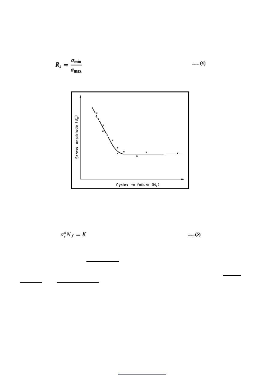
126
If the mean stress is not zero, we sometimes make use of the “stress ratio” R, where
The most general method of presenting the results of a fatigue test is to plot a graph of the
stress amplitude as ordinate against the corresponding number of cycles to failure.
Figure (4) Typical S/N curve fatigue life curve
In using the S/N curve for design purposes it may be advantageous to express the
relationship between (a) and (N
f
), the number of cycles to failure.
Where: (a) is a constant which varies from 8 to 15 and (K) is a second constant
depending on the material. From the S/N curve the “fatigue limit” or “endurance limit”
may be ascertained. The “fatigue limit” is the stress condition below which a material
may endure an infinite number of cycles prior to failure. Ferrous metal specimens often
produce S/N curves which exhibit fatigue limits as indicated in Figure (5a) The ‘fatigue
strength” or “endurance limit”, is the stress condition under which a specimen would
have a fatigue life of N cycles as shown in Figure (5B) Non-ferrous metal
specimens show this type of curve and hence components made from aluminium, copper
and nickel, etc., must always be designed for a finite life.
PDF created with pdfFactory Pro trial version
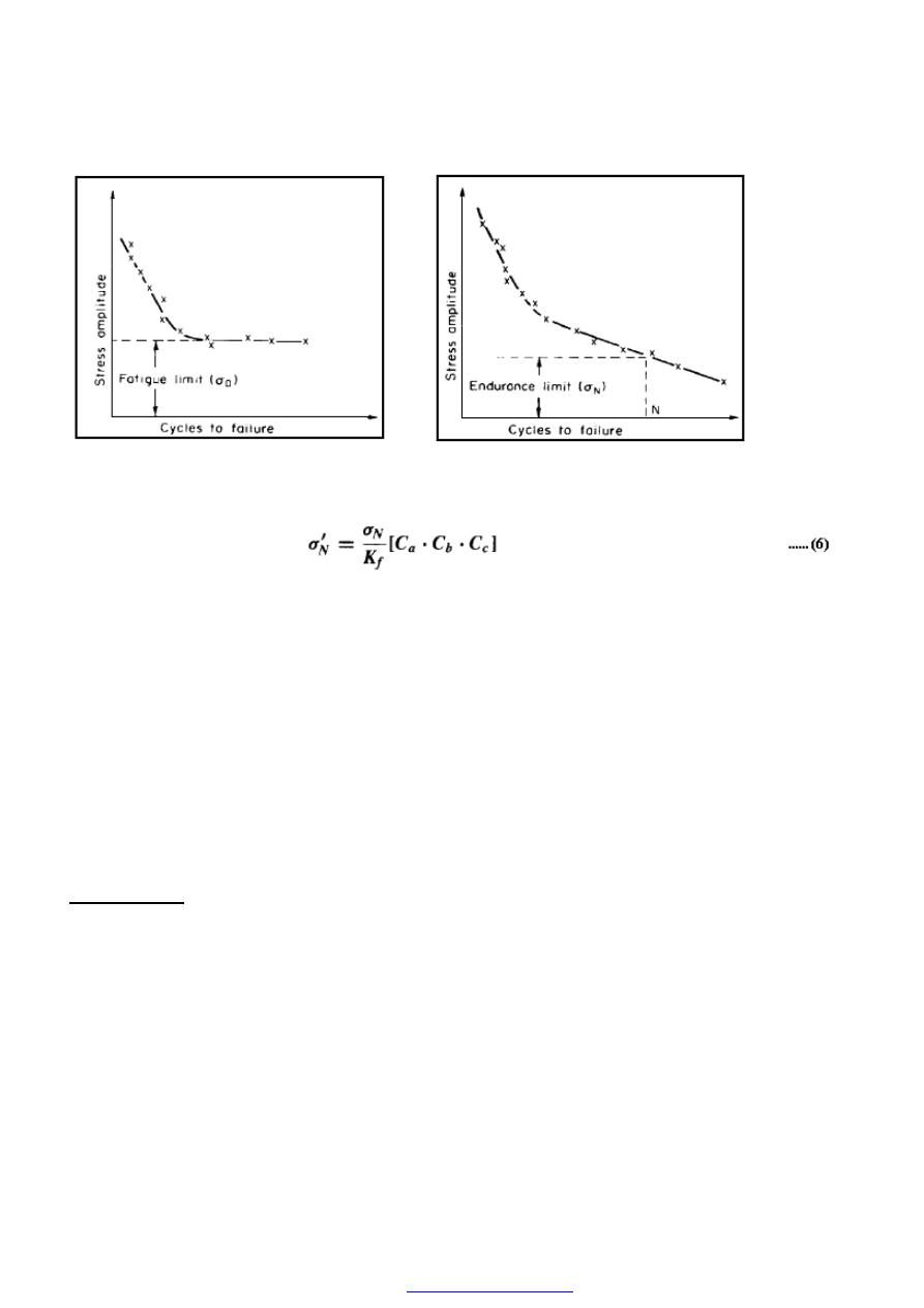
127
Figure (5) S/N curve showing (a) fatigue limit (b) endurance limit
Where (
N
σ
) oh is the “modified fatigue strength” or “modified fatigue limit”, (
N
σ
)is the
intrinsic value, (K
f
)is the fatigue strength reduction factor and C
a
, C
b
and C
c
are factors
allowing for size, surface finish, type of loading, etc.
The types of fatigue loading in common usage include direct stress, where the material
is repeatedly loaded in its axial direction; plane bending, where the material is bent about
its neutral plane; rotating bending, where the specimen is being rotated and at the same
time subjected to a bending moment; torsion, where the specimen is subjected to
conditions which produce reversed or fluctuating torsional stresses and, finally, combined
stress conditions, where two or more of the previous types of loading are operating
simultaneously.
P/S/N curves
The fatigue life of a component as determined at a particular stress level is a very
variable quantity so that seemingly identical specimens may give widely differing results.
This scatter arises from many sources including variations in material composition and
heterogeneity, variations in surface finish, variations in axiality of loading, etc.
PDF created with pdfFactory Pro trial version
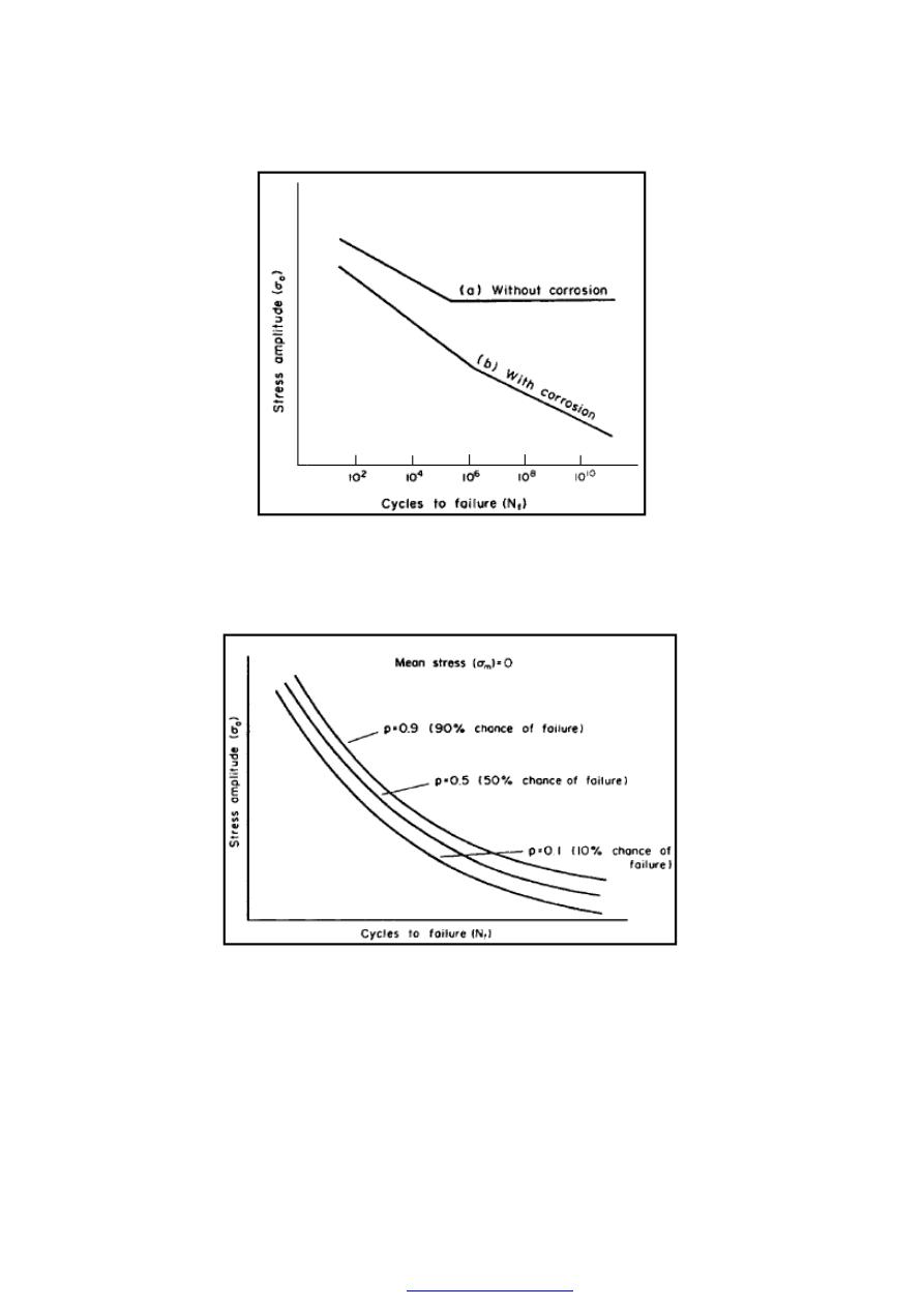
128
Figure (6) The effect of corrosion on fatigue life. S/N Curve for
(a) material showing fatigue limit; (b) same material under corrosion conditions
.
Figure (7) P/S/N curves indicating percentage chance of failure for given
stress level after known number of cycles(zero mean stress)
To overcome this problem, a number of test pieces should be tested at several different
stresses and then an estimate of the life at a particular stress level for a given probability
can be made.
PDF created with pdfFactory Pro trial version
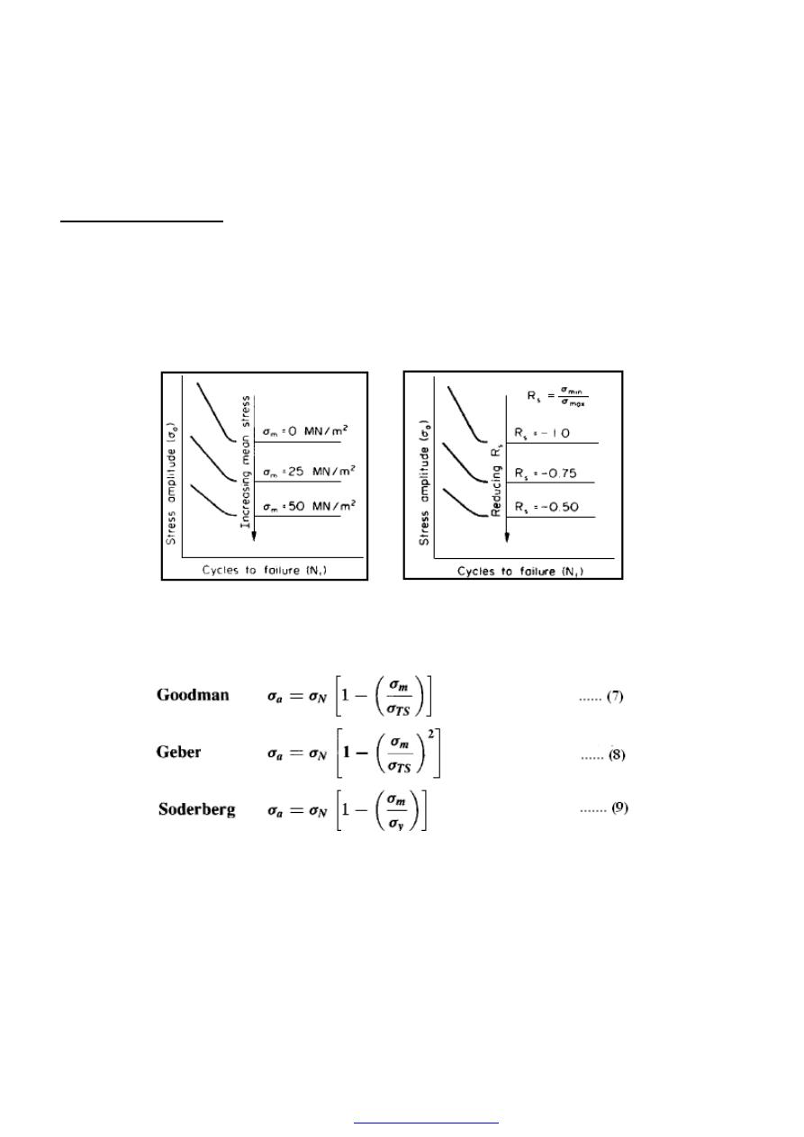
129
Effect of mean stress
If the fatigue test is carried out under conditions such that the mean stress is tensile
Figure (3), then, in order that the specimen will fail in the same number of cycles as a
similar specimen tested under zero mean stress conditions, the stress amplitude in the
former case will have to be reduced. The fact that an increasing tensile mean stress
lowers the fatigue or endurance limit is important, and all S/N curves should contain
information regarding the test conditions Figure (8).
Figure (8) Effect of mean stress on the S/N curve expressed in alternative ways
A number of investigations have been made of the quantitative effect of tensile mean
stress resulting in the following equations:
Where;
σ
Ν
= the fatigue strength for N cycles under zero mean stress conditions.
σ
a
= the fatigue strength for N cycles under condition of mean stress a,.
σ
TS
= tensile strength of the material.
σ
y
= yield strength of the material.
PDF created with pdfFactory Pro trial version
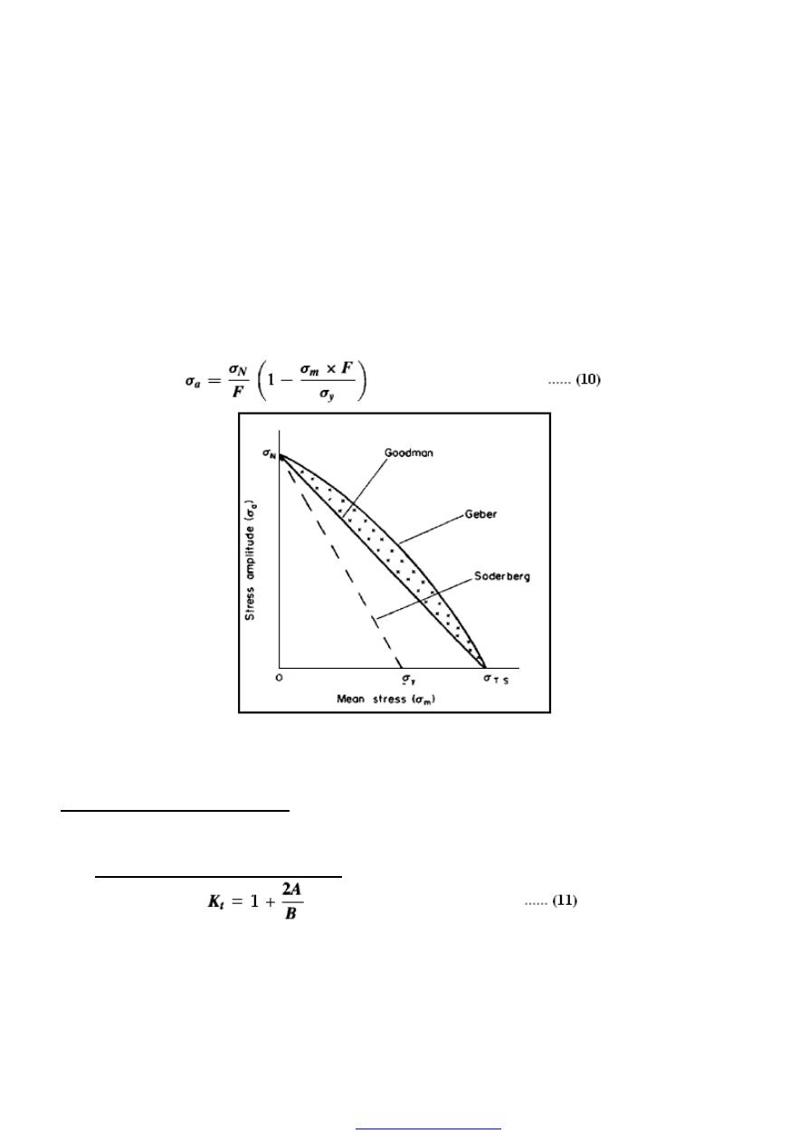
130
The above equations may be shown in graphical form Figure (9) and in actual practice it
has been found that most test results fall within the envelope formed by the parabolic
curve of Geber and the straight line of Goodman. However, because the use of Soderberg
gives an additional margin of safety, this is the equation often preferred .
Even when using the Soderberg equation it is usual to apply a factor of safety
(F) to both the alternating and the steady component of stress, in which case
equation (9) becomes:
Figure (9) Amplitude/mean stress relationships as per Goodman.
Geber and Soderberg
Effect of stress concentration
The influence of stress concentration can be illustrated by consideration of an
elliptical crack in a plate subjected to a tensile stress. Provided that the plate is very large,
the “theoretical stress concentration” factor (K
t
) is given by:
Where; “A” and
“B’ are the crack dimensions as shown in Figure (10). If the crack is
perpendicular to the direction of stress, then A is large compared with B and hence (K
t
)
PDF created with pdfFactory Pro trial version
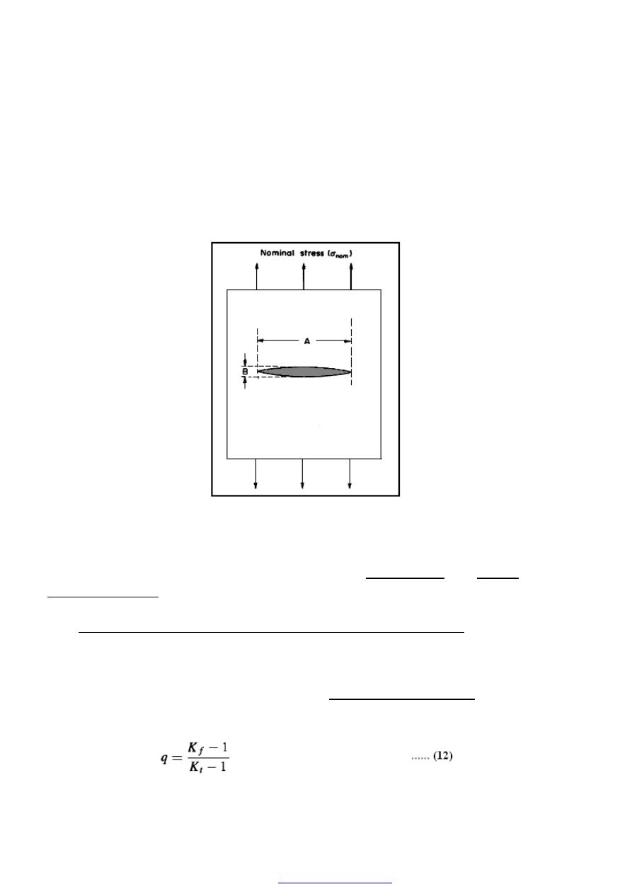
131
will be large. If the crack is parallel to the direction of stress, then A is very small
compared with B and hence K
t
= 1. If the dimensions of A and B are equal such that the
crack becomes a round hole, then K
t
= 3 and a maximum stress of (3
σ
nom.
), acts at the
sides of the hole.
Figure (10) Elliptical crack in semi-infinite plate
The effect of sudden changes of section, notches or defects upon the fatigue
performance of a component may be indicated by the “fatigue notch” or “fatigue
strength reduction” factor (K
f
) which is the ratio of the stress amplitude at the fatigue
limit of an un-notched specimen.
(K
f
) is always less than the static theoretical stress concentration factor referred to above
because under the compressive part of a tensile-compressive fatigue cycle, a
fatigue crack is unlikely to grow.
The extent to which the stress concentration effect under fatigue conditions approaches
that for static conditions is given by the “notch sensitivity factor” (q), and the
relationship between them may be simply expressed by:
PDF created with pdfFactory Pro trial version
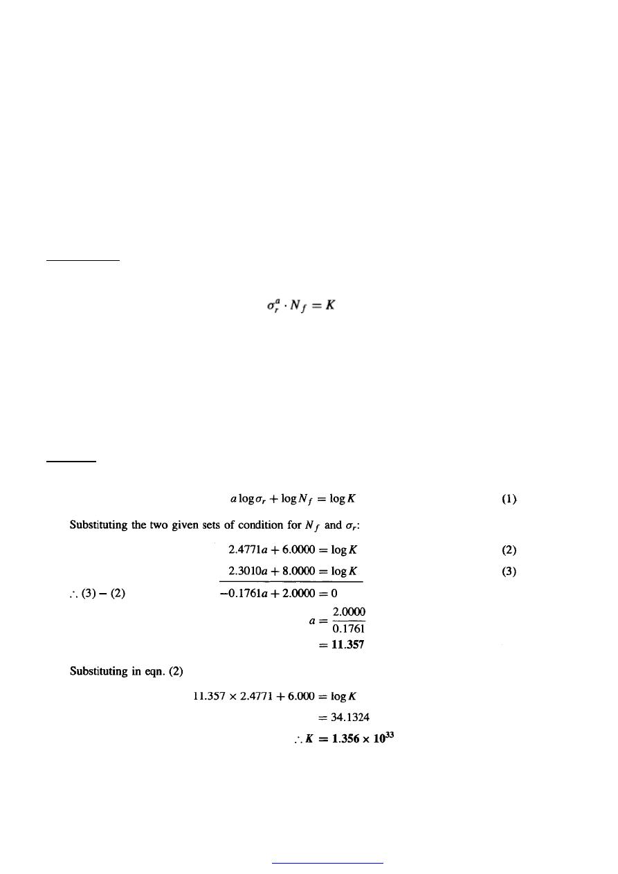
132
thus q is always less than 1.
Notch sensitivity is a very complex factor depending not only upon the material but
also upon the grain size, a finer grain size resulting in a higher value of q than a coarse
grain size.
Examples
Example (1)
The fatigue behavior of a specimen under alternating stress conditions with zero mean
stress is given by the expression:
Where;
σ
r
is the range of cyclic stress, N
f
is the number of cycles to failure and (K)
and (a) are material constants.
It is known that N
f
= l0
6
when,
σ
r
= 300 MN/m
2
and N
f
= 10
8
when
σ
r
= 200 MN/m
2
.
Calculate the constants (K) and (a) and hence the life of the specimen when subjected to
a stress range of 100 MN/m
2
.
Solution
Taking logarithms of the given expression we have:
PDF created with pdfFactory Pro trial version
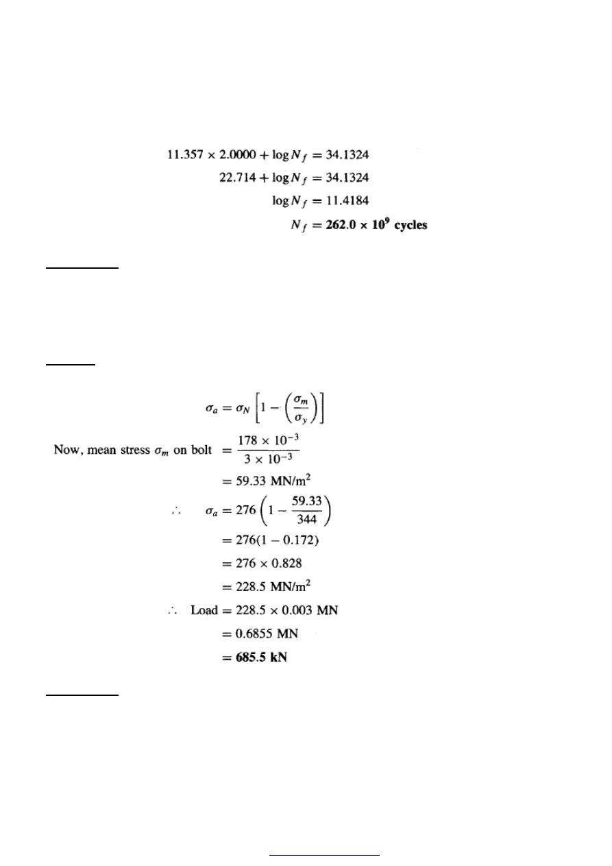
133
Hence, for stress range of 100 MN/m
2
, from equation (1);
Example (2)
A steel bolt 0.003 m
2
in cross-section is subjected to a static mean load of
178 kN. What value of completely reversed direct fatigue load will produce failure in l0
7
cycles? Use the Soderberg relationship and assume that the yield strength of the steel is
344 MN/m
2
and the stress required to produce failure at l0
7
cycles under zero mean stress
conditions is 276 MN/m
2
.
Solution
From equation of Soderberg
Example (3)
A stepped steel rod, the smaller section of which is 50 mm in diameter, is subjected to a
fluctuating direct axial load which varies from +178 kN to -178 kN. If the theoretical
stress concentration due to the reduction in section is 2.2, the notch sensitivity factor is
PDF created with pdfFactory Pro trial version
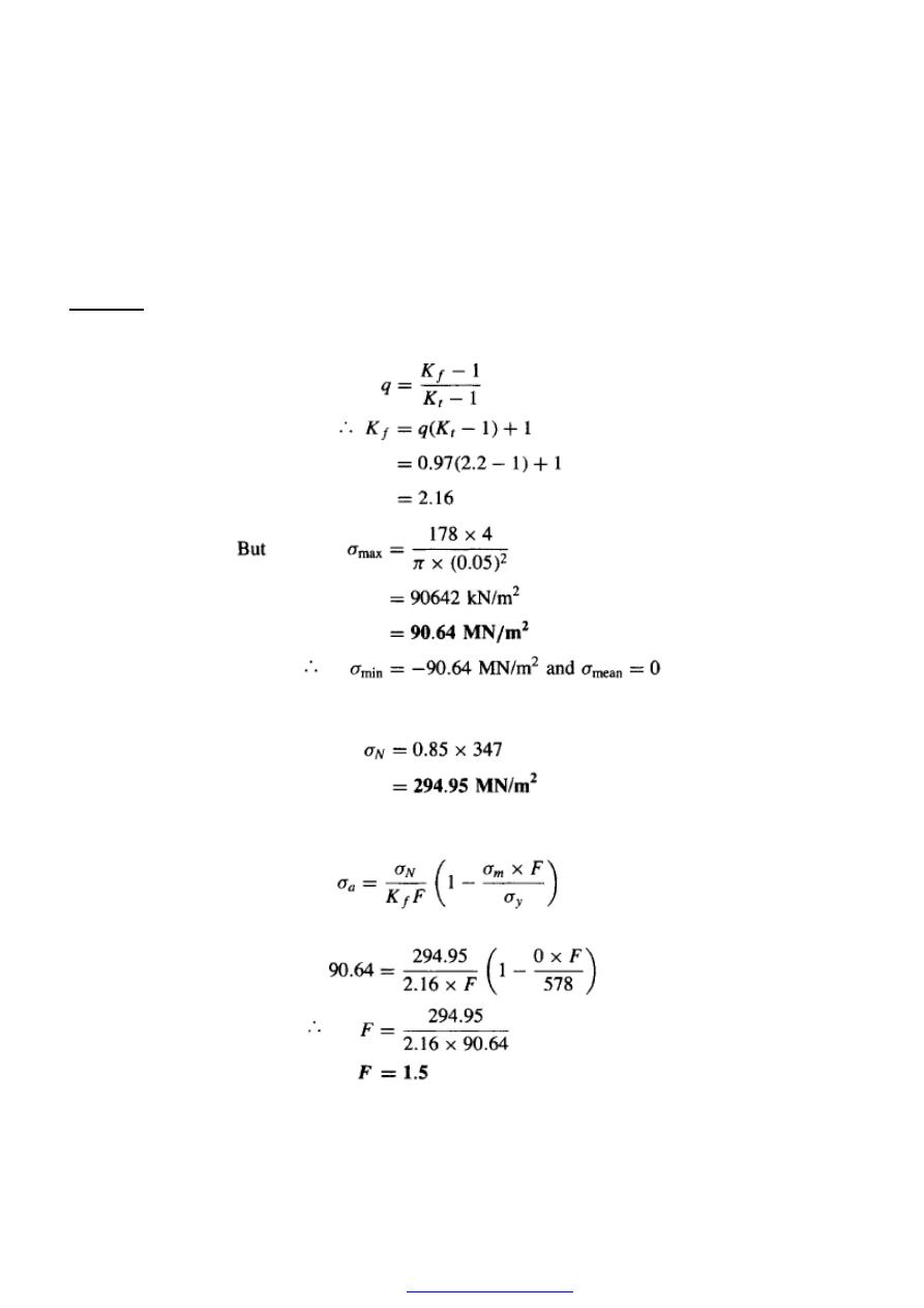
134
0.97, the yield strength of the material is 578 MN/m
2
and the fatigue limit under rotating
bending is 347 MN/m
2
, calculated the factor of safety if the fatigue limit in tension-
compression is 0.85 of that in rotating bending.
Solution
From equation (12)
:. Under direct stress conditions
From equation (13)
:. With common units of MN/m
2
:
PDF created with pdfFactory Pro trial version

135
Creep
Creep is the time-dependent deformation which accompanies the application of
stress to a material. At room temperatures, apart from the low-melting-point metals such
as lead, most metallic materials show only very small creep rates which can be ignored.
With increase in temperature, however, the creep rate also increases and above
approximately 0.4 T
m
where T
m
, is the melting point on the Kelvin scale, creep becomes
very significant.
The creep test
The creep test is usually carried out at a constant temperature and under constant
load conditions rather than at constant stress conditions. This is acceptable because it is
more representative of service conditions. A typical creep testing machine is shown in
Figure (1) Each end of the specimen is screwed into the specimen holder which is made
of a creep resisting alloy and thermocouples and accurate extensometers are fixed to the
specimen in order to measure temperature and strain. The electric furnace is then lowered
into place and when all is ready and the specimen is at the desired temperature, the load is
applied by adding weights to the lower arm and readings are taken at periodic intervals of
extension against time. It is important that accurate control of temperature is possible and
to facilitate this the equipment is often housed in a temperature-controlled room. The
results from the creep test are plotted in graphical form to produce a typical curve as
shown in Figure (2) After the initial extension OA which is produced as soon as the test
load is applied, and which is not part of the creep process proper (but which nevertheless
should not be ignored), the curve can be divided into three stages. In the first or primary
stage AB, the movement of dislocations is very rapid, any barriers to movement caused
by work-hardening being overcome by the recovery processes, albeit at a decreasing rate
.
Thus the initial creep strain rate is high but it rapidly decreases to a constant value. In the
secondary stage BC, the work-hardening process of “dislocation pile-up” and
“entanglement” are balanced by the recovery processes of “dislocation climb” and
“cross-slip”, to give a straight-line relationship and the slope of the graph in this steady-
state portion of the curve is equal to the secondary creep rate. Since, generally, the
primary and tertiary stages occur quickly, it is the secondary creep rate which is of prime
importance to the design engineer. The third or tertiary stage CD coincides with the
formation of internal voids within the specimen and this leads to “necking”, causing the
stress to increase and rapid failure to result.
PDF created with pdfFactory Pro trial version
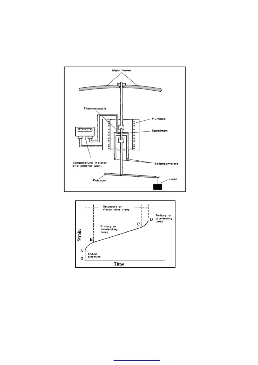
136
Figure (1) Schematic diagram of a typical creep testing machine
Figure (2) Typical creep curve
The shape of the creep curve for any material will depend upon the temperature of the
test and the stress at any time since these are the main factors controlling the work-
hardening and recovery processes. With increase in temperature, the creep rate increases
because the softening processes such as “dislocation climb” can take place more easily,
PDF created with pdfFactory Pro trial version
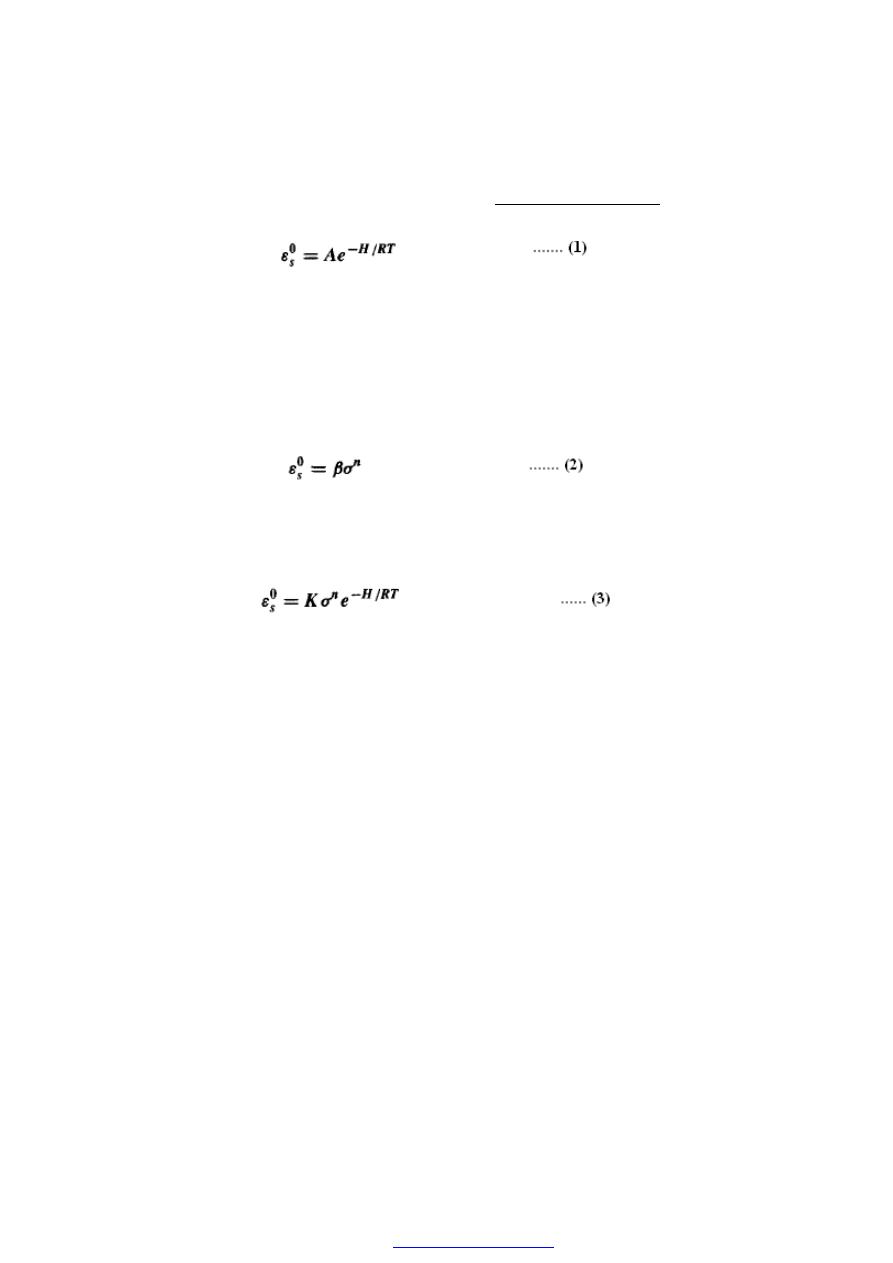
137
being diffusion controlled and hence a thermally activated process. It is expected,
therefore, that the creep rate is closely related to the Arrhenius equation,
viz.:
where (
0
s
ε ): is the secondary creep rate, H is the activation energy for creep for the
material under test, R is the universal gas constant, T is the absolute temperature and A is
a constant. It should be noted that both A and H are not true constants, their values
depending upon stress, temperature range and metallurgical variables.
The secondary creep rate also increases with increasing stress, the relationship being
most commonly expressed by the power law equation:
Where; (
β ) and (n) are constants, the value of n usually varying between 3 and 8.
Equations ( 1) and (2) may be combined to give:
Figure (3) illustrates the effect of increasing stress or temperature upon the creep curve
and it can be seen that increasing either of these two variables results in a similar change
of creep behavior, that is, an increase in the secondary or minimum creep rate, a
shortening of the secondary creep stage, and the earlier onset of tertiary creep and
fracture.
PDF created with pdfFactory Pro trial version
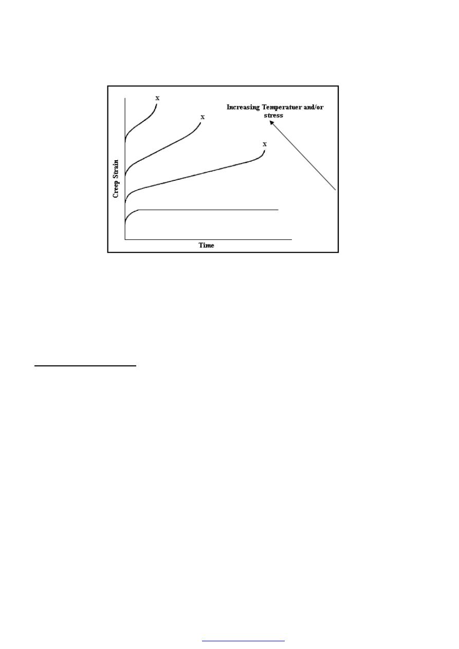
138
Figure (3) Creep curves showing effect of increasing temperature or stress
Fracture mechanics
The study of how materials fracture is known as fracture mechanics and the
resistance of a material to fracture is colloquially known as its “toughness”. No structure
is entirely free of defects and even on a microscopic scale these defects act as stress-
raisers which initiate the growth of cracks. The theory of fracture mechanics therefore
assumes the pre-existence of cracks and develops criteria for the catastrophic growth of
these cracks. In a stressed body, a crack can propagate in a combination of the three
opening modes shown in Figure (1) Mode I represents opening in a purely tensile field
while Modes II and III are in-plane and anti-plane shear modes respectively.
PDF created with pdfFactory Pro trial version
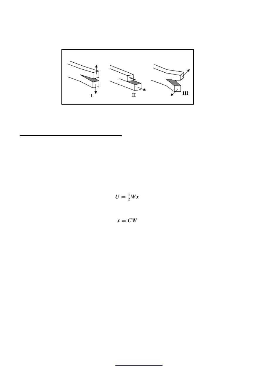
139
Figure (1) The three opening modes, associated with crack growth:
mode I-tensile; mode 11-in-plan
Energy variation in cracked bodies
It is assumed that a crack will only grow if there is a decrease in the free energy of
the system which comprises the cracked body and the loading mechanism. The first
usable criterion for fracture was developed from this assumption by Griffith(”).For a
clearer understanding of Griffith’s theory it is necessary to examine the changes in stored
elastic energy as a crack grows. Consider, therefore, the simple case of a strip containing
an edge crack of length (a) under uniaxial tension as shown in Figure (2) If load
(W) is applied gradually, the load points will move a distance (x) and the strain energy
(U) , stored in the body will be given by
for purely elastic deformation. The load and displacement are related by the
“compliance” C,
PDF created with pdfFactory Pro trial version
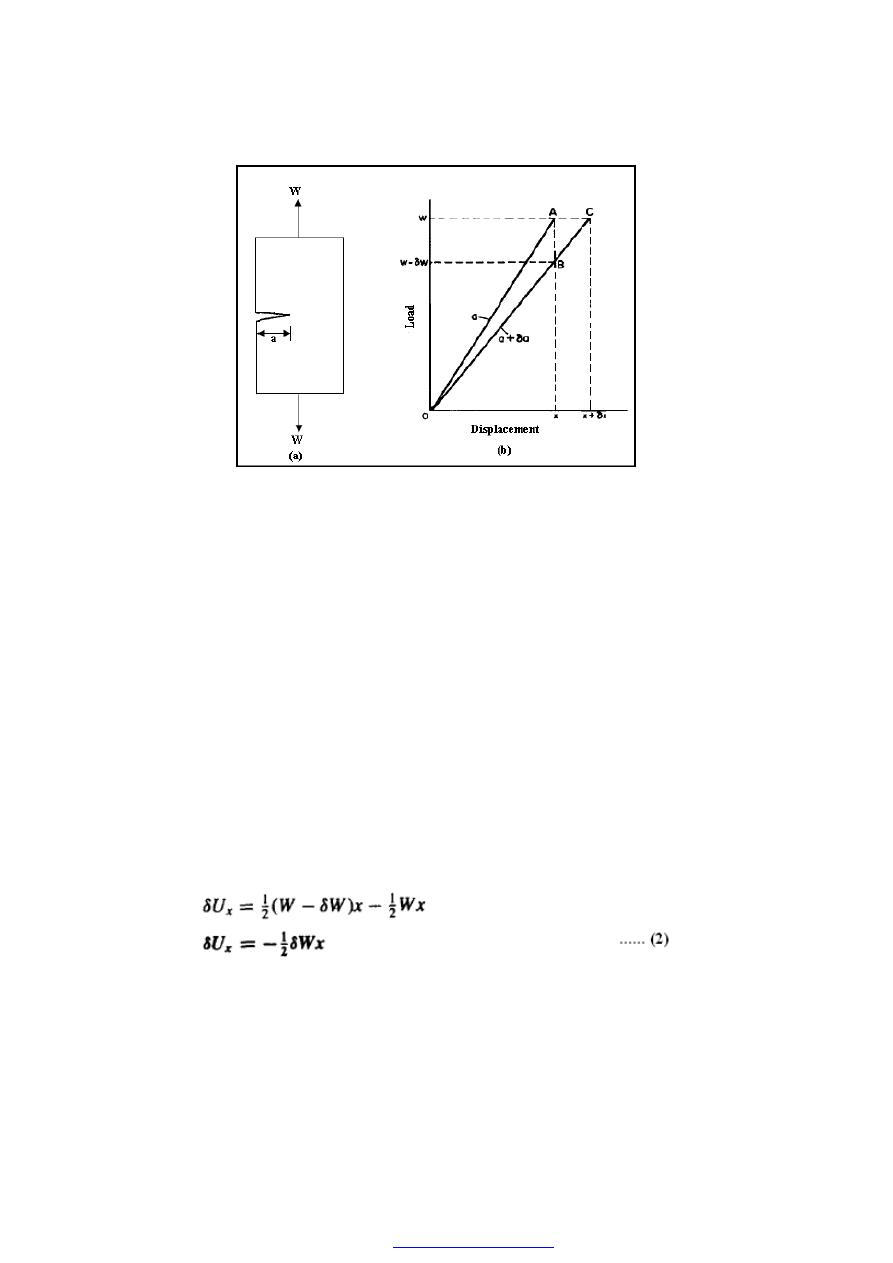
140
Figure (2) (a) Cracked body under tensile load W;
(b) force-displacement curves for a body with crack lengths a
and a + da.
The compliance is itself a function of the crack length but the exact relationship varies
with the geometry of the cracked body. However, if the crack length increases, the body
will become less stiff and the compliance will increase.
There are two limiting conditions to be considered depending on whether the cracked
body is maintained at (a) constant displacement or (b) constant loading. Generally a crack
will grow with both changing loads and displacement but these two conditions represent
the extreme constraints.
(a) Constant displacement
Consider the case shown in Figure (2)(b). If the body is taken to be perfectly elastic then
the load-displacement relationship will be linear. With an initial crack length (a) loading
will take place along the line OA. If the crack extends a small distance (
δ
a) while the
points of application of the load remain fixed, there will be a small increase in the
compliance resulting in a decrease in the load of (
δ
W). The load and displacement are
then given by the point B. The change in stored energy will then be given by
(b) Constant loading
In this case, if the crack again extends a small distance (
δ
a) the loading points must
move through an additional displacement (
δ
x) in order to keep the load
PDF created with pdfFactory Pro trial version
141
constant. The load and displacement are then represented by the point C. There would
appear to be an increase in stored energy given by
However, the load has supplied an amount of energy
This has to be obtained from external sources so that there is a total reduction in the
potential energy of the system of
For infinitesimally small increases in crack length the compliance C remains essentially
constant so that
Substituting in equation (3)
Comparison with equation (2) shows that, for small increases in crack length
,
It is therefore evident that for small increases in crack length there is a similar
decrease in potential energy no matter what the loading conditions. If there is a
decrease in potential energy when a crack grows then there must be an energy
requirement for the production of a crack - otherwise all cracked bodies would fracture
instantaneously.
Linear elastic fracture mechanics (L.E.F.M.)
(a) Griffrth’s criterion for fracture
Griffith’s thermodynamics approach was the first to produce a usable theory of
fracture mechanics. His theoretical model shown in Figure (3) was of an infinite sheet
under a remotely applied uniaxial stress (
σ
) and containing a central crack of length (2a).
Griffith, by a more mathematically rigorous treatment, was able to show that if that
decrease in energy is greater than the energy required to produce new crack faces then
there will be a net decrease in energy and the crack will propagate. For an increase in
crack length of (
δ
a).
PDF created with pdfFactory Pro trial version
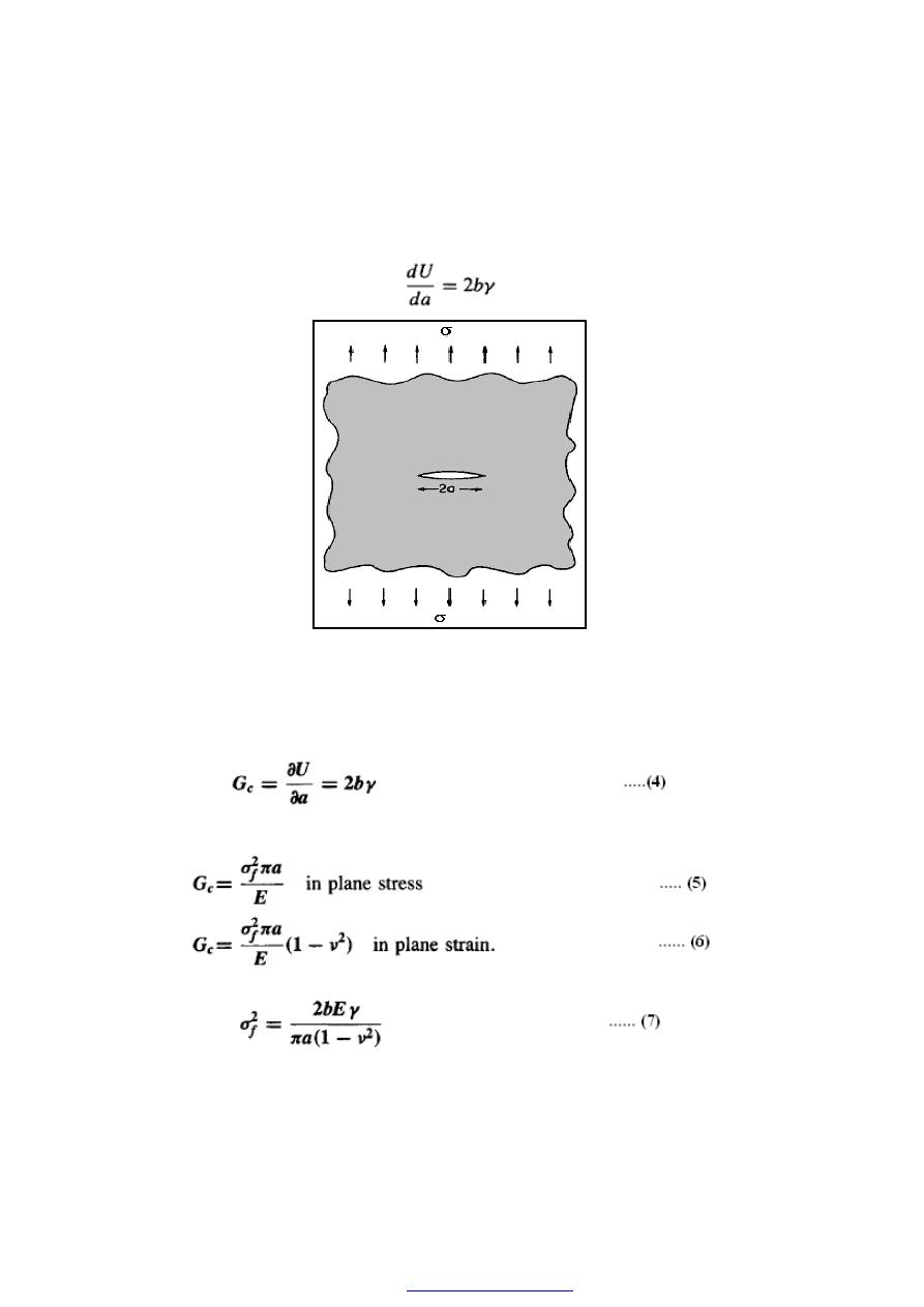
142
γ; is the surface energy of the crack faces;
b; is the thickness of the sheet.
At the onset of crack growth, (
δa) is small and we have
Figure (3) Mathematical model for Griffith’s analysis.
The expression on the left-hand side of the above equation is termed the
“critical strain
energy release
” (with respect to crack length) and is usually denoted as Gc,
This is the Griflth criterion for fracture.
Griffith’s analysis gives G, in terms of the fracture stress of
From equations (4) and (6) we can predict that, for plane strain, the fracture stress
or, for plane stress:
PDF created with pdfFactory Pro trial version
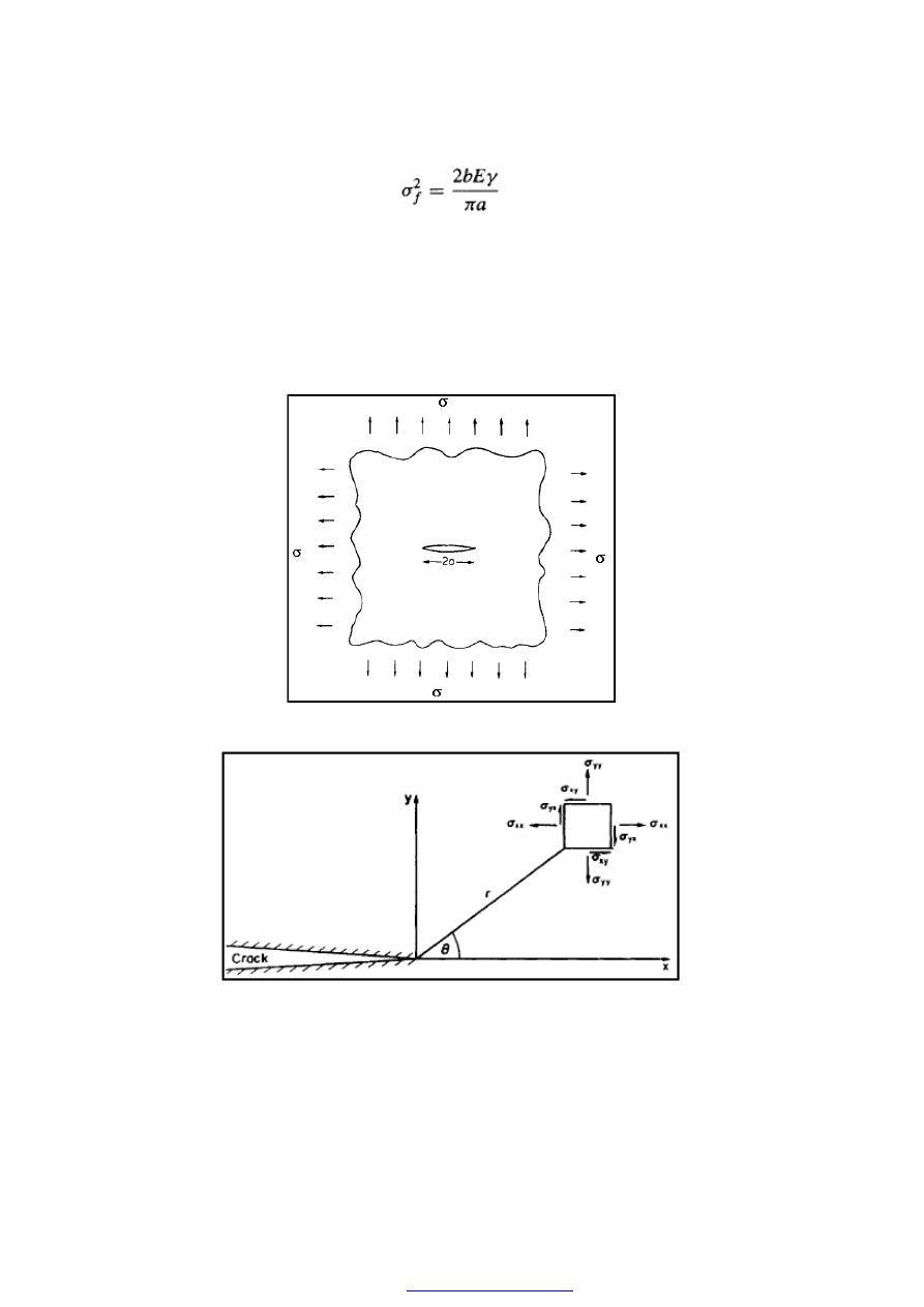
143
(b) Stress intensity factor
The elastic crack was developed by Irwin, who used a similar mathematical model
to that employed by Griffith except in this case the remotely applied stress is biaxial - see
Figure (4). Irwin's theory obtained expressions for the stress components near the crack
tip. The most elegant expression of the stress field is obtained by relating the Cartesian
components of stress to polar coordinates based at the crack tip as shown in Figure (5).
Figure (4) Mathematical model for Irwin's analysis
.
Figure (5) Coordinate system for stress components in Irwin's analysis.
Then we have:
PDF created with pdfFactory Pro trial version
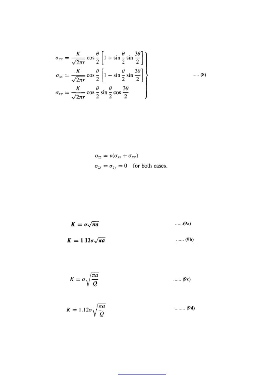
144
With, for plane stress
,
σ
zz
=0
or, for plane strain
,
If more than one crack opening mode is to be considered then K sometimes carries
the suffix I, II or III corresponding to the three modes shown in Figure (1). However
since this text is restricted to consideration of mode I crack propagation only, the
formulae have been simplified by adopting the symbol K without its suffix. K, in
development of similar formulae.
For Irwin’s model, K is given by
For an edge crack in a semi-infinite sheet
To accommodate different crack geometries a flaw shape parameter Q is sometimes
introduced thus
or, for an edge crack
PDF created with pdfFactory Pro trial version

145
Values of Q for various aspect (depth to width) ratios of crack can be obtained from
standard texts, but typically, they range from 1.0 for an aspect ratio of zero to 2.0 for an
aspect ratio of 0.4.
PDF created with pdfFactory Pro trial version