

i
About the Tutorial
MATLAB is a programming language developed by MathWorks. It started out as a
matrix programming language where linear algebra programming was simple. It
can be run both under interactive sessions and as a batch job.
This tutorial gives you aggressively a gentle introduction of MATLAB programming
language. It is designed to give students fluency in MATLAB programming
language. Problem-based MATLAB examples have been given in simple and easy
way to make your learning fast and effective.
Audience
This tutorial has been prepared for the beginners to help them understand basic
to advanced functionality of MATLAB. After completing this tutorial you will find
yourself at a moderate level of expertise in using MATLAB from where you can
take yourself to next levels.
Prerequisites
We assume you have a little knowledge of any computer programming and
understand concepts like variables, constants, expressions, statements, etc. If you
have done programming in any other high-level language like C, C++ or Java,
then it will be very much beneficial and learning MATLAB will be like a fun for you.
Copyright & Disclaimer Notice
Copyright 2014 by Tutorials Point (I) Pvt. Ltd.
All the content and graphics published in this e-book are the property of Tutorials Point (I)
Pvt. Ltd. The user of this e-book is prohibited to reuse, retain, copy, distribute or republish
any contents or a part of contents of this e-book in any manner without written consent
of the publisher.
We strive to update the contents of our website and tutorials as timely and as precisely as
possible, however, the contents may contain inaccuracies or errors. Tutorials Point
(I)
Pvt.
Ltd. provides no guarantee regarding the accuracy, timeliness or completeness of our
website or its contents including this tutorial. If you discover any errors on our website or
in this tutorial, please notify us at

ii
Table of Contents

iii

iv

v

vi

vii

viii

1
MATLAB (matrix laboratory) is a fourth-generation high-level programming
language and interactive environment for numerical computation, visualization
and programming.
MATLAB is developed by MathWorks.
It allows matrix manipulations; plotting of functions and data; implementation of
algorithms; creation of user interfaces; interfacing with programs written in other
languages, including C, C++, Java, and FORTRAN; analyze data; develop
algorithms; and create models and applications.
It has numerous built-in commands and math functions that help you in
mathematical calculations, generating plots, and performing numerical methods.
MATLAB's Power of Computational Mathematics
MATLAB is used in every facet of computational mathematics. Following are some
commonly used mathematical calculations where it is used most commonly:
Dealing with Matrices and Arrays
2-D and 3-D Plotting and graphics
Linear Algebra
Algebraic Equations
Non-linear Functions
Statistics
Data Analysis
Calculus and Differential Equations
Numerical Calculations
Integration
Transforms
Curve Fitting
Various other special functions
Features of MATLAB
Following are the basic features of MATLAB:
1.
OVERVIEW

2
It is a high-level language for numerical computation, visualization and
application development.
It also provides an interactive environment for iterative exploration, design
and problem solving.
It provides vast library of mathematical functions for linear algebra,
statistics, Fourier analysis, filtering, optimization, numerical integration and
solving ordinary differential equations.
It provides built-in graphics for visualizing data and tools for creating
custom plots.
MATLAB's programming interface gives development tools for improving
code quality, maintainability, and maximizing performance.
It provides tools for building applications with custom graphical interfaces.
It provides functions for integrating MATLAB based algorithms with external
applications and languages such as C, Java, .NET and Microsoft Excel.
Uses of MATLAB
MATLAB is widely used as a computational tool in science and engineering
encompassing the fields of physics, chemistry, math and all engineering streams.
It is used in a range of applications including:
signal processing and Communications
image and video Processing
control systems
test and measurement
computational finance
computational biology

3
Local Environment Setup
Setting up MATLAB environment is a matter of few clicks. The installer can be
downloaded from
http://in.mathworks.com/downloads/web_downloads
:
MathWorks provides the licensed product, a trial version and a student version as
well. You need to log into the site and wait a little for their approval.
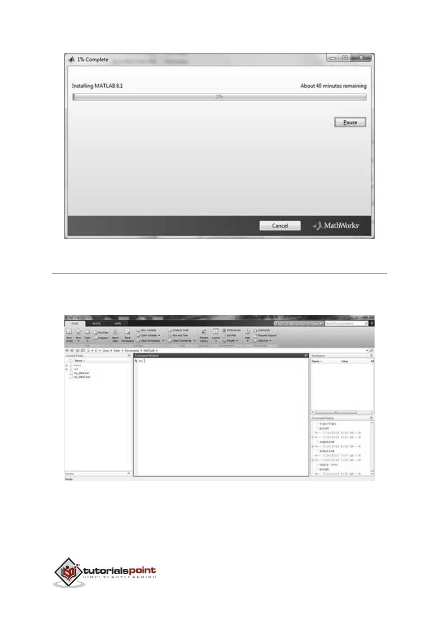
After downloading the installer the software can be installed through few clicks.
2.
ENVIRONMENT
4
Understanding the MATLAB Environment
MATLAB development IDE can be launched from the icon created on the desktop.
The main working window in MATLAB is called the desktop. When MATLAB is
started, the desktop appears in its default layout:
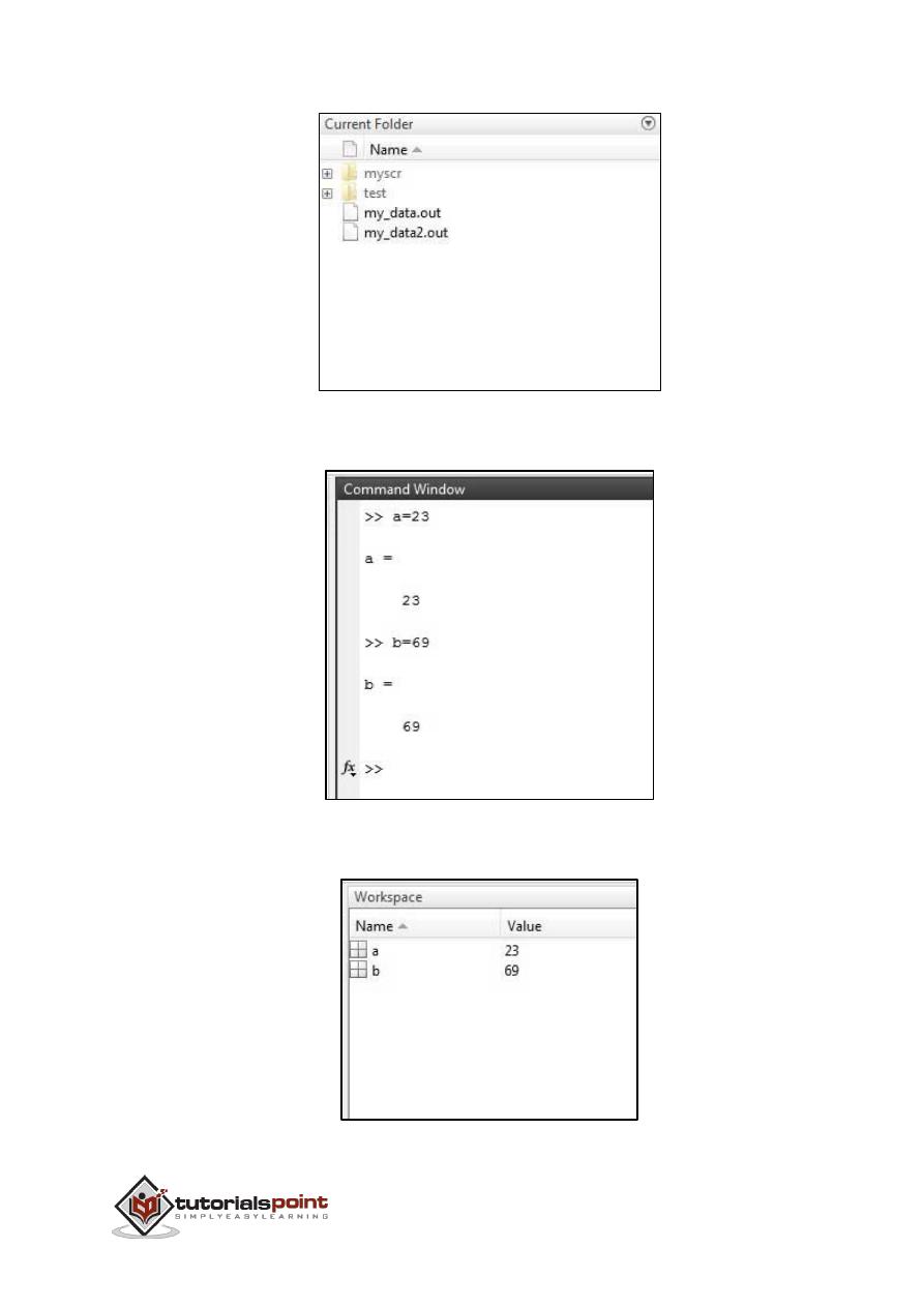
The desktop has the following panels:
Current Folder
- This panel allows you to access the project folders and files.
5
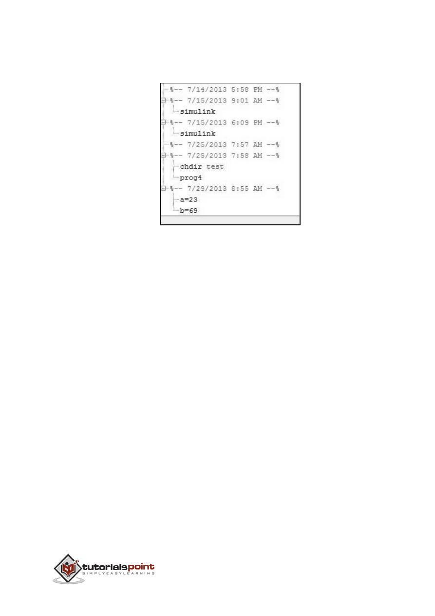
Command Window
- This is the main area where commands can be entered at
the command line. It is indicated by the command prompt (>>).
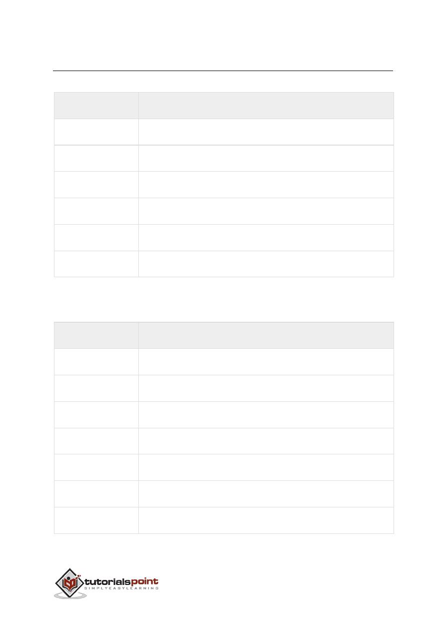
Workspace
- The workspace shows all the variables created and/or imported from
files.
6
Command History
- This panel shows or rerun commands that are entered at
the command line.
Set up GNU Octave
If you are willing to use Octave on your machine (Linux, BSD, OS X or Windows),
then
kindly
download
latest
version
from
http://www.gnu.org/software/octave/download.html
. You can check the given
installation instructions for your machine

7
MATLAB environment behaves like a super-complex calculator. You can enter
commands at the >> command prompt.
MATLAB is an interpreted environment. In other words, you give a command and
MATLAB executes it right away.
Hands on Practice
Type a valid expression, for example,
5
+
5
And press ENTER
When you click the Execute button, or type Ctrl+E, MATLAB executes it
immediately and the result returned is:
ans
=
10
Let us take up few more examples:
3
^
2
%
3
raised to the power of
2
When you click the Execute button, or type Ctrl+E, MATLAB executes it
immediately and the result returned is:
ans = 9
Another example,
sin
(
pi
/2)
%
sine of angle
90o
When you click the Execute button, or type Ctrl+E, MATLAB executes it
immediately and the result returned is:
ans = 1
3.
BASIC SYNTAX

8
Another example,
7/0
%
Divide
by
zero
When you click the Execute button, or type Ctrl+E, MATLAB executes it
immediately and the result returned is:
ans
=
Inf
warning
:
division
by
zero
Another example,
732
*
20.3
When you click the Execute button, or type Ctrl+E, MATLAB executes it
immediately and the result returned is:
ans
=
1.4860e+04
MATLAB provides some special expressions for some mathematical symbols, like
pi for π, Inf for ∞, i (and j) for √-1 etc.
Nan
stands for 'not a number'.
Use of Semicolon (;) in MATLAB
Semicolon (;) indicates end of statement. However, if you want to suppress and
hide the MATLAB output for an expression, add a semicolon after the expression.
For example,
x
=
3;
y
=
x
+
5
When you click the Execute button, or type Ctrl+E, MATLAB executes it
immediately and the result returned is:
y
=
8
Adding Comments
The percent symbol (%) is used for indicating a comment line. For example,

9
x
=
9
%
assign the value
9
to x
You can also write a block of comments using the block comment operators % {
and % }.
The MATLAB editor includes tools and context menu items to help you add,
remove, or change the format of comments.
Commonly used Operators and Special Characters
MATLAB supports the following commonly used operators and special characters:
Operator
Purpose
+
Plus; addition operator.
-
Minus; subtraction operator.
*
Scalar and matrix multiplication operator.
.*
Array multiplication operator.
^
Scalar and matrix exponentiation operator.
.^
Array exponentiation operator.
\
Left-division operator.
/
Right-division operator.
.\
Array left-division operator.
./
Array right-division operator.
:
Colon; generates regularly spaced elements and represents
an entire row or column.

10
( )
Parentheses; encloses function arguments and array
indices; overrides precedence.
[ ]
Brackets; enclosures array elements.
.
Decimal point.
…
Ellipsis; line-continuation operator
,
Comma; separates statements and elements in a row
;
Semicolon; separates columns and suppresses display.
%
Percent sign; designates a comment and specifies
formatting.
_
Quote sign and transpose operator.
._
Non-conjugated transpose operator.
=
Assignment operator.
Special Variables and Constants
MATLAB supports the following special variables and constants:
Name
Meaning
ans
Most recent answer.
eps
Accuracy of floating-point precision.
i,j
The imaginary unit √-1.
Inf
Infinity.

11
NaN
Undefined numerical result (not a number).
pi
The number π
Naming Variables
Variable names consist of a letter followed by any number of letters, digits or
underscore.
MATLAB is
case-sensitive.
Variable names can be of any length, however, MATLAB uses only first N
characters, where N is given by the function
namelengthmax.
Saving Your Work
The
save
command is used for saving all the variables in the workspace, as a file
with .mat extension, in the current directory.
For example,
save myfile
You can reload the file anytime later using the
load
command.
load myfile

12
In MATLAB environment, every variable is an array or matrix.
You can assign variables in a simple way. For example,
x
=
3
%
defining x
and
initializing it
with
a value
MATLAB will execute the above statement and return the following result:
x
=
3
It creates a 1-by-1 matrix named
x
and stores the value 3 in its element. Let us
check another example,
x
=
sqrt
(16)
%
defining x
and
initializing it
with
an expression
MATLAB will execute the above statement and return the following result:
x
=
4
Please note that:
Once a variable is entered into the system, you can refer to it later.
Variables must have values before they are used.
When an expression returns a result that is not assigned to any variable, the
system assigns it to a variable named ans, which can be used later.
For example,
sqrt
(78)
MATLAB will execute the above statement and return the following result:
ans
=
8.8318
4.
VARIABLES

13
You can use this variable
ans:
9876/
ans
MATLAB will execute the above statement and return the following result:
ans
=
1.1182e+03
Let's look at another example:
x
=
7
*
8;
y
=
x
*
7.89
MATLAB will execute the above statement and return the following result:
y
=
441.8400
Multiple Assignments
You can have multiple assignments on the same line. For example,
a
=
2;
b
=
7;
c
=
a
*
b;
MATLAB will execute the above statement and return the following result:
c =
14
I have forgotten the Variables!
The
who
command displays all the variable names you have used.
who
MATLAB will execute the above statement and return the following result:

14
Your
variables are
:
a ans b c x y
The
whos
command displays little more about the variables:
Variables currently in memory
Type of each variables
Memory allocated to each variable
Whether they are complex variables or not
whos
MATLAB will execute the above statement and return the following result:
Name Size Bytes Class Attributes
a 1x1 8 double
ans 1x1 8 double
b 1x1 8 double
c 1x1 8 double
x 1x1 8 double
y 1x1 8 double
The
clear
command deletes all (or the specified) variable(s) from the memory.
clear x % it will delete x, won't display anything
clear % it will delete all variables in the workspace
% peacefully and unobtrusively
Long Assignments
Long assignments can be extended to another line by using an ellipses (...). For
example,
initial_velocity = 0;
acceleration = 9.8;

15
time = 20;
final_velocity = initial_velocity ...
+ acceleration * time
MATLAB will execute the above statement and return the following result:
final_velocity =
196
The
format
Command
By default, MATLAB displays numbers with four decimal place values. This is
known as short format.
However, if you want more precision, you need to use the
format
command.
The
format long
command displays 16 digits after decimal.
For example:
format long
x = 7 + 10/3 + 5 ^ 1.2
MATLAB will execute the above statement and return the following result:
x =
17.231981640639408
Another example,
format
short
x
=
7
+
10/3
+
5
^
1.2
MATLAB will execute the above statement and return the following result:
x =
17.2320
The
format bank
command rounds numbers to two decimal places. For example,

16
format bank
daily_wage = 177.45;
weekly_wage = daily_wage * 6
MATLAB will execute the above statement and return the following result:
weekly_wage
=
1064.70
MATLAB displays large numbers using exponential notation.
The
format short e
command allows displaying in exponential form with four
decimal places plus the exponent.
For example,
format
short
e
4.678
*
4.9
MATLAB will execute the above statement and return the following result:
ans
=
2.2922e+01
The
format long e
command allows displaying in exponential form with four
decimal places plus the exponent. For example,
format
long
e
x
=
pi
MATLAB will execute the above statement and return the following result:
x
=
3.141592653589793e+00
The
format rat
command gives the closest rational expression resulting from a
calculation. For example,
format rat

17
4.678
*
4.9
MATLAB will execute the above statement and return the following result:
ans
=
2063/90
Creating Vectors
A vector is a one-dimensional array of numbers. MATLAB allows creating two types
of vectors:
Row vectors
Column vectors
Row vectors
are created by enclosing the set of elements in square brackets,
using space or comma to delimit the elements.
For example,
r
=
[7
8
9
10
11]
MATLAB will execute the above statement and return the following result:
r
=
Columns
1
through
4
7
8
9
10
Column
5
11
Another example,
r
=
[7
8
9
10
11];
t
=
[2,
3,
4,
5,
6];
res
=
r
+
t
MATLAB will execute the above statement and return the following result:

18
res
=
Columns
1
through
4
9
11
13
15
Column
5
17
Column vectors
are created by enclosing the set of elements in square brackets,
using semicolon (;) to delimit the elements.
c
=
[7;
8;
9;
10;
11]
MATLAB will execute the above statement and return the following result:
c
=
7
8
9
10
11
Creating Matrices
A matrix is a two-dimensional array of numbers.
In MATLAB, a matrix is created by entering each row as a sequence of space or
comma separated elements, and end of a row is demarcated by a semicolon. For
example, let us create a 3-by-3 matrix as:
m
=
[1
2
3;
4
5
6;
7
8
9]
MATLAB will execute the above statement and return the following result:
m
=
1
2
3
4
5
6

19
7
8
9

20
MATLAB is an interactive program for numerical computation and data
visualization. You can enter a command by typing it at the MATLAB prompt '>>'
on the
Command Window.
In this section, we will provide lists of commonly used general MATLAB commands.
Commands for Managing a Session
MATLAB provides various commands for managing a session. The following table
provides all such commands:
Command
Purpose
clc
Clears command window.
clear
Removes variables from memory.
exist
Checks for existence of file or variable.
global
Declares variables to be global.
help
Searches for a help topic.
lookfor
Searches help entries for a keyword.
quit
Stops MATLAB.
who
Lists current variables.
whos
Lists current variables (long display).
Commands for Working with the System
MATLAB provides various useful commands for working with the system, like
saving the current work in the workspace as a file and loading the file later.
5.
COMMANDS

21
It also provides various commands for other system-related activities like,
displaying date, listing files in the directory, displaying current directory, etc.
The following table displays some commonly used system-related commands:
Command
Purpose
cd
Changes current directory.
date
Displays current date.
delete
Deletes a file.
diary
Switches on/off diary file recording.
dir
Lists all files in current directory.
load
Loads workspace variables from a file.
path
Displays search path.
pwd
Displays current directory.
save
Saves workspace variables in a file.
type
Displays contents of a file.
what
Lists all MATLAB files in the current directory.
wklread
Reads .wk1 spreadsheet file.
22
Input and Output Commands
MATLAB provides the following input and output related commands:
Command
Purpose
disp
Displays contents of an array or string.
fscanf
Read formatted data from a file.
format
Controls screen-display format.
fprintf
Performs formatted writes to screen or file.
input
Displays prompts and waits for input.
;
Suppresses screen printing.
The
fscanf
and
fprintf
commands behave like C scanf and printf functions. They
support the following format codes:
Format Code
Purpose
%s
Format as a string.
%d
Format as an integer.
%f
Format as a floating point value.
%e
Format as a floating point value in scientific notation.
%g
Format in the most compact form: %f or %e.
\n
Insert a new line in the output string.
\t
Insert a tab in the output string.

23
The format function has the following forms used for numeric display:
Format Function Display up to
format short
Four decimal digits (default).
format long
16 decimal digits.
format short e
Five digits plus exponent.
format long e
16 digits plus exponents.
format bank
Two decimal digits.
format +
Positive, negative, or zero.
format rat
Rational approximation.
format compact Suppresses some line feeds.
format loose
Resets to less compact display mode.
Vector, Matrix, and Array Commands
The following table shows various commands used for working with arrays,
matrices and vectors:
Command
Purpose
cat
Concatenates arrays.
find
Finds indices of nonzero elements.
length
Computes number of elements.
linspace
Creates regularly spaced vector.

24
logspace
Creates logarithmically spaced vector.
max
Returns largest element.
min
Returns smallest element.
prod
Product of each column.
reshape
Changes size.
size
Computes array size.
sort
Sorts each column.
sum
Sums each column.
eye
Creates an identity matrix.
ones
Creates an array of ones.
zeros
Creates an array of zeros.
cross
Computes matrix cross products.
dot
Computes matrix dot products.
det
Computes determinant of an array.
inv
Computes inverse of a matrix.
pinv
Computes pseudoinverse of a matrix.
rank
Computes rank of a matrix.
rref
Computes reduced row echelon form.
25
cell
Creates cell array.
celldisp
Displays cell array.
cellplot
Displays graphical representation of cell array.
num2cell
Converts numeric array to cell array.
deal
Matches input and output lists.
iscell
Identifies cell array.
Plotting Commands
MATLAB provides numerous commands for plotting graphs. The following table
shows some of the commonly used commands for plotting:
Command
Purpose
axis
Sets axis limits.
fplot
Intelligent plotting of functions.
grid
Displays gridlines.
plot
Generates xy plot.
Prints plot or saves plot to a file.
title
Puts text at top of plot.
xlabel
Adds text label to x-axis.
ylabel
Adds text label to y-axis.
axes
Creates axes objects.

26
close
Closes the current plot.
close all
Closes all plots.
figure
Opens a new figure window.
gtext
Enables label placement by mouse.
hold
Freezes current plot.
legend
Legend placement by mouse.
refresh
Redraws current figure window.
set
Specifies properties of objects such as axes.
subplot
Creates plots in sub windows.
text
Places string in figure.
bar
Creates bar chart.
loglog
Creates log-log plot.
polar
Creates polar plot.
semilogx
Creates semi log plot. (logarithmic abscissa).
semilogy
Creates semi log plot. (logarithmic ordinate).
stairs
Creates stairs plot.
stem
Creates stem plot.

27
So far, we have used MATLAB environment as a calculator. However, MATLAB is
also a powerful programming language, as well as an interactive computational
environment.
In previous chapters, you have learned how to enter commands from the MATLAB
command prompt. MATLAB also allows you to write series of commands into a file
and execute the file as complete unit, like writing a function and calling it.
The M Files
MATLAB allows writing two kinds of program files:
Scripts
- script files are program files with
.m extension. In these files, you write
series of commands, which you want to execute together. Scripts do not accept
inputs and do not return any outputs. They operate on data in the workspace.
Functions
- functions files are also program files with
.m extension. Functions
can accept inputs and return outputs. Internal variables are local to the function.
You can use the MATLAB editor or any other text editor to create your
.m
files. In
this section, we will discuss the script files. A script file contains multiple sequential
lines of MATLAB commands and function calls. You can run a script by typing its
name at the command line.
Creating and Running Script File
To create scripts files, you need to use a text editor. You can open the MATLAB
editor in two ways:
Using the command prompt
Using the IDE
If you are using the command prompt, type
edit
in the command prompt. This
will open the editor. You can directly type
edit
and then the filename (with .m
extension)
edit
Or
edit
<filename>
6.
M-FILES
28
The above command will create the file in default MATLAB directory. If you want
to store all program files in a specific folder, then you will have to provide the
entire path.
Let us create a folder named progs. Type the following commands at the command
prompt(>>):
mkdir progs
%
create directory progs under
default
directory
chdir progs
%
changing the current directory to progs
edit prog1
.
m
%
creating an m file named prog1
.
m
If you are creating the file for first time, MATLAB prompts you to confirm it. Click
Yes.
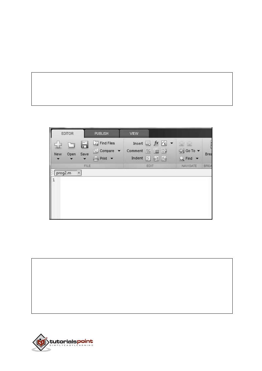
Alternatively, if you are using the IDE, choose NEW -> Script. This also opens the
editor and creates a file named Untitled. You can name and save the file after
typing the code.
Type the following code in the editor:
NoOfStudents
=
6000;
TeachingStaff
=
150;
NonTeachingStaff
=
20;
Total
=
NoOfStudents
+
TeachingStaff
...
+
NonTeachingStaff;

29
disp
(Total);
After creating and saving the file, you can run it in two ways:
Clicking the
Run
button on the editor window or
Just typing the filename (without extension) in the command prompt: >> prog1
The command window prompt displays the result:
6170
Example
Create a script file, and type the following code:
a
=
5;
b
=
7;
c
=
a
+
b
d
=
c
+
sin
(
b
)
e
=
5
*
d
f
=
exp
(-
d
)
When the above code is compiled and executed, it produces the following result:
c
=
12
d
=
12.6570
e
=
63.2849
f
=
3.1852e-06

30
MATLAB does not require any type declaration or dimension statements.
Whenever MATLAB encounters a new variable name, it creates the variable and
allocates appropriate memory space.
If the variable already exists, then MATLAB replaces the original content with new
content and allocates new storage space, where necessary.
For example,
Total
=
42
The above statement creates a 1-by-1 matrix named 'Total' and stores the value
42 in it.
Data Types Available in MATLAB
MATLAB provides 15 fundamental data types. Every data type stores data that is
in the form of a matrix or array. The size of this matrix or array is a minimum of
0-by-0 and this can grow up to a matrix or array of any size.
The following table shows the most commonly used data types in MATLAB:
Data Type
Description
int8
8-bit signed integer
uint8
8-bit unsigned integer
int16
16-bit signed integer
uint16
16-bit unsigned integer
int32
32-bit signed integer
uint32
32-bit unsigned integer
int64
64-bit signed integer
7.
DATA TYPES

31
uint64
64-bit unsigned integer
single
single precision numerical data
double
double precision numerical data
logical
logical values of 1 or 0, represent true and false respectively
char
character data (strings are stored as vector of characters)
cell array
array of indexed cells, each capable of storing an array of a
different dimension and data type
structure
C-like structures, each structure having named fields
capable of storing an array of a different dimension and data
type
function handle pointer to a function
user classes
objects constructed from a user-defined class
java classes
objects constructed from a Java class
Example
Create a script file with the following code:
str
=
'Hello World!'
n
=
2345
d
=
double(
n
)
un
=
uint32
(789.50)
rn
=
5678.92347
c
=
int32
(
rn
)

32
When the above code is compiled and executed, it produces the following result:
str
=
Hello
World!
n
=
2345
d
=
2345
un
=
790
rn
=
5.6789e+03
c
=
5679
Data Type Conversion
MATLAB provides various functions for converting a value from one data type to
another. The following table shows the data type conversion functions:
Function
Purpose
Char
Convert to character array (string)
int2str
Convert integer data to string
mat2str
Convert matrix to string
num2str
Convert number to string
str2double
Convert string to double-precision value

33
str2num
Convert string to number
native2unicode
Convert numeric bytes to Unicode characters
unicode2native
Convert Unicode characters to numeric bytes
base2dec
Convert base N number string to decimal number
bin2dec
Convert binary number string to decimal number
dec2base
Convert decimal to base N number in string
dec2bin
Convert decimal to binary number in string
dec2hex
Convert decimal to hexadecimal number in string
hex2dec
Convert hexadecimal number string to decimal number
hex2num
Convert hexadecimal number string to double-precision
number
num2hex
Convert singles and doubles to IEEE hexadecimal strings
cell2mat
Convert cell array to numeric array
cell2struct
Convert cell array to structure array
cellstr
Create cell array of strings from character array
mat2cell
Convert array to cell array with potentially different sized
cells
num2cell
Convert array to cell array with consistently sized cells
struct2cell
Convert structure to cell array

34
Determination of Data Types
MATLAB provides various functions for identifying data type of a variable.
Following table provides the functions for determining the data type of a variable:
Function
Purpose
is
Detect state
isa
Determine if input is object of specified class
iscell
Determine whether input is cell array
iscellstr
Determine whether input is cell array of strings
ischar
Determine whether item is character array
isfield
Determine whether input is structure array field
isfloat
Determine if input is floating-point array
ishghandle
True for Handle Graphics object handles
isinteger
Determine if input is integer array
isjava
Determine if input is Java object
islogical
Determine if input is logical array
isnumeric
Determine if input is numeric array
isobject
Determine if input is MATLAB object
isreal
Check if input is real array
isscalar
Determine whether input is scalar

35
isstr
Determine whether input is character array
isstruct
Determine whether input is structure array
isvector
Determine whether input is vector
class
Determine class of object
validateattributes Check validity of array
whos
List variables in workspace, with sizes and types
Example
Create a script file with the following code:
x
=
3
isinteger
(
x
)
isfloat
(
x
)
isvector
(
x
)
isscalar
(
x
)
isnumeric
(
x
)
x
=
23.54
isinteger
(
x
)
isfloat
(
x
)
isvector
(
x
)
isscalar
(
x
)
isnumeric
(
x
)
x
=
[1
2
3]

36
isinteger
(
x
)
isfloat
(
x
)
isvector
(
x
)
isscalar
(
x
)
x
=
'Hello'
isinteger
(
x
)
isfloat
(
x
)
isvector
(
x
)
isscalar
(
x
)
isnumeric
(
x
)
When you run the file, it produces the following result:
x
=
3
ans
=
0
ans
=
1
ans
=
1
ans
=
1
ans
=
1
x
=
23.5400

37
ans
=
0
ans
=
1
ans
=
1
ans
=
1
ans
=
1
x
=
1
2
3
ans
=
0
ans
=
1
ans
=
1
ans
=
0
x
=
Hello
ans
=
0
ans
=
0

38
ans
=
1
ans
=
0
ans
=
0

39
An operator is a symbol that tells the compiler to perform specific mathematical
or logical manipulations. MATLAB is designed to operate primarily on whole
matrices and arrays. Therefore, operators in MATLAB work both on scalar and non-
scalar data. MATLAB allows the following types of elementary operations:
Arithmetic Operators
Relational Operators
Logical Operators
Bitwise Operations
Set Operations
Arithmetic Operators
MATLAB allows two different types of arithmetic operations:
Matrix arithmetic operations
Array arithmetic operations
Matrix arithmetic operations are same as defined in linear algebra. Array operations are executed
element by element, both on one-dimensional and multidimensional array.
The matrix operators and array operators are differentiated by the period (.) symbol. However, as
the addition and subtraction operation is same for matrices and arrays, the operator is same for
both cases. The following table gives brief description of the operators:
Operator Description
+
Addition or unary plus. A+B adds the values stored in variables A
and B. A and B must have the same size, unless one is a scalar. A
scalar can be added to a matrix of any size.
-
Subtraction or unary minus. A-B subtracts the value of B from A. A
and B must have the same size, unless one is a scalar. A scalar can
be subtracted from a matrix of any size.
8.
OPERATORS
40
*
Matrix multiplication. C = A*B is the linear algebraic product of the
matrices A and B. More precisely,
For non-scalar A and B, the number of columns of A must be equal
to the number of rows of B. A scalar can multiply a matrix of any
size.
.*
Array multiplication. A.*B is the element-by-element product of the
arrays A and B. A and B must have the same size, unless one of
them is a scalar.
/
Slash or matrix right division. B/A is roughly the same as B*inv(A).
More precisely, B/A = (A'\B')'.
./
Array right division. A./B is the matrix with elements A(i,j)/B(i,j). A
and B must have the same size, unless one of them is a scalar.
\
Backslash or matrix left division. If A is a square matrix, A\B is
roughly the same as inv(A)*B, except it is computed in a different
way. If A is an n-by-n matrix and B is a column vector with n
components, or a matrix with several such columns, then X = A\B
is the solution to the equation
AX = B. A warning message is
displayed if A is badly scaled or nearly singular.
.\
Array left division. A.\B is the matrix with elements B(i,j)/A(i,j). A
and B must have the same size, unless one of them is a scalar.
^
Matrix power. X^p is X to the power p, if p is a scalar. If p is an
integer, the power is computed by repeated squaring. If the integer
is negative, X is inverted first. For other values of p, the calculation
involves eigenvalues and eigenvectors, such that if [V,D] = eig(X),
then X^p = V*D.^p/V.
.^
Array power. A.^B is the matrix with elements A(i,j) to the B(i,j)
power. A and B must have the same size, unless one of them is a
scalar.

41
'
Matrix transpose. A' is the linear algebraic transpose of A. For
complex matrices, this is the complex conjugate transpose.
.'
Array transpose. A.' is the array transpose of A. For complex
matrices, this does not involve conjugation.
Example
The following examples show the use of arithmetic operators on scalar data.
Create a script file with the following code:
a
=
10;
b
=
20;
c
=
a
+
b
d
=
a
-
b
e
=
a
*
b
f
=
a
/
b
g
=
a \ b
x
=
7;
y
=
3;
z
=
x
^
y
When you run the file, it produces the following result:
c
=
30
d
=
-10
e
=
200
f
=
0.5000

42
g
=
2
z
=
343
Functions for Arithmetic Operations
Apart from the above-mentioned arithmetic operators, MATLAB provides the
following commands/functions used for similar purpose:
Function
Description
uplus(a)
Unary plus; increments by the amount a
plus (a,b)
Plus; returns a + b
uminus(a)
Unary minus; decrements by the amount a
minus(a, b)
Minus; returns a - b
times(a, b)
Array multiply; returns a.*b
mtimes(a, b)
Matrix multiplication; returns a* b
rdivide(a, b)
Right array division; returns a ./ b
ldivide(a, b)
Left array division; returns a.\ b
mrdivide(A, B)
Solve systems of linear equations
xA = B
for
x
mldivide(A, B)
Solve systems of linear equations
Ax = B
for
x
power(a, b)
Array power; returns a.^b
mpower(a, b)
Matrix power; returns a ^ b

43
cumprod(A)
Cumulative product; returns an array of the same size
as the array A containing the cumulative product.
If A is a vector, then cumprod(A) returns a vector
containing the cumulative product of the elements of
A.
If A is a matrix, then cumprod(A) returns a matrix
containing the cumulative products for each column
of A.
If A is a multidimensional array, then cumprod(A) acts
along the first non-singleton dimension.
cumprod(A, dim)
Returns the cumulative product along dimension
dim.
cumsum(A)
Cumulative sum; returns an array A containing the
cumulative sum.
If A is a vector, then cumsum(A) returns a vector
containing the cumulative sum of the elements of A.
If A is a matrix, then cumsum(A) returns a matrix
containing the cumulative sums for each column of A.
If A is a multidimensional array, then cumsum(A) acts
along the first non-singleton dimension.
cumsum(A, dim)
Returns the cumulative sum of the elements along
dimension
dim.
diff(X)
Differences and approximate derivatives; calculates
differences between adjacent elements of X.
If X is a vector, then diff(X) returns a vector, one
element shorter than X, of differences between
adjacent elements: [X(2)-X(1) X(3)-X(2) ... X(n)-
X(n-1)]
If X is a matrix, then diff(X) returns a matrix of row
differences: [X(2:m,:)-X(1:m-1,:)]
diff(X,n)
Applies
diff
recursively n times, resulting in the nth
difference.

44
diff(X,n,dim)
It is the nth difference function calculated along the
dimension specified by scalar dim. If order n equals
or exceeds the length of dimension dim, diff returns
an empty array.
prod(A)
Product of array elements; returns the product of the
array elements of A.
If A is a vector, then prod(A) returns the product of
the elements.
If A is a nonempty matrix, then prod(A) treats the
columns of A as vectors and returns a row vector of
the products of each column.
If A is an empty 0-by-0 matrix, prod(A) returns 1.
If A is a multidimensional array, then prod(A) acts
along the first non-singleton dimension and returns
an array of products. The size of this dimension
reduces to 1 while the sizes of all other dimensions
remain the same.
The prod function computes and returns B as single if
the input, A, is single. For all other numeric and logical
data types, prod computes and returns B as double
prod(A,dim)
Returns the products along dimension dim. For
example, if A is a matrix, prod(A,2) is a column vector
containing the products of each row.
prod(___,datatype)
Multiplies in and returns an array in the class specified
by datatype.
sum(A)
Sum of array elements; returns sums along different
dimensions of an array. If A is floating point, that is
double or single, B is accumulated natively, that is in
the same class as A, and B has the same class as A.
If A is not floating point, B is accumulated in double
and B has class double.
If A is a vector, sum(A) returns the sum of the
elements.

45
If A is a matrix, sum(A) treats the columns of A as
vectors, returning a row vector of the sums of each
column.
If A is a multidimensional array, sum(A) treats the
values along the first non-singleton dimension as
vectors, returning an array of row vectors.
sum(A,dim)
Sums along the dimension of
A
specified by
scalar
dim.
sum(..., 'double')
sum(..., dim,'double')
Perform additions in double-precision and return an
answer of type double, even if A has data type single
or an integer data type. This is the default for integer
data types.
sum(..., 'native')
sum(..., dim,'native')
Perform additions in the native data type of A and
return an answer of the same data type. This is the
default for single and double.
ceil(A)
Round toward positive infinity; rounds the elements
of A to the nearest integers greater than or equal to
A.
fix(A)
Round toward zero
floor(A)
Round toward negative infinity; rounds the elements
of A to the nearest integers less than or equal to A.
idivide(a, b)
idivide(a, b,'fix')
Integer division with rounding option; is the same as
a./b except that fractional quotients are rounded
toward zero to the nearest integers.
idivide(a, b, 'round')
Fractional quotients are rounded to the nearest
integers.
idivide(A, B, 'floor')
Fractional quotients are rounded toward negative
infinity to the nearest integers.

46
idivide(A, B, 'ceil')
Fractional quotients are rounded toward infinity to the
nearest integers.
mod (X,Y)
Modulus after division; returns X - n.*Y where n =
floor(X./Y). If Y is not an integer and the quotient X./Y
is within round off error of an integer, then n is that
integer. The inputs X and Y must be real arrays of the
same size, or real scalars (provided Y ~=0).
Please note:
mod(X,0) is X
mod(X,X) is 0
mod(X,Y) for X~=Y and Y~=0 has the same sign as
Y
rem (X,Y)
Remainder after division; returns X - n.*Y where n =
fix(X./Y). If Y is not an integer and the quotient X./Y
is within round off error of an integer, then n is that
integer. The inputs X and Y must be real arrays of the
same size, or real scalars (provided Y ~=0).
Please note that:
rem(X,0) is NaN
rem(X,X) for X~=0 is 0
rem(X,Y) for X~=Y and Y~=0 has the same sign as
X.
round(X)
Round to nearest integer; rounds the elements of X
to the nearest integers. Positive elements with a
fractional part of 0.5 round up to the nearest positive
integer. Negative elements with a fractional part of -
0.5 round down to the nearest negative integer.
Relational Operators
Relational operators can also work on both scalar and non-scalar data. Relational
operators for arrays perform element-by-element comparisons between two
arrays and return a logical array of the same size, with elements set to logical 1
(true) where the relation is true and elements set to logical 0 (false) where it is
not.

47
The following table shows the relational operators available in MATLAB:
Operator Description
<
Less than
<=
Less than or equal to
>
Greater than
>=
Greater than or equal to
==
Equal to
~=
Not equal to
Example
Create a script file and type the following code:
a
=
100;
b
=
200;
if
(
a
>=
b
)
max
=
a
else
max
=
b
end
When you run the file, it produces following result:
max
=
200
Apart from the above-mentioned relational operators, MATLAB provides the
following commands/functions used for the same purpose:

48
Function
Description
eq(a, b)
Tests whether a is equal to b
ge(a, b)
Tests whether a is greater than or equal to b
gt(a, b)
Tests whether a is greater than b
le(a, b)
Tests whether a is less than or equal to b
lt(a, b)
Tests whether a is less than b
ne(a, b)
Tests whether a is not equal to b
isequal
Tests arrays for equality
isequaln
Tests arrays for equality, treating NaN values as equal
Example
Create a script file and type the following code:
%
comparing two values
a
=
100;
b
=
200;
if
(
ge
(
a
,
b
))
max
=
a
else
max
=
b
end
%
comparing two different values
a
=
340;
b
=
520;

49
if
(
le
(
a
,
b
))
disp
(' a is either less than or equal to b')
else
disp
(' a is greater than b')
end
When you run the file, it produces the following result:
max
=
200
a
is
either less than
or
equal to b
Logical Operators
MATLAB offers two types of logical operators and functions:
Element-wise - These operators operate on corresponding elements of logical
arrays.
Short-circuit - These operators operate on scalar and logical expressions.
Element-wise logical operators operate element-by-element on logical arrays. The
symbols &, |, and ~ are the logical array operators AND, OR, and NOT.
Short-circuit logical operators allow short-circuiting on logical operations. The
symbols && and || are the logical short-circuit operators AND and OR.
Example
Create a script file and type the following code:
a
=
5;
b
=
20;
if
(
a
&&
b
)
disp
('Line 1 - Condition is true');
end
if
(
a
||
b
)
disp
('Line 2 - Condition is true');

50
end
%
lets change the value of a
and
b
a
=
0;
b
=
10;
if
(
a
&&
b
)
disp
('Line 3 - Condition is true');
else
disp
('Line 3 - Condition is not true');
end
if
(~(
a
&&
b
))
disp
('Line 4 - Condition is true');
end
When you run the file, it produces following result:
Line
1
-
Condition
is
true
Line
2
-
Condition
is
true
Line
3
-
Condition
is
not
true
Line
4
-
Condition
is
true
Functions for Logical Operations
Apart from the above-mentioned logical operators, MATLAB provides the following
commands or functions used for the same purpose:
Function
Description
and(A, B)
Finds logical AND of array or scalar inputs;
performs a logical AND of all input arrays A, B, etc.
and returns an array containing elements set to
either logical 1 (true) or logical 0 (false). An

51
element of the output array is set to 1 if all input
arrays contain a nonzero element at that same
array location. Otherwise, that element is set to 0.
not(A)
Finds logical NOT of array or scalar input; performs
a logical NOT of input array A and returns an array
containing elements set to either logical 1 (true) or
logical 0 (false). An element of the output array is
set to 1 if the input array contains a zero value
element at that same array location. Otherwise,
that element is set to 0.
or(A, B)
Finds logical OR of array or scalar inputs; performs
a logical OR of all input arrays A, B, etc. and
returns an array containing elements set to either
logical 1 (true) or logical 0 (false). An element of
the output array is set to 1 if any input arrays
contain a nonzero element at that same array
location. Otherwise, that element is set to 0.
xor(A, B)
Logical exclusive-OR; performs an exclusive OR
operation on the corresponding elements of arrays
A and B. The resulting element C(i,j,...) is logical
true (1) if A(i,j,...) or B(i,j,...), but not both, is
nonzero.
all(A)
Determine if all array elements of array A are
nonzero or true.
If A is a vector, all(A) returns logical 1 (true) if all
the elements are nonzero and returns logical 0
(false) if one or more elements are zero.
If A is a nonempty matrix, all(A) treats the columns
of A as vectors, returning a row vector of logical
1's and 0's.
If A is an empty 0-by-0 matrix, all(A) returns
logical 1 (true).
If A is a multidimensional array, all(A) acts along
the first non-singleton dimension and returns an
array of logical values. The size of this dimension

52
reduces to 1 while the sizes of all other dimensions
remain the same.
all(A, dim)
Tests along the dimension of A specified by
scalar
dim.
any(A)
Determine if any array elements are nonzero; tests
whether any of the elements along various
dimensions of an array is a nonzero number or is
logical 1 (true). The any function ignores entries
that are NaN (Not a Number).
If A is a vector, any(A) returns logical 1 (true) if
any of the elements of A is a nonzero number or is
logical 1 (true), and returns logical 0 (false) if all
the elements are zero.
If A is a nonempty matrix, any(A) treats the
columns of A as vectors, returning a row vector of
logical 1's and 0's.
If A is an empty 0-by-0 matrix, any(A) returns
logical 0 (false).
If A is a multidimensional array, any(A) acts along
the first non-singleton dimension and returns an
array of logical values. The size of this dimension
reduces to 1 while the sizes of all other dimensions
remain the same.
any(A,dim)
Tests along the dimension of A specified by
scalar
dim.
False
Logical 0 (false)
false(n)
is an n-by-n matrix of logical zeros
false(m, n)
is an m-by-n matrix of logical zeros.
false(m, n, p, ...)
is an m-by-n-by-p-by-... array of logical zeros.

53
false(size(A))
is an array of logical zeros that is the same size as
array A.
false(...,'like',p)
is an array of logical zeros of the same data type
and sparsity as the logical array p.
ind = find(X)
Find indices and values of nonzero elements;
locates all nonzero elements of array X, and
returns the linear indices of those elements in a
vector. If X is a row vector, then the returned
vector is a row vector; otherwise, it returns a
column vector. If X contains no nonzero elements
or is an empty array, then an empty array is
returned.
ind = find(X, k)
ind = find(X, k, 'first')
Returns at most the first k indices corresponding
to the nonzero entries of X. k must be a positive
integer, but it can be of any numeric data type.
ind = find(X, k, 'last')
returns at most the last k indices corresponding to
the nonzero entries of X.
[row,col] = find(X, ...)
Returns the row and column indices of the nonzero
entries in the matrix X. This syntax is especially
useful when working with sparse matrices. If X is
an N-dimensional array with N > 2, col contains
linear indices for the columns.
[row,col,v] = find(X, ...) Returns a column or row vector v of the nonzero
entries in X, as well as row and column indices. If
X is a logical expression, then v is a logical array.
Output v contains the non-zero elements of the
logical array obtained by evaluating the expression
X.
islogical(A)
Determine if input is logical array; returns true if A
is a logical array and false otherwise. It also
returns true if A is an instance of a class that is
derived from the logical class.

54
logical(A)
Convert numeric values to logical; returns an array
that can be used for logical indexing or logical
tests.
True
Logical 1 (true)
true(n)
is an n-by-n matrix of logical ones.
true(m, n)
is an m-by-n matrix of logical ones.
true(m, n, p, ...)
is an m-by-n-by-p-by-... array of logical ones.
true(size(A))
is an array of logical ones that is the same size as
array A.
true(...,'like', p)
is an array of logical ones of the same data type
and sparsity as the logical array p.
Example
Create a script file and type the following code:
a
=
60;
%
60
=
0011
1100
b
=
13;
%
13
=
0000
1101
c
=
bitand
(
a
,
b
)
%
12
=
0000
1100
c
=
bitor
(
a
,
b
)
%
61
=
0011
1101
c
=
bitxor
(
a
,
b
)
%
49
=
0011
0001
c
=
bitshift
(
a
,
2)
%
240
=
1111
0000
*/
c
=
bitshift
(
a
,-2)
%
15
=
0000
1111
*/
When you run the file, it displays the following result:
c
=
12
c
=

55
61
c
=
49
c
=
240
c
=
15
Bitwise Operations
Bitwise operators work on bits and perform bit-by-bit operation. The truth tables
for &, |, and ^ are as follows:
p
q
p & q
p | q
p ^ q
0
0
0
0
0
0
1
0
1
1
1
1
1
1
0
1
0
0
1
1
Assume if A = 60; and B = 13; Now in binary format they will be as follows:
A = 0011 1100
B = 0000 1101
-----------------
A&B = 0000 1100
A|B = 0011 1101
A^B = 0011 0001
~A = 1100 0011
MATLAB provides various functions for bit-wise operations like 'bitwise and',
'bitwise or' and 'bitwise not' operations, shift operation, etc.

56
The following table shows the commonly used bitwise operations:
Function
Purpose
bitand(a, b)
Bit-wise AND of integers
a
and
b
bitcmp(a)
Bit-wise complement of
a
bitget(a,pos)
Get bit at specified position
pos, in the integer array
a
bitor(a, b)
Bit-wise OR of integers
a
and
b
bitset(a, pos)
Set bit at specific location
pos
of
a
bitshift(a, k)
Returns
a
shifted to the left by
k
bits, equivalent to
multiplying by 2
k
. Negative values of k correspond to
shifting bits right or dividing by 2
|k|
and rounding to the
nearest integer towards negative infinite. Any overflow bits
are truncated.
bitxor(a, b)
Bit-wise XOR of integers
a
and
b
swapbytes
Swap byte ordering
Example
Create a script file and type the following code:
a
=
60;
%
60
=
0011
1100
b
=
13;
%
13
=
0000
1101
c
=
bitand
(
a
,
b
)
%
12
=
0000
1100
c
=
bitor
(
a
,
b
)
%
61
=
0011
1101
c
=
bitxor
(
a
,
b
)
%
49
=
0011
0001
c
=
bitshift
(
a
,
2)
%
240
=
1111
0000
*/
c
=
bitshift
(
a
,-2)
%
15
=
0000
1111
*/

57
When you run the file, it displays the following result:
c
=
12
c
=
61
c
=
49
c
=
240
c
=
15
Set Operations
MATLAB provides various functions for set operations, like union, intersection and
testing for set membership, etc.
The following table shows some commonly used set operations:
Function
Description
intersect(A,B)
Set intersection of two arrays; returns the values
common to both A and B. The values returned are in
sorted order.
intersect(A,B,'rows')
Treats each row of A and each row of B as single
entities and returns the rows common to both A and
B. The rows of the returned matrix are in sorted
order.
ismember(A,B)
Returns an array the same size as A, containing 1
(true) where the elements of A are found in B.
Elsewhere, it returns 0 (false).

58
ismember(A,B,'rows') Treats each row of A and each row of B as single
entities and returns a vector containing 1 (true)
where the rows of matrix A are also rows of B.
Elsewhere, it returns 0 (false).
issorted(A)
Returns logical 1 (true) if the elements of A are in
sorted order and logical 0 (false) otherwise. Input A
can be a vector or an N-by-1 or 1-by-N cell array of
strings. A is considered to be sorted if A and the
output of sort(A) are equal.
issorted(A, 'rows')
Returns logical 1 (true) if the rows of two-dimensional
matrix A are in sorted order, and logical 0 (false)
otherwise. Matrix A is considered to be sorted if A and
the output of sortrows(A) are equal.
setdiff(A,B)
Sets difference of two arrays; returns the values in A
that are not in B. The values in the returned array are
in sorted order.
setdiff(A,B,'rows')
Treats each row of A and each row of B as single
entities and returns the rows from A that are not in
B. The rows of the returned matrix are in sorted
order.
The 'rows' option does not support cell arrays.
setxor
Sets exclusive OR of two arrays
union
Sets union of two arrays
unique
Unique values in array
Example
Create a script file and type the following code:
a
=
[7
23
14
15
9
12
8
24
35]
b
=
[
2
5
7
8
14
16
25
35
27]
u
=
union(
a
,
b
)

59
i
=
intersect
(
a
,
b
)
s
=
setdiff
(
a
,
b
)
When you run the file, it produces the following result:
a
=
7
23
14
15
9
12
8
24
35
b
=
2
5
7
8
14
16
25
35
27
u
=
Columns
1
through
11
2
5
7
8
9
12
14
15
16
23
24
Columns
12
through
14
25
27
35
i
=
7
8
14
35
s
=
9
12
15
23
24
60
Decision making structures require that the programmer should specify one or
more conditions to be evaluated or tested by the program, along with a statement
or statements to be executed if the condition is determined to be true, and
optionally, other statements to be executed if the condition is determined to be
false.
Following is the general form of a typical decision making structure found in most
of the programming languages:
MATLAB provides following types of decision making statements. Click the
following links to check their detail:
Statement
Description
if ... end statement
An if ... end statement consists
of a boolean expression followed
by one or more statements.
if...else...end statement
An if statement can be followed
by an optional else statement,
which executes when the
boolean expression is false.
9.
DECISION MAKING

61
If... elseif...elseif...else...end statements An if statement can be followed
by one (or more) optional
elseif... and an else statement,
which is very useful to test
various conditions.
nested if statements
You
can
use
one if or elseif statement inside
another if or elseif statement(s).
switch statement
A switch statement allows a
variable to be tested for equality
against a list of values.
nested switch statements
You
can
use
one switch statement inside
another switch statement(s).
if... end Statement
An
if ... end
statement consists of an
if
statement and a boolean expression
followed by one or more statements. It is delimited by the
end
statement.
Syntax
The syntax of an if statement in MATLAB is:
if
<expression>
%
statement
(
s
)
will execute
if
the
boolean
expression
is
true
<statements>
end
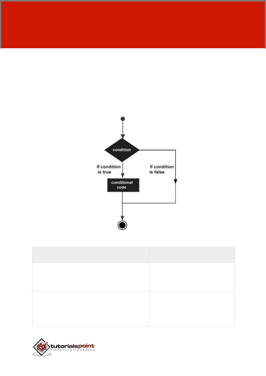
If the expression evaluates to true, then the block of code inside the if statement
will be executed. If the expression evaluates to false, then the first set of code
after the end statement will be executed.
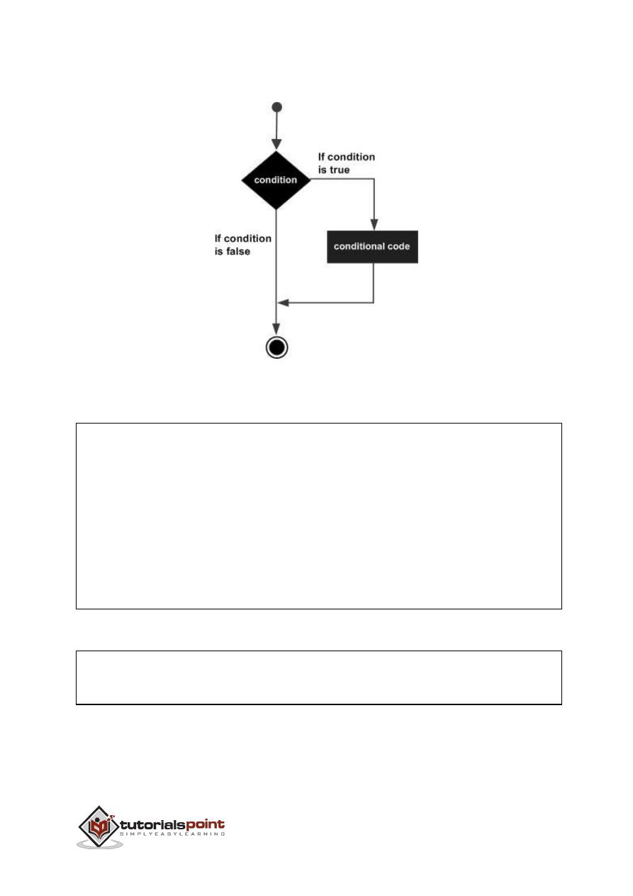
62
Flow Diagram
Example
Create a script file and type the following code:
a
=
10;
%
check the condition
using
if
statement
if
a
<
20
%
if
condition
is
true
then
the following
fprintf
('a is less than 20\n'
);
end
fprintf
('value of a is : %d\n',
a
);
When you run the file, it displays the following result:
a
is
less than
20
value of a
is
:
10
63
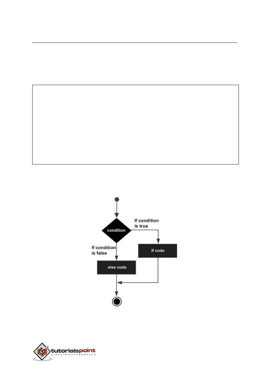
if...else...end Statement
An if statement can be followed by an optional else statement, which executes
when the expression is false.
Syntax
The syntax of an if...else statement in MATLAB is:
if
<expression>
%
statement
(
s
)
will execute
if
the
boolean
expression
is
true
<
statement
(
s
)>
else
<
statement
(
s
)>
%
statement
(
s
)
will execute
if
the
boolean
expression
is
false
end
If the boolean expression evaluates to true, then the if block of code will be
executed, otherwise else block of code will be executed.
Flow Diagram
Example
Create a script file and type the following code:

64
a
=
100;
%
check the
boolean
condition
if
a
<
20
%
if
condition
is
true
then
the following
fprintf
('a is less than 20\n'
);
else
%
if
condition
is
false
then
the following
fprintf
('a is not less than 20\n'
);
end
fprintf
('value of a is : %d\n',
a
);
When the above code is compiled and executed, it produces the following result:
a
is
not
less than
20
value of a
is
:
100
if...elseif...elseif...else...end Statements
An
if
statement can be followed by one (or more) optional
elseif...
and
an
else
statement, which is very useful to test various conditions.
When using if... elseif...else statements, there are few points to keep in mind:
An if can have zero or one else's and it must come after any elseif's.
An if can have zero to many elseif's and they must come before the else.
Once an else if succeeds, none of the remaining elseif's or else's will be tested.
Syntax
if
<
expression
1>
%
Executes
when
the expression
1
is
true
<
statement
(
s
)>
elseif
<
expression
2>
%
Executes
when
the
boolean
expression
2
is
true

65
<
statement
(
s
)>
Elseif
<
expression
3>
%
Executes
when
the
boolean
expression
3
is
true
<
statement
(
s
)>
else
%
executes
when
the none of the above condition
is
true
<
statement
(
s
)>
end
Example
Create a script file and type the following code in it:
a
=
100;
%
check the
boolean
condition
if
a
==
10
%
if
condition
is
true
then
the following
fprintf
('Value of a is 10\n'
);
elseif
(
a
==
20
)
%
if
else
if
condition
is
true
fprintf
('Value of a is 20\n'
);
elseif a
==
30
%
if
else
if
condition
is
true
fprintf
('Value of a is 30\n'
);
else
%
if
none of the conditions
is
true
'
fprintf('None
of the values are matching\n
');
fprintf('Exact
value of a
is:
%
d\n
', a );

66
end
When the above code is compiled and executed, it produces the following result:
None
of the values are matching
Exact
value of a
is:
100
The Nested if Statements
It is always legal in MATLAB to nest if-else statements which means you can use
one if or elseif statement inside another if or elseif statement(s).
Syntax
The syntax for a nested if statement is as follows:
if
<
expression
1>
%
Executes
when
the
boolean
expression
1
is
true
if
<
expression
2>
%
Executes
when
the
boolean
expression
2
is
true
end
end
You can nest elseif...else in the similar way as you have nested if statement.
Example
Create a script file and type the following code in it:
a
=
100;
b
=
200;
%
check the
boolean
condition
if(
a
==
100
)
%
if
condition
is
true
then
check the following
if(
b
==
200
)

67
%
if
condition
is
true
then
the following
fprintf
('Value of a is 100 and b is 200\n'
);
end
end
fprintf
('Exact value of a is : %d\n',
a
);
fprintf
('Exact value of b is : %d\n',
b
);
When you run the file, it displays:
Value
of a
is
100
and
b
is
200
Exact
value of a
is
:
100
Exact
value of b
is
:
200
The switch Statement
A switch block conditionally executes one set of statements from several choices.
Each choice is covered by a case statement.
An evaluated switch_expression is a scalar or string.
An evaluated case_expression is a scalar, a string or a cell array of scalars or
strings.
The switch block tests each case until one of the cases is true. A case is true when:
For numbers,
eq(case_expression,switch_expression).
For strings,
strcmp(case_expression,switch_expression).
For objects that support the eq function,eq(case_expression,switch_expression).
For a cell array case_expression, at least one of the elements of the cell array
matches switch_expression, as defined above for numbers, strings and objects.
When a case is true, MATLAB executes the corresponding statements and then
exits the switch block.
The
otherwise
block is optional and executes only when no case is true.
Syntax

68
The syntax of switch statement in MATLAB is:
switch
<switch_expression>
case
<case_expression>
<statements>
case
<case_expression>
<statements>
...
...
otherwise
<statements>
end
Example
Create a script file and type the following code in it:
grade
=
'B';
switch(
grade
)
case
'A'
fprintf
('Excellent!\n'
);
case
'B'
fprintf
('Well done\n'
);
case
'C'
fprintf
('Well done\n'
);
case
'D'
fprintf
('You passed\n'
);
case
'F'
fprintf
('Better try again\n'
);

69
otherwise
fprintf
('Invalid grade\n'
);
end
When you run the file, it displays:
Well
done
Your
grade
is
B
The Nested Switch Statements
It is possible to have a switch as part of the statement sequence of an outer
switch. Even if the case constants of the inner and outer switch contain common
values, no conflicts will arise.
Syntax
The syntax for a nested switch statement is as follows:
switch(
ch1
)
case
'A'
fprintf
('This A is part of outer switch');
switch(
ch2
)
case
'A'
fprintf
('This A is part of inner switch'
);
case
'B'
fprintf
('This B is part of inner switch'
);
end
case
'B'
fprintf
('This B is part of outer switch'
);
end

70
Example
Create a script file and type the following code in it:
a
=
100;
b
=
200;
switch(
a
)
case
100
fprintf
('This is part of outer switch %d\n',
a
);
switch(
b
)
case
200
fprintf
('This is part of inner switch %d\n',
a
);
end
end
fprintf
('Exact value of a is : %d\n',
a
);
fprintf
('Exact value of b is : %d\n',
b
);
When you run the file, it displays:
This
is
part of outer
switch
100
This
is
part of inner
switch
100
Exact
value of a
is
:
100
Exact
value of b
is
:
200
71
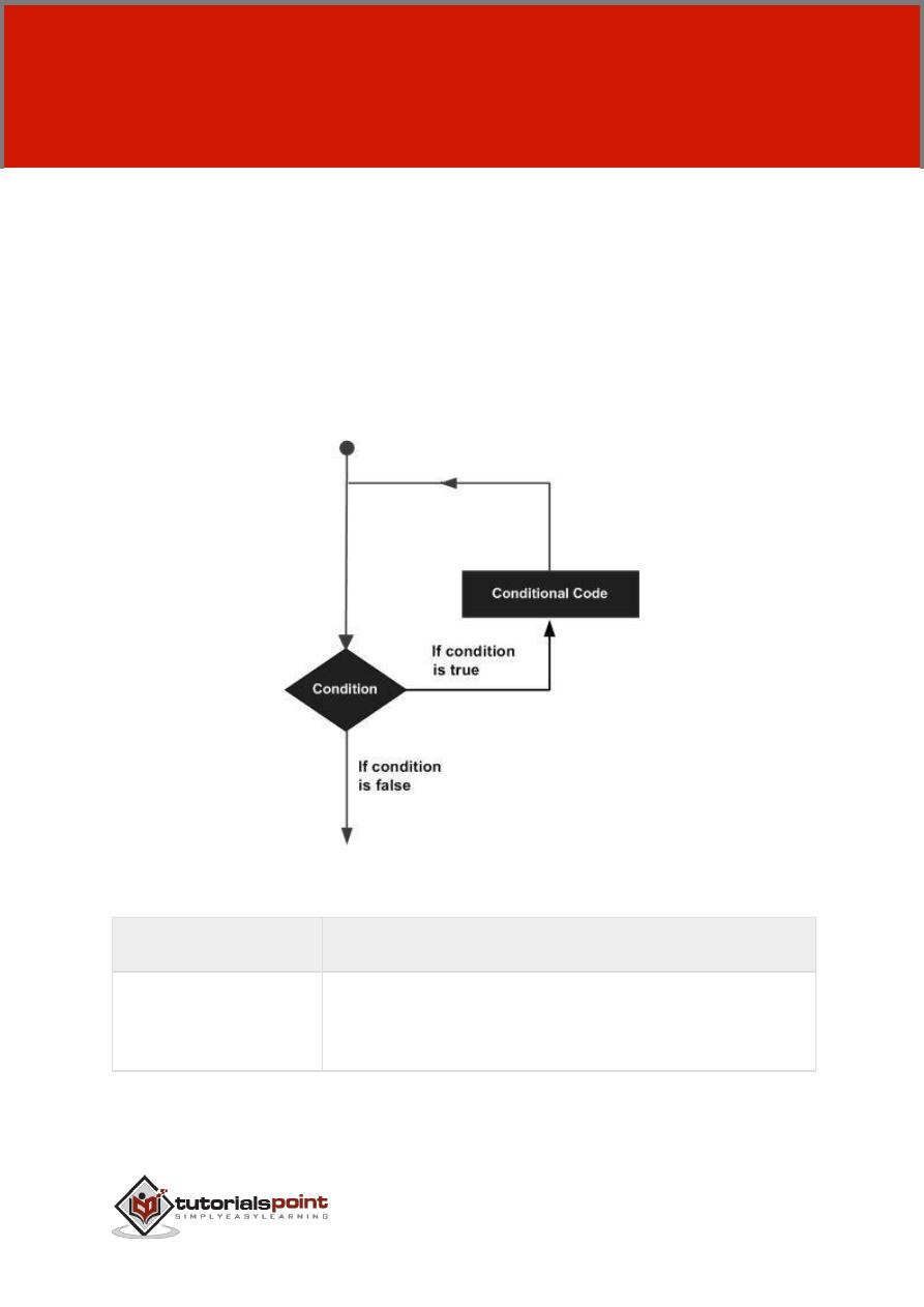
There may be a situation when you need to execute a block of code several
number of times. In general, statements are executed sequentially. The first
statement in a function is executed first, followed by the second, and so on.
Programming languages provide various control structures that allow for more
complicated execution paths.
A loop statement allows us to execute a statement or group of statements multiple
times and following is the general form of a loop statement in most of the
programming languages:
MATLAB provides following types of loops to handle looping requirements. Click
the following links to check their detail:
Loop Type
Description
while loop
Repeats a statement or group of statements while a
given condition is true. It tests the condition before
executing the loop body.
10.
LOOP TYPES

72
for loop
Executes a sequence of statements multiple times and
abbreviates the code that manages the loop variable.
nested loops
You can use one or more loops inside any another loop.
The while Loop
The while loop repeatedly executes statements while condition is true.
Syntax
The syntax of a while loop in MATLAB is:
while
<expression>
<statements>
end
The while loop repeatedly executes program statement(s) as long as the
expression remains true.
An expression is true when the result is nonempty and contains all nonzero
elements (logical or real numeric). Otherwise, the expression is false.
Example
Create a script file and type the following code:
a
=
10;
%
while
loop execution
while(
a
<
20
)
fprintf
('value of a: %d\n',
a
);
a
=
a
+
1;
end
When you run the file, it displays the following result:
value of a
:
10
value of a
:
11

73
value of a
:
12
value of a
:
13
value of a
:
14
value of a
:
15
value of a
:
16
value of a
:
17
value of a
:
18
value of a
:
19
The for Loop
A
for loop
is a repetition control structure that allows you to efficiently write a
loop that needs to execute a specific number of times.
Syntax
The syntax of a
for loop
in MATLAB is:
for
index
=
values
<
program statements
>
...
end
values
has one of the following forms:
Format
Description
initval:endval
increments the index variable from
initval
to
endval
by 1,
and
repeats
execution
of
program
statements
until
index
is greater than
endval.
initval:step:endval increments
index
by the value step on each iteration, or
decrements when step is negative.

74
valArray
creates a column vector
index
from subsequent columns
of arrayvalArray
on each iteration. For example, on the
first iteration, index = valArray(:,1). The loop executes
for a maximum of n times, where n is the number of
columns of
valArray, given by numel(valArray, 1, :). The
input
valArray
can be of any MATLAB data type, including
a string, cell array, or struct.
Example 1
Create a script file and type the following code:
for
a
=
10:20
fprintf
('value of a: %d\n',
a
);
end
When you run the file, it displays the following result:
value of a
:
10
value of a
:
11
value of a
:
12
value of a
:
13
value of a
:
14
value of a
:
15
value of a
:
16
value of a
:
17
value of a
:
18
value of a
:
19
value of a
:
20

75
Example 2
Create a script file and type the following code:
for
a
=
1.0:
-0.1:
0.0
disp
(
a
)
end
When you run the file, it displays the following result:
1
0.9000
0.8000
0.7000
0.6000
0.5000
0.4000
0.3000
0.2000
0.1000

76
0
Example 3
Create a script file and type the following code:
for
a
=
[24,18,17,23,28]
disp
(
a
)
end
When you run the file, it displays the following result:
24
18
17
23
28
The Nested Loops
MATLAB allows to use one loop inside another loop. Following section shows few
examples to illustrate the concept.
Syntax
The syntax for a nested for loop statement in MATLAB is as follows:
for
m
=
1:
j
for
n
=
1:
k
<statements>;
end

77
end
The syntax for a nested while loop statement in MATLAB is as follows:
while
<expression1>
while
<expression2>
<statements>
end
end
Example
Let us use a nested for loop to display all the prime numbers from 1 to 100. Create
a script file and type the following code:
for
i
=2:100
for
j
=2:100
if(~
mod
(
i
,
j
))
break;
%
if
factor found
,
not
prime
end
end
if(
j
>
(
i
/
j
))
fprintf
('%d is prime\n',
i
);
end
end
When you run the file, it displays the following result:
2
is
prime
3
is
prime
5
is
prime
7
is
prime

78
11
is
prime
13
is
prime
17
is
prime
19
is
prime
23
is
prime
29
is
prime
31
is
prime
37
is
prime
41
is
prime
43
is
prime
47
is
prime
53
is
prime
59
is
prime
61
is
prime
67
is
prime
71
is
prime
73
is
prime
79
is
prime
83
is
prime
89
is
prime
97
is
prime
Loop Control Statements
Loop control statements change execution from its normal sequence. When
execution leaves a scope, all automatic objects that were created in that scope
are destroyed.
MATLAB supports the following control statements. Click the following links to
check their detail.
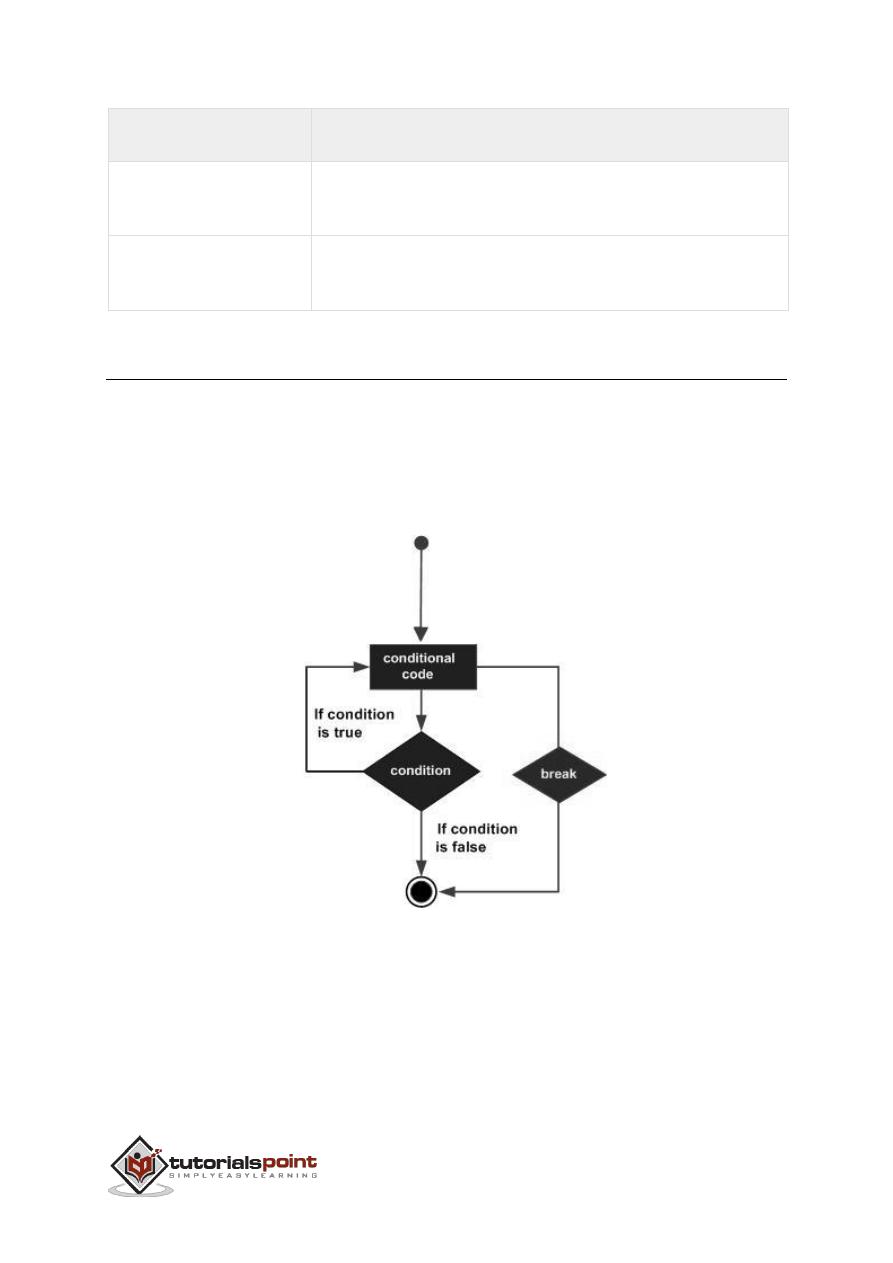
79
Control Statement
Description
break statement
Terminates the
loop
statement and transfers execution
to the statement immediately following the loop.
continue statement
Causes the loop to skip the remainder of its body and
immediately retest its condition prior to reiterating.
The break Statement
The break statement terminates execution of
for
or
while
loop. Statements in the
loop that appear after the break statement are not executed.
In nested loops, break exits only from the loop in which it occurs. Control passes
to the statement following the end of that loop.
Flow Diagram
Example
Create a script file and type the following code:

80
a
=
10;
%
while
loop execution
while
(
a
<
20
)
fprintf
('value of a: %d\n',
a
);
a
=
a
+1;
if(
a
>
15)
%
terminate the loop
using
break
statement
break;
end
end
When you run the file, it displays the following result:
value of a
:
10
value of a
:
11
value of a
:
12
value of a
:
13
value of a
:
14
value of a
:
15
The continue Statement
The continue statement is used for passing control to next iteration of for or while
loop.
The continue statement in MATLAB works somewhat like the break statement.
Instead of forcing termination, however, 'continue' forces the next iteration of the
loop to take place, skipping any code in between.
Flow Diagram
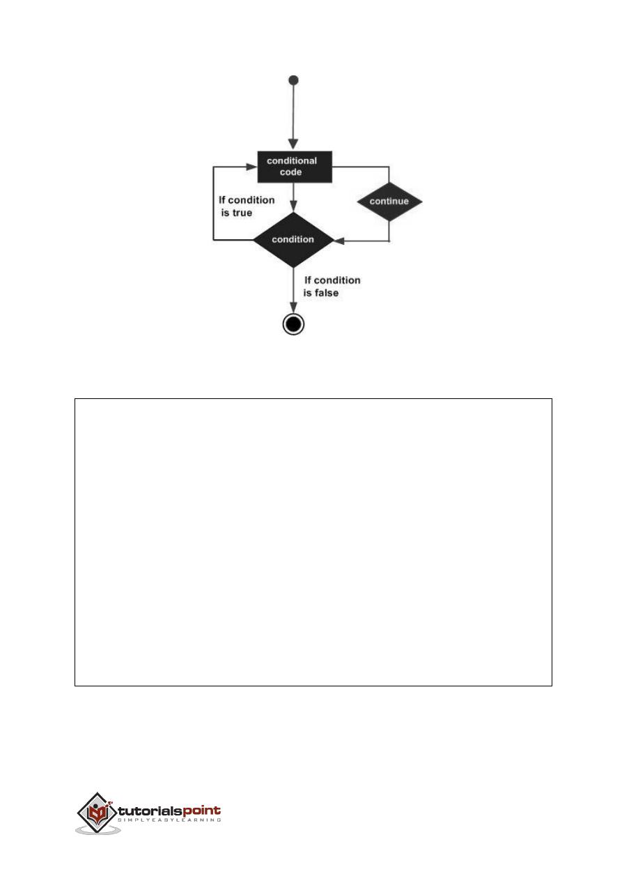
81
Example
Create a script file and type the following code:
a
=
10;
%while
loop execution
while
a
<
20
if
a
==
15
%
skip the iteration
a
=
a
+
1;
continue;
end
fprintf
('value of a: %d\n',
a
);
a
=
a
+
1;
end

82
When you run the file, it displays the following result:
value of a
:
10
value of a
:
11
value of a
:
12
value of a
:
13
value of a
:
14
value of a
:
16
value of a
:
17
value of a
:
18
value of a
:
19

83
A vector is a one-dimensional array of numbers. MATLAB allows creating two types
of vectors:
Row vectors
Column vectors
Row Vectors
Row vectors
are created by enclosing the set of elements in square brackets,
using space or comma to delimit the elements.
r
=
[7
8
9
10
11]
MATLAB will execute the above statement and return the following result:
r
=
Columns
1
through
4
7
8
9
10
Column
5
11
Column Vectors
Column vectors
are created by enclosing the set of elements in square brackets,
using semicolon to delimit the elements.
c
=
[7;
8;
9;
10;
11]
MATLAB will execute the above statement and return the following result:
c
=
7
8
11.
VECTORS

84
9
10
11
Referencing the Elements of a Vector
You can reference one or more of the elements of a vector in several ways. The
i
th
component of a vector v is referred as v(i). For example:
v
=
[
1;
2;
3;
4;
5;
6];
%
creating a column vector of
6
elements
v
(3)
MATLAB will execute the above statement and return the following result:
ans
=
3
When you reference a vector with a colon, such as v(:), all the components of the
vector are listed.
v
=
[
1;
2;
3;
4;
5;
6];
%
creating a column vector of
6
elements
v
(:)
MATLAB will execute the above statement and return the following result:
ans
=
1
2
3
4
5
6

85
MATLAB allows you to select a range of elements from a vector.
For example, let us create a row vector
rv
of 9 elements, then we will reference
the elements 3 to 7 by writing
rv(3:7)
and create a new vector named
sub_rv.
rv
=
[1
2
3
4
5
6
7
8
9];
sub_rv
=
rv
(3:7)
MATLAB will execute the above statement and return the following result:
sub_rv
=
3
4
5
6
7
Vector Operations
In this section, let us discuss the following vector operations:
Addition and Subtraction of Vectors
Scalar Multiplication of Vectors
Transpose of a Vector
Appending Vectors
Magnitude of a Vector
Vector Dot Product
Vectors with Uniformly Spaced Elements
Addition and Subtraction of Vectors
You can add or subtract two vectors. Both the operand vectors must be of same
type and have same number of elements.
Example
Create a script file with the following code:
A
=
[7,
11,
15,
23,
9];
B
=
[2,
5,
13,
16,
20];
C
=
A
+
B
;
D
=
A
-
B
;

86
disp
(
C
);
disp
(
D
);
When you run the file, it displays the following result:
9
16
28
39
29
5
6
2
7
-11
Scalar Multiplication of Vectors
When you multiply a vector by a number, this is called the
scalar multiplication.
Scalar multiplication produces a new vector of same type with each element of
the original vector multiplied by the number.
Example
Create a script file with the following code:
v
=
[
12
34
10
8];
m
=
5
*
v
When you run the file, it displays the following result:
m
=
60
170
50
40
Please note that you can perform all scalar operations on vectors. For example,
you can add, subtract and divide a vector with a scalar quantity.
Transpose of a Vector
The transpose operation changes a column vector into a row vector and vice versa.
The transpose operation is represented by a single quote (').
Example
Create a script file with the following code:
r
=
[
1
2
3
4
];
tr
=
r
';

87
v = [1;2;3;4];
tv = v';
disp
(
tr
);
disp
(
tv
);
When you run the file, it displays the following result:
1
2
3
4
1
2
3
4
Appending Vectors
MATLAB allows you to append vectors together to create new vectors.
If you have two row vectors r1 and r2 with n and m number of elements, to create
a row vector r of n plus m elements, by appending these vectors, you write:
r
=
[
r1
,
r2
]
You can also create a matrix r by appending these two vectors, the vector r2, will
be the second row of the matrix:
r
=
[
r1
;
r2
]
However, to do this, both the vectors should have same number of elements.
Similarly, you can append two column vectors c1 and c2 with n and m number of
elements. To create a column vector c of n plus m elements, by appending these
vectors, you write:
c
=
[
c1
;
c2
]
You can also create a matrix c by appending these two vectors; the vector c2 will
be the second column of the matrix:

88
c
=
[
c1
,
c2
]
However, to do this, both the vectors should have same number of elements.
Example
Create a script file with the following code:
r1
=
[
1
2
3
4
];
r2
=
[5
6
7
8
];
r
=
[
r1
,
r2
]
rMat
=
[
r1
;
r2
]
c1
=
[
1;
2;
3;
4
];
c2
=
[5;
6;
7;
8
];
c
=
[
c1
;
c2
]
cMat
=
[
c1
,
c2
]
When you run the file, it displays the following result:
r
=
1
2
3
4
5
6
7
8
rMat
=
1
2
3
4
5
6
7
8
c
=
1
2
3
4
5

89
6
7
8
cMat
=
1
5
2
6
3
7
4
8
Magnitude of a Vector
Magnitude of a vector v with elements v1, v2, v3, …, vn, is given by the equation:
|v| = √(v1
2
+ v2
2
+ v3
2
+ … + vn
2
)
You need to take the following steps to calculate the magnitude of a vector:
Take the product of the vector with itself, using
array multiplication
(.*). This
produces a vector sv, whose elements are squares of the elements of vector v.
sv = v.*v;
Use the sum function to get the
sum
of squares of elements of vector v. This is
also called the dot product of vector v.
dp= sum(sv);
Use the
sqrt
function to get the square root of the sum which is also the magnitude
of the vector v.
mag = sqrt(s);
Example
Create a script file with the following code:
v
=
[1:
2:
20];
sv
=
v
.*
v
;
%
the vector
with
elements
%
as
square of v
's elements
dp = sum(sv); % sum of squares -- the dot product
mag = sqrt(dp); % magnitude

90
disp('Magnitude:'); disp(mag);
When you run the file, it displays the following result:
Magnitude:
36.4692
Vector Dot Product
Dot product of two vectors a = (a1, a2, …, an) and b = (b1, b2, …, bn) is given
by:
a.b = ∑(ai.bi)
Dot product of two vectors a and b is calculated using the
dot
function.
dot
(
a
,
b
);
Example
Create a script file with the following code:
v1
=
[2
3
4];
v2
=
[1
2
3];
dp
=
dot
(
v1
,
v2
);
disp
('Dot Product:');
disp
(
dp
);
When you run the file, it displays the following result:
Dot
Product:
20
Vectors with Uniformly Spaced Elements
MATLAB allows you to create a vector with uniformly spaced elements.
To create a vector v with the first element f, last element l, and the difference
between elements is any real number n, we write:

91
v
=
[
f
:
n
:
l
]
Example
Create a script file with the following code:
v
=
[1:
2:
20];
sqv
=
v
.^2;
disp
(
v
);
disp
(
sqv
);
When you run the file, it displays the following result:
1
3
5
7
9
11
13
15
17
19
1
9
25
49
81
121
169
225
289
361

92
A matrix is a two-dimensional array of numbers.
In MATLAB, you create a matrix by entering elements in each row as comma or
space delimited numbers and using semicolons to mark the end of each row.
For example, let us create a 4-by-5 matrix
a:
a
=
[
1
2
3
4
5;
2
3
4
5
6;
3
4
5
6
7;
4
5
6
7
8]
MATLAB will execute the above statement and return the following result:
a
=
1
2
3
4
5
2
3
4
5
6
3
4
5
6
7
4
5
6
7
8
Referencing the Elements of a Matrix
To reference an element in the m
th
row and n
th
column, of a matrix
mx, we write:
mx
(
m
,
n
);
For example, to refer to the element in the 2
nd
row and 5
th
column, of the matrix
a,
as created in the last section, we type:
a
=
[
1
2
3
4
5;
2
3
4
5
6;
3
4
5
6
7;
4
5
6
7
8];
a
(2,5)
MATLAB will execute the above statement and return the following result:
ans
=
6
12.
MATRIX

93
To reference all the elements in the m
th
column we type A(:,m).
Let us create a column vector v, from the elements of the 4
th
row of the matrix a:
a
=
[
1
2
3
4
5;
2
3
4
5
6;
3
4
5
6
7;
4
5
6
7
8];
v
=
a
(:,4)
MATLAB will execute the above statement and return the following result:
v
=
4
5
6
7
You can also select the elements in the m
th
through n
th
columns, for this we write:
a
(:,
m
:
n
)
Let us create a smaller matrix taking the elements from the second and third
columns:
a
=
[
1
2
3
4
5;
2
3
4
5
6;
3
4
5
6
7;
4
5
6
7
8];
a
(:,
2:3)
MATLAB will execute the above statement and return the following result:
ans
=
2
3
3
4
4
5
5
6
In the same way, you can create a sub-matrix taking a sub-part of a matrix.
a
=
[
1
2
3
4
5;
2
3
4
5
6;
3
4
5
6
7;
4
5
6
7
8];

94
a
(:,
2:3)
MATLAB will execute the above statement and return the following result:
ans
=
2
3
3
4
4
5
5
6
In the same way, you can create a sub-matrix taking a sub-part of a matrix.
For example, let us create a sub-matrix
sa
taking the inner subpart of a:
3
4
5
4
5
6
To do this, write:
a
=
[
1
2
3
4
5;
2
3
4
5
6;
3
4
5
6
7;
4
5
6
7
8];
sa
=
a
(2:3,2:4)
MATLAB will execute the above statement and return the following result:
sa
=
3
4
5
4
5
6
Deleting a Row or a Column in a Matrix
You can delete an entire row or column of a matrix by assigning an empty set of
square braces [] to that row or column. Basically, [] denotes an empty array.
For example, let us delete the fourth row of a:
a
=
[
1
2
3
4
5;
2
3
4
5
6;
3
4
5
6
7;
4
5
6
7
8];

95
a
(
4
,
:
)
=
[]
MATLAB will execute the above statement and return the following result:
a
=
1
2
3
4
5
2
3
4
5
6
3
4
5
6
7
Next, let us delete the fifth column of a:
a
=
[
1
2
3
4
5;
2
3
4
5
6;
3
4
5
6
7;
4
5
6
7
8];
a
(:
,
5)=[]
MATLAB will execute the above statement and return the following result:
a
=
1
2
3
4
2
3
4
5
3
4
5
6
4
5
6
7
Example
In this example, let us create a 3-by-3 matrix m, then we will copy the second
and third rows of this matrix twice to create a 4-by-3 matrix.
Create a script file with the following code:
a
=
[
1
2
3
;
4
5
6;
7
8
9];
new_mat
=
a
([2,3,2,3],:)
When you run the file, it displays the following result:
new_mat
=
4
5
6

96
7
8
9
4
5
6
7
8
9
Matrix Operations
In this section, let us discuss the following basic and commonly used matrix
operations:
Addition and Subtraction of Matrices
Division of Matrices
Scalar Operations of Matrices
Transpose of a Matrix
Concatenating Matrices
Matrix Multiplication
Determinant of a Matrix
Inverse of a Matrix
Addition and Subtraction of Matrices
You can add or subtract matrices. Both the operand matrices must have the same
number of rows and columns.
Example
Create a script file with the following code:
a
=
[
1
2
3
;
4
5
6;
7
8
9];
b
=
[
7
5
6
;
2
0
8;
5
7
1];
c
=
a
+
b
d
=
a
-
b
When you run the file, it displays the following result:
c
=
8
7
9
6
5
14

97
12
15
10
d
=
-6
-3
-3
2
5
-2
2
1
8
Division (Left, Right) of Matrix
You can divide two matrices using left (\) or right (/) division operators. Both the
operand matrices must have the same number of rows and columns.
Example
Create a script file with the following code:
a
=
[
1
2
3
;
4
5
6;
7
8
9];
b
=
[
7
5
6
;
2
0
8;
5
7
1];
c
=
a
/
b
d
=
a \ b
When you run the file, it displays the following result:
c
=
-0.52542
0.68644
0.66102
-0.42373
0.94068
1.01695
-0.32203
1.19492
1.37288
d
=
-3.27778
-1.05556
-4.86111
-0.11111
0.11111
-0.27778

98
3.05556
1.27778
4.30556
Scalar Operations of Matrices
When you add, subtract, multiply or divide a matrix by a number, this is called
the
scalar operation.
Scalar operations produce a new matrix with same number of rows and columns
with each element of the original matrix added to, subtracted from, multiplied by
or divided by the number.
Example
Create a script file with the following code:
a
=
[
10
12
23
;
14
8
6;
27
8
9];
b
=
2;
c
=
a
+
b
d
=
a
-
b
e
=
a
*
b
f
=
a
/
b
When you run the file, it displays the following result:
c
=
12
14
25
16
10
8
29
10
11
d
=
8
10
21
12
6
4
25
6
7
e
=
20
24
46

99
28
16
12
54
16
18
f
=
5.0000
6.0000
11.5000
7.0000
4.0000
3.0000
13.5000
4.0000
4.5000
Transpose of a Matrix
The transpose operation switches the rows and columns in a matrix. It is
represented by a single quote(').
Example
Create a script file with the following code:
a
=
[
10
12
23
;
14
8
6;
27
8
9]
b
=
a
'
When you run the file, it displays the following result:
a
=
10
12
23
14
8
6
27
8
9
b
=
10
14
27
12
8
8
23
6
9
Concatenating Matrices
You can concatenate two matrices to create a larger matrix. The pair of square
brackets '[]' is the concatenation operator.

100
MATLAB allows two types of concatenations:
Horizontal concatenation
Vertical concatenation
When you concatenate two matrices by separating those using commas, they are
just appended horizontally. It is called horizontal concatenation.
Alternatively, if you concatenate two matrices by separating those using
semicolons, they are appended vertically. It is called vertical concatenation.
Example
Create a script file with the following code:
a
=
[
10
12
23
;
14
8
6;
27
8
9]
b
=
[
12
31
45
;
8
0
-9;
45
2
11]
c
=
[
a
,
b
]
d
=
[
a
;
b
]
When you run the file, it displays the following result:
a
=
10
12
23
14
8
6
27
8
9
b
=
12
31
45
8
0
-9
45
2
11
c
=
10
12
23
12
31
45
14
8
6
8
0
-9
27
8
9
45
2
11
d
=

101
10
12
23
14
8
6
27
8
9
12
31
45
8
0
-9
45
2
11
Matrix Multiplication
Consider two matrices A and B. If A is an m x n matrix and B is an n x p matrix,
they could be multiplied together to produce an m x n matrix C. Matrix
multiplication is possible only if the number of columns n in A is equal to the
number of rows n in B.
In matrix multiplication, the elements of the rows in the first matrix are multiplied
with corresponding columns in the second matrix.
Each element in the (i, j)
th
position, in the resulting matrix C, is the summation of
the products of elements in i
th
row of first matrix with the corresponding element
in the j
th
column of the second matrix.
Matrix multiplication in MATLAB is performed by using the * operator.
Example
Create a script file with the following code:
a
=
[
1
2
3;
2
3
4;
1
2
5]
b
=
[
2
1
3
;
5
0
-2;
2
3
-1]
prod
=
a
*
b
When you run the file, it displays the following result:
a
=
1
2
3
2
3
4
1
2
5

102
b
=
2
1
3
5
0
-2
2
3
-1
prod
=
18
10
-4
27
14
-4
22
16
-6
Determinant of a Matrix
Determinant of a matrix is calculated using the
det
function of MATLAB.
Determinant of a matrix A is given by det(A).
Example
Create a script file with the following code:
a
=
[
1
2
3;
2
3
4;
1
2
5]
det
(
a
)
When you run the file, it displays the following result:
a
=
1
2
3
2
3
4
1
2
5
ans
=
-2
Inverse of a Matrix
The inverse of a matrix A is denoted by A
−1
such that the following relationship
holds:

103
AA
−1
=
A
−1A
=
1
The inverse of a matrix does not always exist.
If the determinant of the matrix is
zero, then the inverse does not exist and the matrix is singular.
Inverse of a matrix in MATLAB is calculated using the
inv
function. Inverse of a
matrix A is given by inv(A).
Example
Create a script file and type the following code:
a
=
[
1
2
3;
2
3
4;
1
2
5]
inv
(
a
)
When you run the file, it displays the following result:
a
=
1
2
3
2
3
4
1
2
5
ans
=
-3.5000
2.0000
0.5000
3.0000
-1.0000
-1.0000
-0.5000
0
0.5000

104
All variables of all data types in MATLAB are multidimensional arrays. A vector is
a one-dimensional array and a matrix is a two-dimensional array.
We have already discussed vectors and matrices. In this chapter, we will discuss
multidimensional arrays. However, before that, let us discuss some special types
of arrays.
Special Arrays in MATLAB
In this section, we will discuss some functions that create some special arrays. For
all these functions, a single argument creates a square array, double arguments
create rectangular array.
The
zeros()
function creates an array of all zeros:
For example:
zeros
(5)
MATLAB will execute the above statement and return the following result:
ans
=
0
0
0
0
0
0
0
0
0
0
0
0
0
0
0
0
0
0
0
0
0
0
0
0
0
The
ones()
function creates an array of all ones:
For example:
ones
(4,3)
MATLAB will execute the above statement and return the following result:
13.
ARRAYS

105
ans
=
1
1
1
1
1
1
1
1
1
1
1
1
The
eye()
function creates an identity matrix.
For example:
eye
(4)
MATLAB will execute the above statement and return the following result:
ans
=
1
0
0
0
0
1
0
0
0
0
1
0
0
0
0
1
The
rand()
function creates an array of uniformly distributed random numbers on
(0,1):
For example:
rand
(3,
5)
MATLAB will execute the above statement and return the following result:
ans
=
0.8147
0.9134
0.2785
0.9649
0.9572
0.9058
0.6324
0.5469
0.1576
0.4854
0.1270
0.0975
0.9575
0.9706
0.8003

106
A Magic Square
A
magic square
is a square that produces the same sum, when its elements are
added row-wise, column-wise or diagonally.
The
magic()
function creates a magic square array. It takes a singular argument
that gives the size of the square. The argument must be a scalar greater than or
equal to 3.
magic
(4)
MATLAB will execute the above statement and return the following result:
ans
=
16
2
3
13
5
11
10
8
9
7
6
12
4
14
15
1
Multidimensional Arrays
An array having more than two dimensions is called a multidimensional array in
MATLAB. Multidimensional arrays in MATLAB are an extension of the normal two-
dimensional matrix.
Generally to generate a multidimensional array, we first create a two-dimensional
array and extend it.
For example, let's create a two-dimensional array a.
a
=
[7
9
5;
6
1
9;
4
3
2]
MATLAB will execute the above statement and return the following result:
a
=
7
9
5
6
1
9
4
3
2

107
The array
a
is a 3-by-3 array; we can add a third dimension to
a, by providing the
values like:
a
(:,
:,
2)=
[
1
2
3;
4
5
6;
7
8
9]
MATLAB will execute the above statement and return the following result:
a
(:,:,1)
=
7
9
5
6
1
9
4
3
2
a
(:,:,2)
=
1
2
3
4
5
6
7
8
9
We can also create multidimensional arrays using the ones(), zeros() or the rand()
functions.
For example,
b
=
rand
(4,3,2)
MATLAB will execute the above statement and return the following result:
b
(:,:,1)
=
0.0344
0.7952
0.6463
0.4387
0.1869
0.7094
0.3816
0.4898
0.7547
0.7655
0.4456
0.2760
b
(:,:,2)
=
0.6797
0.4984
0.2238

108
0.6551
0.9597
0.7513
0.1626
0.3404
0.2551
0.1190
0.5853
0.5060
We can also use the
cat()
function to build multidimensional arrays. It
concatenates a list of arrays along a specified dimension:
Syntax for the cat() function is:
B
=
cat
(
dim
,
A1
,
A2
...)
Where,
B
is the new array created
A1,
A2, ... are the arrays to be concatenated
dim
is the dimension along which to concatenate the arrays
Example
Create a script file and type the following code into it:
a
=
[9
8
7;
6
5
4;
3
2
1];
b
=
[1
2
3;
4
5
6;
7
8
9];
c
=
cat
(3,
a
,
b
,
[
2
3
1;
4
7
8;
3
9
0])
When you run the file, it displays:
c
(:,:,1)
=
9
8
7
6
5
4
3
2
1
c
(:,:,2)
=
1
2
3
4
5
6
7
8
9
c
(:,:,3)
=

109
2
3
1
4
7
8
3
9
0
Array Functions
MATLAB provides the following functions to sort, rotate, permute, reshape, or shift
array contents.
Function
Purpose
length
Length of vector or largest array dimension
ndims
Number of array dimensions
numel
Number of array elements
size
Array dimensions
iscolumn
Determines whether input is column vector
isempty
Determines whether array is empty
ismatrix
Determines whether input is matrix
isrow
Determines whether input is row vector
isscalar
Determines whether input is scalar
isvector
Determines whether input is vector
blkdiag
Constructs block diagonal matrix from input arguments
circshift
Shifts array circularly
ctranspose
Complex conjugate transpose

110
diag
Diagonal matrices and diagonals of matrix
flipdim
Flips array along specified dimension
fliplr
Flips matrix from left to right
flipud
Flips matrix up to down
ipermute
Inverses permute dimensions of N-D array
permute
Rearranges dimensions of N-D array
repmat
Replicates and tile array
reshape
Reshapes array
rot90
Rotates matrix 90 degrees
shiftdim
Shifts dimensions
issorted
Determines whether set elements are in sorted order
sort
Sorts array elements in ascending or descending order
sortrows
Sorts rows in ascending order
squeeze
Removes singleton dimensions
transpose
Transpose
vectorize
Vectorizes expression
Examples
The following examples illustrate some of the functions mentioned above.
Length, Dimension and Number of elements:
Create a script file and type the following code into it:

111
x
=
[7.1,
3.4,
7.2,
28/4,
3.6,
17,
9.4,
8.9];
length
(
x
)
%
length of x vector
y
=
rand
(3,
4,
5,
2);
ndims
(
y
)
%
no
of dimensions
in
array y
s
=
['Zara',
'Nuha',
'Shamim',
'Riz',
'Shadab'];
numel
(
s
)
%
no
of elements
in
s
When you run the file, it displays the following result:
ans
=
8
ans
=
4
ans
=
23
Circular Shifting of the Array Elements:
Create a script file and type the following code into it:
a
=
[1
2
3;
4
5
6;
7
8
9]
%
the original array a
b
=
circshift
(
a
,1)
%
circular shift first dimension values down
by
1.
c
=
circshift
(
a
,[1
-1])
%
circular shift first dimension values
%
down
by
1
%
and
second dimension values to the left
%
by
1.
When you run the file, it displays the following result:
a
=
1
2
3
4
5
6
7
8
9

112
b
=
7
8
9
1
2
3
4
5
6
c
=
8
9
7
2
3
1
5
6
4
Sorting Arrays
Create a script file and type the following code into it:
v
=
[
23
45
12
9
5
0
19
17]
%
horizonal vector
sort
(
v
)
%
sorting v
m
=
[2
6
4;
5
3
9;
2
0
1]
%
two dimensional array
sort
(
m
,
1)
%
sorting m along the row
sort
(
m
,
2)
%
sorting m along the column
When you run the file, it displays the following result:
v
=
23
45
12
9
5
0
19
17
ans
=
0
5
9
12
17
19
23
45
m
=
2
6
4
5
3
9
2
0
1

113
ans
=
2
0
1
2
3
4
5
6
9
ans
=
2
4
6
3
5
9
0
1
2
Cell Array
Cell arrays are arrays of indexed cells where each cell can store an array of a
different dimensions and data types.
The
cell
function is used for creating a cell array. Syntax for the cell function is:
C
=
cell
(
dim
)
C
=
cell
(
dim1
,...,
dimN
)
D
=
cell
(
obj
)
Where,
C
is the cell array;
dim
is a scalar integer or vector of integers that specifies the dimensions of cell
array C;
dim1, ... , dimN
are scalar integers that specify the dimensions of C;
obj
is One of the following:
Java array or object
.NET array of type System.String or System.Object
Example
Create a script file and type the following code into it:
c
=
cell
(2,
5);
c
=
{'Red',
'Blue',
'Green',
'Yellow',
'White';
1
2
3
4
5}

114
When you run the file, it displays the following result:
c
=
'Red'
'Blue'
'Green'
'Yellow'
'White'
[
1]
[
2]
[
3]
[
4]
[
5]
Accessing Data in Cell Arrays
There are two ways to refer to the elements of a cell array:
Enclosing the indices in first bracket (), to refer to sets of cells
Enclosing the indices in braces {}, to refer to the data within individual cells
When you enclose the indices in first bracket, it refers to the set of cells.
Cell array indices in smooth parentheses refer to sets of cells.
For example:
c
=
{'Red',
'Blue',
'Green',
'Yellow',
'White';
1
2
3
4
5};
c
(1:2,1:2)
MATLAB will execute the above statement and return the following result:
ans
=
'Red'
'Blue'
[
1]
[
2]
You can also access the contents of cells by indexing with curly braces.
For example:
c
=
{'Red',
'Blue',
'Green',
'Yellow',
'White';
1
2
3
4
5};
c
{1,
2:4}
MATLAB will execute the above statement and return the following result:
ans
=
Blue

115
ans
=
Green
ans
=
Yellow

116
The
colon(:)
is one of the most useful operator in MATLAB. It is used to create
vectors, subscript arrays, and specify for iterations.
If you want to create a row vector, containing integers from 1 to 10, you write:
1:10
MATLAB executes the statement and returns a row vector containing the integers
from 1 to 10:
ans
=
1
2
3
4
5
6
7
8
9
10
If you want to specify an increment value other than one, for example:
100:
-5:
50
MATLAB executes the statement and returns the following result:
ans
=
100
95
90
85
80
75
70
65
60
55
50
Let us take another example:
0:
pi
/8:
pi
MATLAB executes the statement and returns the following result:
ans
=
Columns
1
through
7
0
0.3927
0.7854
1.1781
1.5708
1.9635
2.3562
Columns
8
through
9
2.7489
3.1416
14.
COLON NOTATION
117
You can use the colon operator to create a vector of indices to select rows, columns
or elements of arrays.
The following table describes its use for this purpose (let us have a matrix A):
Format
Purpose
A(:,j)
is the jth column of A.
A(i,:)
is the ith row of A.
A(:,:)
is the equivalent two-dimensional array. For matrices this is the
same as A.
A(j:k)
is A(j), A(j+1),...,A(k).
A(:,j:k)
is A(:,j), A(:,j+1),...,A(:,k).
A(:,:,k)
is the k
th
page of three-dimensional array A.
A(i,j,k,:) is a vector in four-dimensional array A. The vector includes
A(i,j,k,1), A(i,j,k,2), A(i,j,k,3), and so on.
A(:)
is all the elements of A, regarded as a single column. On the left
side of an assignment statement, A(:) fills A, preserving its shape
from before. In this case, the right side must contain the same
number of elements as A.
Example
Create a script file and type the following code in it:
A
=
[1
2
3
4;
4
5
6
7;
7
8
9
10]
A
(:,2)
%
second column of A
A
(:,2:3)
%
second
and
third column of A
A
(2:3,2:3)
%
second
and
third rows
and
second
and
third columns

118
When you run the file, it displays the following result:
A
=
1
2
3
4
4
5
6
7
7
8
9
10
ans
=
2
5
8
ans
=
2
3
5
6
8
9
ans
=
5
6
8
9

119
MATLAB supports various numeric classes that include signed and unsigned
integers and single-precision and double-precision floating-point numbers. By
default, MATLAB stores all numeric values as double-precision floating point
numbers.
You can choose to store any number or array of numbers as integers or as single-
precision numbers.
All numeric types support basic array operations and mathematical operations.
Conversion to Various Numeric Data Types
MATLAB provides the following functions to convert to various numeric data types:
Function
Purpose
Double
Converts to double precision number
Single
Converts to single precision number
int8
Converts to 8-bit signed integer
int16
Converts to 16-bit signed integer
int32
Converts to 32-bit signed integer
int64
Converts to 64-bit signed integer
uint8
Converts to 8-bit unsigned integer
uint16
Converts to 16-bit unsigned integer
uint32
Converts to 32-bit unsigned integer
uint64
Converts to 64-bit unsigned integer
15.
NUMBERS

120
Example
Create a script file and type the following code:
x
=
single
([5.32
3.47
6.28])
.*
7.5
x
=
double([5.32
3.47
6.28])
.*
7.5
x
=
int8
([5.32
3.47
6.28])
.*
7.5
x
=
int16
([5.32
3.47
6.28])
.*
7.5
x
=
int32
([5.32
3.47
6.28])
.*
7.5
x
=
int64
([5.32
3.47
6.28])
.*
7.5
When you run the file, it shows the following result:
x
=
39.9000
26.0250
47.1000
x
=
39.9000
26.0250
47.1000
x
=
38
23
45
x
=
38
23
45
x
=
38
23
45
x
=
38
23
45
Example
Let us extend the previous example a little more. Create a script file and type the
following code:
x
=
int32
([5.32
3.47
6.28])
.*
7.5

121
x
=
int64
([5.32
3.47
6.28])
.*
7.5
x
=
num2cell
(
x
)
When you run the file, it shows the following result:
x
=
38
23
45
x
=
38
23
45
x
=
[38]
[23]
[45]
Smallest and Largest Integers
The functions
intmax()
and
intmin()
return the maximum and minimum values
that can be represented with all types of integer numbers.
Both the functions take the integer data type as the argument, for example,
intmax(int8) or intmin(int64) and return the maximum and minimum values that
you can represent with the integer data type.
Example
The following example illustrates how to obtain the smallest and largest values of
integers. Create a script file and write the following code in it:
%
displaying the smallest
and
largest
signed
integer data
str
=
'The range for int8 is:\n\t%d to %d ';
sprintf
(
str
,
intmin
('int8'),
intmax
('int8'))
str
=
'The range for int16 is:\n\t%d to %d ';
sprintf
(
str
,
intmin
('int16'),
intmax
('int16'))
str
=
'The range for int32 is:\n\t%d to %d ';
sprintf
(
str
,
intmin
('int32'),
intmax
('int32'))
str
=
'The range for int64 is:\n\t%d to %d ';

122
sprintf
(
str
,
intmin
('int64'),
intmax
('int64'))
%
displaying the smallest
and
largest
unsigned
integer data
str
=
'The range for uint8 is:\n\t%d to %d ';
sprintf
(
str
,
intmin
('uint8'),
intmax
('uint8'))
str
=
'The range for uint16 is:\n\t%d to %d ';
sprintf
(
str
,
intmin
('uint16'),
intmax
('uint16'))
str
=
'The range for uint32 is:\n\t%d to %d ';
sprintf
(
str
,
intmin
('uint32'),
intmax
('uint32'))
str
=
'The range for uint64 is:\n\t%d to %d ';
sprintf
(
str
,
intmin
('uint64'),
intmax
('uint64'))
When you run the file, it shows the following result:
ans
=
The
range
for
int8
is:
-128
to
127
ans
=
The
range
for
int16
is:
-32768
to
32767
ans
=
The
range
for
int32
is:
-2147483648
to
2147483647
ans
=
The
range
for
int64
is:
-9223372036854775808
to
9223372036854775807
ans
=
The
range
for
uint8
is:

123
0
to
255
ans
=
The
range
for
uint16
is:
0
to
65535
ans
=
The
range
for
uint32
is:
0
to
4294967295
ans
=
The
range
for
uint64
is:
0
to
1.844674e+19
Smallest and Largest Floating Point Numbers
The functions
realmax()
and
realmin()
return the maximum and minimum
values that can be represented with floating point numbers.
Both the functions when called with the argument 'single', return the maximum
and minimum values that you can represent with the single-precision data type
and when called with the argument 'double', return the maximum and minimum
values that you can represent with the double-precision data type.
Example
The following example illustrates how to obtain the smallest and largest floating
point numbers. Create a script file and write the following code in it:
%
displaying the smallest
and
largest single
-
precision
%
floating point number
str
=
'The range for single is:\n\t%g to %g and\n\t %g to %g';
sprintf
(
str
,
-
realmax
('single'),
-
realmin
('single'),
...
realmin
('single'),
realmax
('single'))
%
displaying the smallest
and
largest
double-
precision
%
floating point number

124
str
=
'The range for double is:\n\t%g to %g and\n\t %g to %g';
sprintf
(
str
,
-
realmax
('double'),
-
realmin
('double'),
...
realmin
('double'),
realmax
('double'))
When you run the file, it displays the following result:
ans
=
The
range
for
single
is:
-3.40282e+38
to
-1.17549e-38
and
1.17549e-38
to
3.40282e+38
ans
=
The
range
for
double
is:
-1.79769e+308
to
-2.22507e-308
and
2.22507e-308
to
1.79769e+308

125
Creating a character string is quite simple in MATLAB. In fact, we have used it
many times. For example, you type the following in the command prompt:
my_string
=
'Tutorial''s Point'
MATLAB will execute the above statement and return the following result:
my_string
=
Tutorial's Point
MATLAB considers all variables as arrays, and strings are considered as character
arrays. Let us use the whos command to check the variable created above:
whos
MATLAB will execute the above statement and return the following result:
Name
Size
Bytes
Class
Attributes
my_string
1x16
32
char
Interestingly, you can use numeric conversion functions like
uint8
or
uint16
to
convert the characters in the string to their numeric codes. The
char
function
converts the integer vector back to characters:
Example
Create a script file and type the following code into it:
my_string
=
'Tutorial''s Point'
;
str_ascii
=
uint8
(
my_string
)
%
8
-
bit ascii values
str_back_to_char
=
char
(
str_ascii
)
str_16bit
=
uint16
(
my_string
)
%
16
-
bit ascii values
str_back_to_char
=
char
(
str_16bit
)
16.
STRINGS

126
When you run the file, it displays the following result:
str_ascii
=
Columns
1
through
14
84
117
116
111
114
105
97
108
39
115
32
80
111
105
Columns
15
through
16
110
116
str_back_to_char
=
Tutorial's Point
str_16bit =
Columns 1 through 10
84 117 116 111 114 105 97 108 39 115
Columns 11 through 16
32 80 111 105 110 116
str_back_to_char =
Tutorial'
s
Point
Rectangular Character Array
The strings we have discussed so far are one-dimensional character arrays;
however, we need to store more than that. We need to store more dimensional
textual data in our program. This is achieved by creating rectangular character
arrays.
Simplest way of creating a rectangular character array is by concatenating two or
more one-dimensional character arrays, either vertically or horizontally as
required.
You can combine strings vertically in either of the following ways:
Using the MATLAB concatenation operator
[]
and separating each row with a
semicolon (;).Please note that in this method each row must contain the same
number of characters. For strings with different lengths, you should pad with space
characters as needed.

127
Using the
char
function. If the strings are of different lengths, char pads the
shorter strings with trailing blanks so that each row has the same number of
characters.
Example
Create a script file and type the following code into it:
doc_profile
=
['Zara Ali ';
...
'Sr. Surgeon ';
...
'R N Tagore Cardiology Research Center']
doc_profile
=
char('Zara Ali',
'Sr. Surgeon',
...
'RN Tagore Cardiology Research Center')
When you run the file, it displays the following result:
doc_profile
=
Zara
Ali
Sr.
Surgeon
R N
Tagore
Cardiology
Research
Center
doc_profile
=
Zara
Ali
Sr.
Surgeon
RN
Tagore
Cardiology
Research
Center
You can combine strings horizontally in either of the following ways:
Using the MATLAB concatenation operator,
[]
and separating the input strings with
a comma or a space. This method preserves any trailing spaces in the input arrays.
Using the string concatenation function,
strcat. This method removes trailing
spaces in the inputs
Example
Create a script file and type the following code into it:
name
=
'Zara Ali ';
position
=
'Sr. Surgeon ';

128
worksAt
=
'R N Tagore Cardiology Research Center';
profile
=
[
name
', '
position
', '
worksAt
]
profile
=
strcat
(
name
,
', ',
position
,
', ',
worksAt
)
When you run the file, it displays the following result:
profile
=
Zara
Ali
,
Sr.
Surgeon
,
R N
Tagore
Cardiology
Research
Center
profile
=
Zara
Ali,Sr.
Surgeon,
R N
Tagore
Cardiology
Research
Center
Combining Strings into a Cell Array
From our previous discussion, it is clear that combining strings with different
lengths could be a pain as all strings in the array has to be of the same length.
We have used blank spaces at the end of strings to equalize their length.
However, a more efficient way to combine the strings is to convert the resulting
array into a cell array.
MATLAB cell array can hold different sizes and types of data in an array. Cell arrays
provide a more flexible way to store strings of varying length.
The
cellstr
function converts a character array into a cell array of strings.
Example
Create a script file and type the following code into it:
name
=
'Zara Ali ';
position
=
'Sr. Surgeon ';
worksAt
=
'R N Tagore Cardiology Research Center';
profile
=
char(
name
,
position
,
worksAt
);
profile
=
cellstr
(
profile
);
disp
(
profile
)
When you run the file, it displays the following result:

129
'Zara Ali'
'Sr. Surgeon'
'R N Tagore Cardiology Research Center'
String Functions in MATLAB
MATLAB provides numerous string functions creating, combining, parsing,
comparing and manipulating strings.
Following table provides brief description of the string functions in MATLAB:
Function
Purpose
Functions for storing text in character arrays, combine character arrays, etc.
blanks
Create string of blank characters
cellstr
Create cell array of strings from character array
char
Convert to character array (string)
iscellstr
Determine whether input is cell array of strings
ischar
Determine whether item is character array
sprintf
Format data into string
strcat
Concatenate strings horizontally
strjoin
Join strings in cell array into single string
Functions for identifying parts of strings, find and replace substrings
ischar
Determine whether item is character array
isletter
Array elements that are alphabetic letters

130
isspace
Array elements that are space characters
isstrprop
Determine whether string is of specified category
sscanf
Read formatted data from string
strfind
Find one string within another
strrep
Find and replace substring
strsplit
Split string at specified delimiter
strtok
Selected parts of string
validatestring
Check validity of text string
symvar
Determine symbolic variables in expression
regexp
Match regular expression (case sensitive)
regexpi
Match regular expression (case insensitive)
regexprep
Replace string using regular expression
regexptranslate
Translate string into regular expression
Functions for string comparison
strcmp
Compare strings (case sensitive)
strcmpi
Compare strings (case insensitive)
strncmp
Compare first n characters of strings (case sensitive)
strncmpi
Compare first n characters of strings (case
insensitive)

131
Functions for changing string to upper- or lowercase, creating or
removing white space
deblank
Strip trailing blanks from end of string
strtrim
Remove leading and trailing white space from string
lower
Convert string to lowercase
upper
Convert string to uppercase
strjust
Justify character array
Examples
The following examples illustrate some of the above-mentioned string functions:
Formatting Strings
Create a script file and type the following code into it:
A
=
pi
*1000*
ones
(1,5);
sprintf
(' %f \n %.2f \n %+.2f \n %12.2f \n %012.2f \n',
A
)
When you run the file, it displays the following result:
ans
=
3141.592654
3141.59
+3141.59
3141.59
000003141.59
Joining Strings
Create a script file and type the following code into it:
%
cell array of strings

132
str_array
=
{
'red'
,
'blue'
,
'green'
,
'yellow'
,
'orange'
};
%
Join
strings
in
cell array
into
single
string
str1
=
strjoin
(
"-"
,
str_array
)
str2
=
strjoin
(
","
,
str_array
)
When you run the file, it displays the following result:
str1
=
red blue green yellow orange
str2
=
red
,
blue
,
green
,
yellow
,
orange
Finding and Replacing Strings
Create a script file and type the following code into it:
students
=
{'Zara Ali',
'Neha Bhatnagar',
...
'Monica Malik',
'Madhu Gautam',
...
'Madhu Sharma',
'Bhawna Sharma',...
'Nuha Ali',
'Reva Dutta',
...
'Sunaina Ali',
'Sofia Kabir'};
%
The
strrep
function
searches
and
replaces
sub-string.
new_student
=
strrep
(
students
(8),
'Reva',
'Poulomi')
%
Display
first names
first_names
=
strtok
(
students
)
When you run the file, it displays the following result:
new_student
=

133
'Poulomi Dutta'
first_names
=
Columns
1
through
6
'Zara'
'Neha'
'Monica'
'Madhu'
'Madhu'
'Bhawna'
Columns
7
through
10
'Nuha'
'Reva'
'Sunaina'
'Sofia'
Comparing Strings
Create a script file and type the following code into it:
str1
=
'This is test'
str2
=
'This is text'
if
(
strcmp
(
str1
,
str2
))
sprintf
('%s and %s are equal',
str1
,
str2
)
else
sprintf
('%s and %s are not equal',
str1
,
str2
)
end
When you run the file, it displays the following result:
str1
=
This
is
test
str2
=
This
is
text
ans
=
This
is
test
and
This
is
text are
not
equal

134
A function is a group of statements that together perform a task. In MATLAB,
functions are defined in separate files. The name of the file and of the function
should be the same.
Functions operate on variables within their own workspace, which is also called
the
local workspace, separate from the workspace you access at the MATLAB
command prompt which is called the
base workspace.
Functions can accept more than one input arguments and may return more than
one output arguments
Syntax of a function statement is:
function
[
out1
,
out2
,
...,
outN
]
=
myfun
(
in1
,
in2
,
in3
,
...,
inN
)
Example
The following function named
mymax
should be written in a file named
mymax.m.
It takes five numbers as argument and returns the maximum of the numbers.
Create a function file, named mymax.m and type the following code in it:
function
max
=
mymax
(
n1
,
n2
,
n3
,
n4
,
n5
)
%This
function
calculates the maximum of the
%
five numbers given
as
input
max
=
n1
;
if(
n2
>
max
)
max
=
n2
;
end
if(
n3
>
max
)
max
=
n3
;
end
if(
n4
>
max
)
max
=
n4
;
17.
FUNCTIONS

135
end
if(
n5
>
max
)
max
=
n5
;
end
The first line of a function starts with the keyword
function. It gives the name of
the function and order of arguments. In our example, the
mymax
function has five
input arguments and one output argument.
The comment lines that come right after the function statement provide the help
text. These lines are printed when you type:
help mymax
MATLAB will execute the above statement and return the following result:
This
function
calculates the maximum of the
five numbers given
as
input
You can call the function as:
mymax
(34,
78,
89,
23,
11)
MATLAB will execute the above statement and return the following result:
ans
=
89
Anonymous Functions
An anonymous function is like an inline function in traditional programming
languages, defined within a single MATLAB statement. It consists of a single
MATLAB expression and any number of input and output arguments.
You can define an anonymous function right at the MATLAB command line or within
a function or script.
This way you can create simple functions without having to create a file for them.
The syntax for creating an anonymous function from an expression is

136
f
=
@(
arglist
)
expression
Example
In this example, we will write an anonymous function named power, which will
take two numbers as input and return first number raised to the power of the
second number.
Create a script file and type the following code in it:
power
=
@(
x
,
n
)
x
.^
n
;
result1
=
power
(7,
3)
result2
=
power
(49,
0.5)
result3
=
power
(10,
-10)
result4
=
power
(4.5,
1.5)
When you run the file, it displays:
result1
=
343
result2
=
7
result3
=
1.0000e-10
result4
=
9.5459
Primary and Sub-Functions
Any function other than an anonymous function must be defined within a file. Each
function file contains a required primary function that appears first and any
number of optional sub-functions that comes after the primary function and used
by it.
Primary functions can be called from outside of the file that defines them, either
from command line or from other functions, but sub-functions cannot be called
from command line or other functions, outside the function file.

137
Sub-functions are visible only to the primary function and other sub-functions
within the function file that defines them.
Example
Let us write a function named quadratic that would calculate the roots of a
quadratic equation. The function would take three inputs, the quadratic co-
efficient, the linear co-efficient and the constant term. It would return the roots.
The function file quadratic.m will contain the primary function
quadratic
and the
sub-function
disc, which calculates the discriminant.
Create a function file
quadratic.m
and type the following code in it:
function
[
x1
,
x2
]
=
quadratic
(
a
,
b
,
c
)
%this
function
returns the roots of
%
a quadratic equation
.
%
It
takes
3
input arguments
%
which are the co
-
efficients of x2
,
x
and
the
%
constant term
%
It
returns the roots
d
=
disc
(
a
,
b
,
c
);
x1
=
(-
b
+
d
)
/
(2*
a
);
x2
=
(-
b
-
d
)
/
(2*
a
);
end
%
end
of quadratic
function
dis
=
disc
(
a
,
b
,
c
)
%function
calculates the discriminant
dis
=
sqrt
(
b
^2
-
4*
a
*
c
);
end
%
end
of
sub-function
You can call the above function from command prompt as:
quadratic
(2,4,-4)

138
MATLAB will execute the above statement and will give the following result:
ans
=
0.7321
Nested Functions
You can define functions within the body of another function. These are called
nested functions. A nested function contains any or all of the components of any
other function.
Nested functions are defined within the scope of another function and they share
access to the containing function's workspace.
A nested function follows the below syntax:
function
x
=
A
(
p1
,
p2
)
...
B
(
p2
)
function
y
=
B
(
p3
)
...
end
...
end
Example
Let us rewrite the function
quadratic, from previous example, however, this time
the disc function will be a nested function.
Create a function file
quadratic2.m
and type the following code in it:
function
[
x1
,
x2
]
=
quadratic2
(
a
,
b
,
c
)
function
disc
%
nested
function
d
=
sqrt
(
b
^2
-
4*
a
*
c
);
end
%
end
of
function
disc

139
disc
;
x1
=
(-
b
+
d
)
/
(2*
a
);
x2
=
(-
b
-
d
)
/
(2*
a
);
end
%
end
of
function
quadratic2
You can call the above function from command prompt as:
quadratic2
(2,4,-4)
MATLAB will execute the above statement and return the following result:
ans =
0.7321
Private Functions
A private function is a primary function that is visible only to a limited group of
other functions. If you do not want to expose the implementation of a function(s),
you can create them as private functions.
Private functions reside in
subfolders
with the special name
private.
They are visible only to functions in the parent folder.
Example
Let us rewrite the
quadratic
function. This time, however, the
disc
function
calculating the discriminant, will be a private function.
Create a subfolder named private in working directory. Store the following function
file disc.m
in it:
function
dis
=
disc
(
a
,
b
,
c
)
%function
calculates the discriminant
dis
=
sqrt
(
b
^2
-
4*
a
*
c
);
end
%
end
of
sub-function
Create a function quadratic3.m in your working directory and type the following
code in it:

140
function
[
x1
,
x2
]
=
quadratic3
(
a
,
b
,
c
)
%this
function
returns the roots of
%
a quadratic equation
.
%
It
takes
3
input arguments
%
which are the co
-
efficients of x2
,
x
and
the
%
constant term
%
It
returns the roots
d
=
disc
(
a
,
b
,
c
);
x1
=
(-
b
+
d
)
/
(2*
a
);
x2
=
(-
b
-
d
)
/
(2*
a
);
end
%
end
of quadratic3
You can call the above function from command prompt as:
quadratic3(2,4,-4)
MATLAB will execute the above statement and return the following result:
ans =
0.7321
Global Variables
Global variables can be shared by more than one function. For this, you need to
declare the variable as global in all the functions.
If you want to access that variable from the base workspace, then declare the
variable at the command line.
The global declaration must occur before the variable is actually used in a function.
It is a good practice to use capital letters for the names of global variables to
distinguish them from other variables.
Example
Let us create a function file named average.m and type the following code in it:

141
function
avg
=
average
(
nums
)
global
TOTAL
avg
=
sum
(
nums
)/
TOTAL
;
end
Create a script file and type the following code in it:
global
TOTAL
;
TOTAL
=
10;
n
=
[34,
45,
25,
45,
33,
19,
40,
34,
38,
42];
av
=
average
(
n
)
When you run the file, it will display the following result:
av
=
35.5000

142
Importing data in MATLAB means loading data from an external file.
The
importdata function allows loading various data files of different formats. It
has the following five forms:
S.N. Function and Description
1
A = importdata(filename)
Loads data into array A from the file denoted by
filename.
2
A = importdata('-pastespecial')
Loads data from the system clipboard rather than from a file.
3
A = importdata(___, delimiterIn)
Interprets
delimiterIn
as the column separator in ASCII file, filename, or
the clipboard data. You can use
delimiterIn
with any of the input
arguments in the above syntaxes.
4
A = importdata(___, delimiterIn, headerlinesIn)
Loads data from ASCII file, filename, or the clipboard, reading numeric
data starting from line
headerlinesIn+1.
5
[A, delimiterOut, headerlinesOut] = importdata(___)
dditionally returns the detected delimiter character for the input ASCII
file indelimiterOut
and the detected number of header lines
in
headerlinesOut, using any of the input arguments in the previous
syntaxes.
By default, Octave does not have support for
importdata()
function, so you will
have to search and install this package to make following examples work with your
Octave installation.
Example 1
Let us load and display an image file. Create a script file and type the following
code in it:
18.
DATA IMPORT

143
filename
=
'smile.jpg';
A
=
importdata
(
filename
);
image
(
A
);
When you run the file, MATLAB displays the image file. However, you must store
it in the current directory.
Example 2
In this example, we import a text file and specify Delimiter and Column Header.
Let us create a space-delimited ASCII file with column headers,
named
weeklydata.txt.
Our text file weeklydata.txt looks like this:
SunDay
MonDay
TuesDay
WednesDay
ThursDay
FriDay
SaturdDay
95.01
76.21
61.54
40.57
55.79
70.28
81.53
73.11
45.65
79.19
93.55
75.29
69.87
74.68
60.68
41.85
92.18
91.69
81.32
90.38
74.51
48.60
82.14
73.82
41.03
0.99
67.22
93.18
89.13
44.47
57.63
89.36
13.89
19.88
46.60
Create a script file and type the following code in it:
filename
=
'weeklydata.txt';
delimiterIn
=
' ';

144
headerlinesIn
=
1;
A
=
importdata
(
filename
,
delimiterIn
,
headerlinesIn
);
%
View
data
for
k
=
[1:7]
disp
(
A
.
colheaders
{1,
k
})
disp
(
A
.
data
(:,
k
))
disp
(' ')
end
When you run the file, it displays the following result:
SunDay
95.0100
73.1100
60.6800
48.6000
89.1300
MonDay
76.2100
45.6500
41.8500
82.1400
44.4700
TuesDay
61.5400
79.1900

145
92.1800
73.8200
57.6300
WednesDay
40.5700
93.5500
91.6900
41.0300
89.3600
ThursDay
55.7900
75.2900
81.3200
0.9900
13.8900
FriDay
70.2800
69.8700
90.3800
67.2200
19.8800
SatureDay
81.5300

146
74.6800
74.5100
93.1800
46.6000
Example 3
In this example, let us import data from clipboard.
Copy the following lines to the clipboard:
Mathematics is simple
Create a script file and type the following code:
A
=
importdata
('-pastespecial')
When you run the file, it displays the following result:
A
=
'Mathematics is simple'
Low-Level File I/O
The
importdata
function is a high-level function. The low-level file I/O functions in
MATLAB allow the most control over reading or writing data to a file. However,
these functions need more detailed information about your file to work efficiently.
MATLAB provides the following functions for read and write operations at the byte
or character level:
Function
Description
fclose
Close one or all open files
feof
Test for end-of-file
ferror
Information about file I/O errors

147
fgetl
Read line from file, removing newline characters
fgets
Read line from file, keeping newline characters
fopen
Open file, or obtain information about open files
fprintf
Write data to text file
fread
Read data from binary file
frewind
Move file position indicator to beginning of open file
fscanf
Read data from text file
fseek
Move to specified position in file
ftell
Position in open file
fwrite
Write data to binary file
Import Text Data Files with Low-Level I/O
MATLAB provides the following functions for low-level import of text data files:
The
fscanf
function reads formatted data in a text or ASCII file.
The
fgetl
and
fgets
functions read one line of a file at a time, where a newline
character separates each line.
The
fread
function reads a stream of data at the byte or bit level.
Example
We have a text data file 'myfile.txt' saved in our working directory. The file stores
rainfall data for three months; June, July and August for the year 2012.
The data in myfile.txt contains repeated sets of time, month and rainfall
measurements at five places. The header data stores the number of months M;
so we have M sets of measurements.
The file looks like this:
Rainfall
Data

148
Months:
June,
July,
August
M
=3
12:00:00
June-2012
17.21
28.52
39.78
16.55
23.67
19.15
0.35
17.57
NaN
12.01
17.92
28.49
17.40
17.06
11.09
9.59
9.33
NaN
0.31
0.23
10.46
13.17
NaN
14.89
19.33
20.97
19.50
17.65
14.45
14.00
18.23
10.34
17.95
16.46
19.34
09:10:02
July-2012
12.76
16.94
14.38
11.86
16.89
20.46
23.17
NaN
24.89
19.33
30.97
49.50
47.65
24.45
34.00
18.23
30.34
27.95
16.46
19.34
30.46
33.17
NaN
34.89
29.33
30.97
49.50
47.65
24.45
34.00
28.67
30.34
27.95
36.46
29.34
15:03:40
August-2012
17.09
16.55
19.59
17.25
19.22
17.54
11.45
13.48
22.55
24.01
NaN
21.19
25.85
25.05
27.21

149
26.79
24.98
12.23
16.99
18.67
17.54
11.45
13.48
22.55
24.01
NaN
21.19
25.85
25.05
27.21
26.79
24.98
12.23
16.99
18.67
We will import data from this file and display this data. Take the following steps:
Open the file with
fopen
function and get the file identifier.
Describe the data in the file with
format specifiers, such as '%s' for a string,
'%d' for an integer, or '%f' for a floating-point number.
To skip literal characters in the file, include them in the format description. To skip
a data field, use an asterisk ('*') in the specifier.
For example, to read the headers and return the single value for M, we write:
M
=
fscanf
(
fid
,
'%*s %*s\n%*s %*s %*s %*s\nM=%d\n\n',
1);
By default,
fscanf
reads data according to our format description until it does not
find any match for the data, or it reaches the end of the file. Here we will use for
loop for reading 3 sets of data and each time, it will read 7 rows and 5 columns.
We will create a structure named
mydata
in the workspace to store data read from
the file. This structure has three fields -
time,
month, and
raindata
array.
Create a script file and type the following code in it:
filename = '/data/myfile.txt';
rows = 7;
cols = 5;
% open the file
fid = fopen(filename);
% read the file headers, find M (number of months)
M = fscanf(fid, '%*s %*s\n%*s %*s %*s %*s\nM=%d\n\n', 1);
% read each set of measurements

150
for n = 1:M
mydata(n).time = fscanf(fid, '%s', 1);
mydata(n).month = fscanf(fid, '%s', 1);
% fscanf fills the array in column order,
% so transpose the results
mydata(n).raindata = ...
fscanf(fid, '%f', [rows, cols]);
end
for n = 1:M
disp(mydata(n).time), disp(mydata(n).month)
disp(mydata(n).raindata)
end
% close the file
fclose(fid);
When you run the file, it displays the following result:
12:00:00
June-2012
17.2100
17.5700
11.0900
13.1700
14.4500
28.5200
NaN
9.5900
NaN
14.0000
39.7800
12.0100
9.3300
14.8900
18.2300
16.5500
17.9200
NaN
19.3300
10.3400
23.6700
28.4900
0.3100
20.9700
17.9500
19.1500
17.4000
0.2300
19.5000
16.4600
0.3500
17.0600
10.4600
17.6500
19.3400

151
09:10:02
July-2012
12.7600
NaN
34.0000
33.1700
24.4500
16.9400
24.8900
18.2300
NaN
34.0000
14.3800
19.3300
30.3400
34.8900
28.6700
11.8600
30.9700
27.9500
29.3300
30.3400
16.8900
49.5000
16.4600
30.9700
27.9500
20.4600
47.6500
19.3400
49.5000
36.4600
23.1700
24.4500
30.4600
47.6500
29.3400
15:03:40
August-2012
17.0900
13.4800
27.2100
11.4500
25.0500
16.5500
22.5500
26.7900
13.4800
27.2100
19.5900
24.0100
24.9800
22.5500
26.7900
17.2500
NaN
12.2300
24.0100
24.9800
19.2200
21.1900
16.9900
NaN
12.2300
17.5400
25.8500
18.6700
21.1900
16.9900
11.4500
25.0500
17.5400
25.8500
18.6700

152
Data export in MATLAB means to write into files. MATLAB allows you to use your
data in another application that reads ASCII files. For this, MATLAB provides
several data export options.
You can create the following type of files:
Rectangular, delimited ASCII data file from an array.
Diary (or log) file of keystrokes and the resulting text output.
Specialized ASCII file using low-level functions such as fprintf.
MEX-file to access your C/C++ or FORTRAN routine that writes to a particular text
file format.
Apart from this, you can also export data to spreadsheets.
There are two ways to export a numeric array as a delimited ASCII data file:
Using the
save
function and specifying the
-ASCII
qualifier
Using the
dlmwrite
function
Syntax for using the save function is:
save my_data.out num_array -ASCII
where,
my_data.out
is the delimited ASCII data file created,
num_array
is a
numeric array and
�ASCII
is the specifier.
Syntax for using the
dlmwrite
function is:
dlmwrite('my_data.out', num_array, 'dlm_char')
where,
my_data.out
is the delimited ASCII data file created,
num_array
is a
numeric array and
dlm_char
is the delimiter character.
Example
The following example demonstrates the concept. Create a script file and type the
following code:
num_array = [ 1 2 3 4 ; 4 5 6 7; 7 8 9 0];
save array_data1.out num_array -ASCII;
type array_data1.out
19.
DATA OUTPUT

153
dlmwrite('array_data2.out', num_array, ' ');
type array_data2.out
When you run the file, it displays the following result:
1.0000000e+00
2.0000000e+00
3.0000000e+00
4.0000000e+00
4.0000000e+00
5.0000000e+00
6.0000000e+00
7.0000000e+00
7.0000000e+00
8.0000000e+00
9.0000000e+00
0.0000000e+00
1
2
3
4
4
5
6
7
7
8
9
0
Please note that the save -ascii command and the dlmwrite function does not work
with cell arrays as input. To create a delimited ASCII file from the contents of a
cell array, you can
Either, convert the cell array to a matrix using the
cell2mat
function
Or export the cell array using low-level file I/O functions.
If you use the
save
function to write a character array to an ASCII file, it writes
the ASCII equivalent of the characters to the file.
For example, let us write the word 'hello' to a file:
h = 'hello';
save textdata.out h -ascii
type textdata.out
MATLAB executes the above statements and displays the following result which is
the characters of the string 'hello' in 8-digit ASCII format.
1.0400000e+02
1.0100000e+02
1.0800000e+02
1.0800000e+02
1.1100000e+02

154
Writing to Diary Files
Diary files are activity logs of your MATLAB session. The diary function creates an
exact copy of your session in a disk file, excluding graphics.
To turn on the diary function, type:
diary
Optionally, you can give the name of the log file, say:
diary logdata.out
To turn off the diary function:
diary off
You can open the diary file in a text editor.
Exporting Data to Text Data Files with Low-Level I/O
So far, we have exported numeric arrays. However, you may need to create other
text files, including combinations of numeric and character data, nonrectangular
output files, or files with non-ASCII encoding schemes. For these purposes,
MATLAB provides the low-level fprintf
function.
As in low-level I/O file activities, before exporting, you need to open or create a
file with the fopen
function and get the file identifier. By default, fopen opens a
file for read-only access. You should specify the permission to write or append,
such as 'w' or 'a'.
After processing the file, you need to close it with
fclose(fid)
function.
The following example demonstrates the concept:
Example
Create a script file and type the following code in it:
% create a matrix y, with two rows
x = 0:10:100;
y = [x; log(x)];

155
% open a file for writing
fid = fopen('logtable.txt', 'w');
% Table Header
fprintf(fid, 'Log Function\n\n');
% print values in column order
% two values appear on each row of the file
fprintf(fid, '%f %f\n', y);
fclose(fid);
% display the file created
type logtable.txt
When you run the file, it displays the following result:
Log Function
0.000000 -Inf
10.000000 2.302585
20.000000 2.995732
30.000000 3.401197
40.000000 3.688879
50.000000 3.912023
60.000000 4.094345
70.000000 4.248495
80.000000 4.382027
90.000000 4.499810
100.000000 4.605170
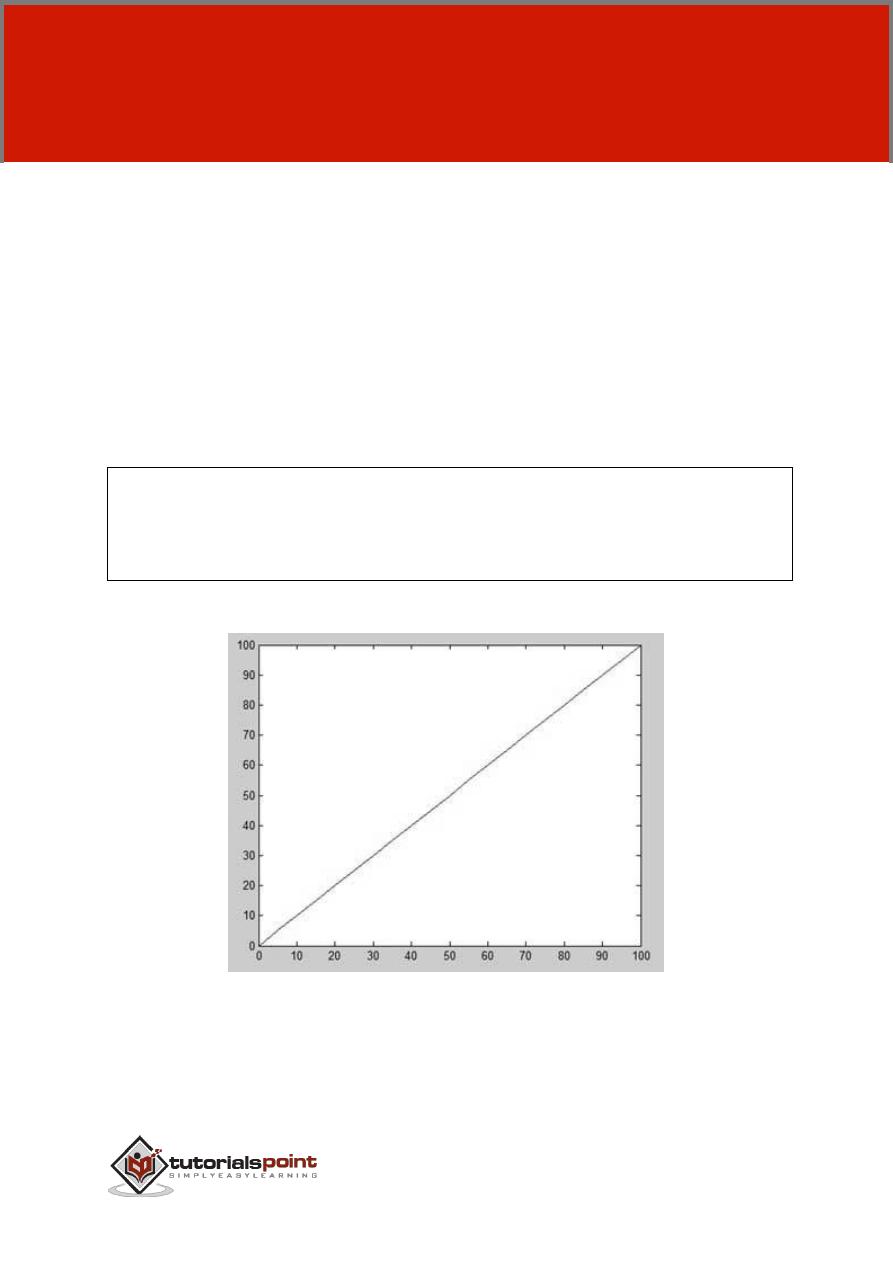
156
To plot the graph of a function, you need to take the following steps:
Define
x, by specifying the
range of values
for the variable
x, for which the
function is to be plotted
Define the function,
y = f(x)
Call the
plot
command, as
plot(x, y)
Following example would demonstrate the concept. Let us plot the simple
function
y = x
for the range of values for x from 0 to 100, with an increment of 5.
Create a script file and type the following code:
x = [0:5:100];
y = x;
plot(x, y)
When you run the file, MATLAB displays the following plot:
Let us take one more example to plot the function y = x
2
. In this example, we will
draw two graphs with the same function, but in second time, we will reduce the
value of increment. Please note that as we decrease the increment, the graph
becomes smoother.
20.
PLOTTING
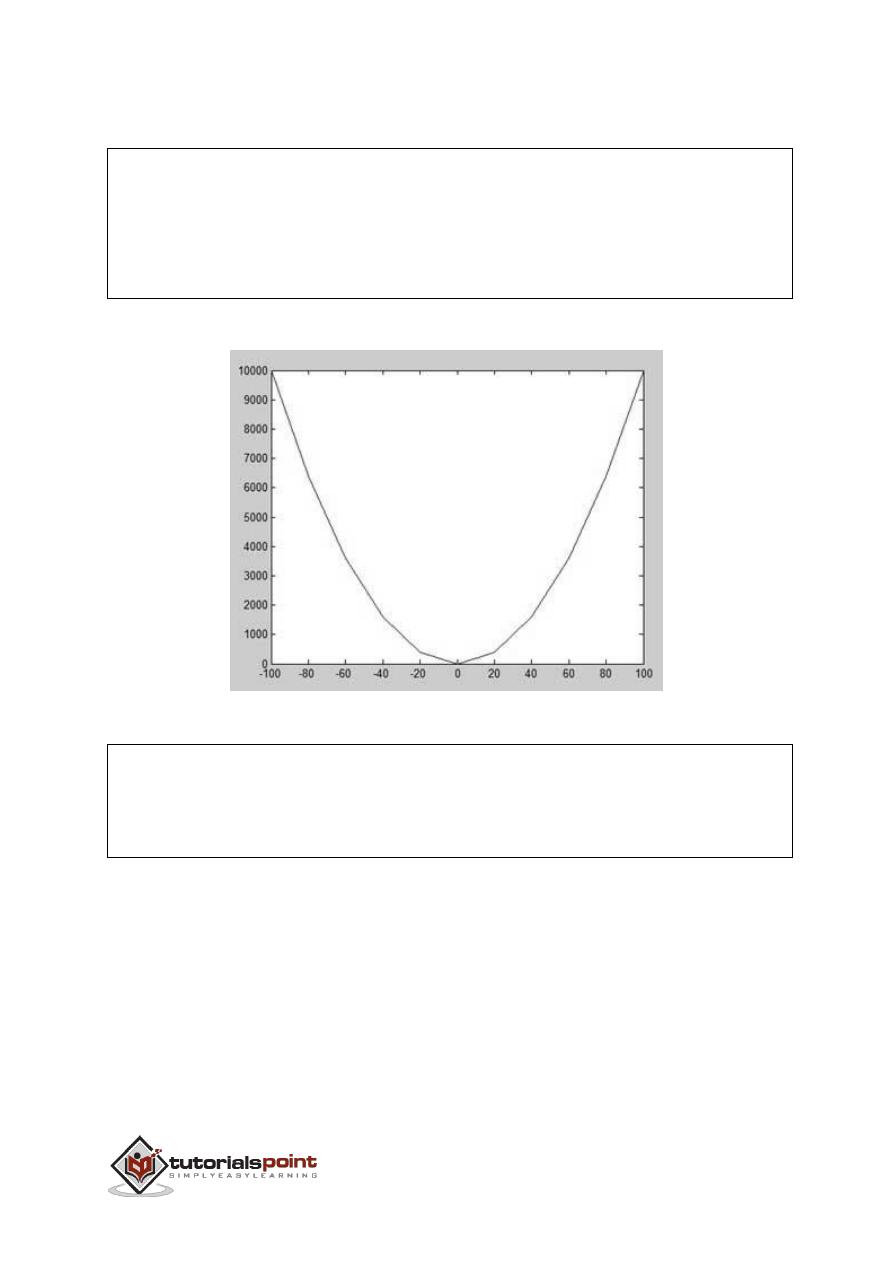
157
Create a script file and type the following code:
x
=
[1
2
3
4
5
6
7
8
9
10];
x
=
[-100:20:100];
y
=
x
.^2;
plot
(
x
,
y
)
When you run the file, MATLAB displays the following plot:
Change the code file a little, reduce the increment to 5:
x
=
[-100:5:100];
y
=
x
.^2;
plot
(
x
,
y
)

158
MATLAB draws a smoother graph:
Adding Title, Labels, Grid Lines, and Scaling on the Graph
MATLAB allows you to add title, labels along the x-axis and y-axis, grid lines and
also to adjust the axes to spruce up the graph.
The
xlabel
and
ylabel
commands generate labels along x-axis and y-axis.
The
title
command allows you to put a title on the graph.
The
grid on
command allows you to put the grid lines on the graph.
The
axis equal
command allows generating the plot with the same scale factors
and the spaces on both axes.
The
axis square
command generates a square plot.
Example
Create a script file and type the following code:
x
=
[0:0.01:10];
y
=
sin
(
x
);
plot
(
x
,
y
),
xlabel
('x'),
ylabel
('Sin(x)'),
title
('Sin(x) Graph'),
grid on
,
axis equal
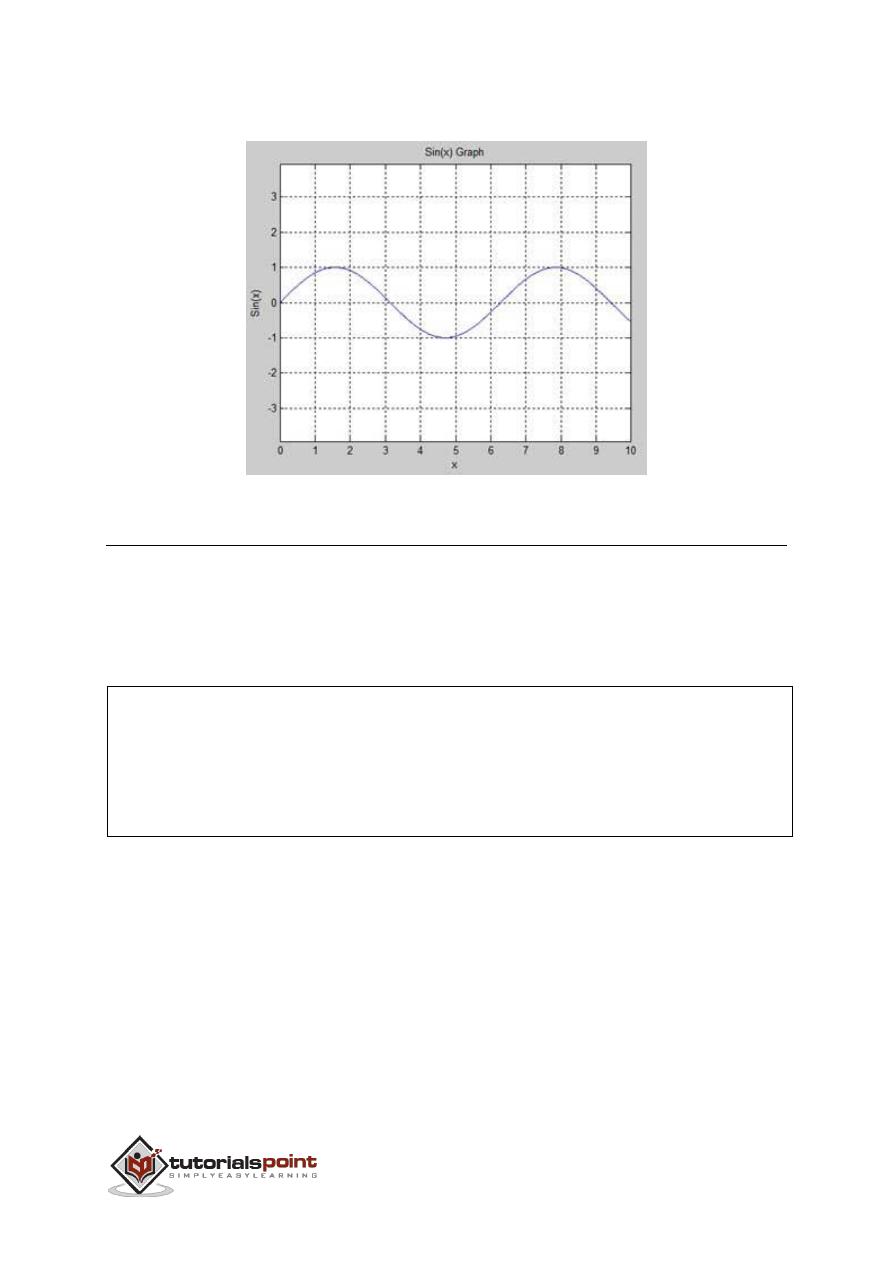
159
MATLAB generates the following graph:
Drawing Multiple Functions on the Same Graph
You can draw multiple graphs on the same plot. The following example
demonstrates the concept:
Example
Create a script file and type the following code:
x
=
[0
:
0.01:
10];
y
=
sin
(
x
);
g
=
cos
(
x
);
plot
(
x
,
y
,
x
,
g
,
'.-'),
legend
('Sin(x)',
'Cos(x)')
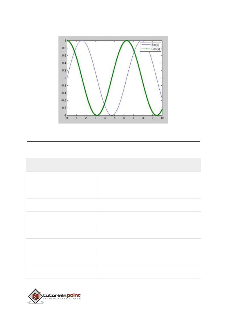
160
MATLAB generates the following graph:
Setting Colors on Graph
MATLAB provides eight basic color options for drawing graphs. The following table
shows the colors and their codes:
Code
Color
w
White
k
Black
b
Blue
r
Red
c
Cyan
g
Green
m
Magenta
y
Yellow
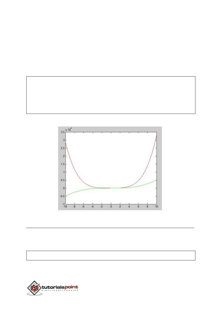
161
Example
Let us draw the graph of two polynomials
f(x) = 3x
4
+ 2x
3
+ 7x
2
+ 2x + 9 and
g(x) = 5x
3
+ 9x + 2
Create a script file and type the following code:
x
=
[-10
:
0.01:
10];
y
=
3*
x
.^4
+
2
*
x
.^3
+
7
*
x
.^2
+
2
*
x
+
9;
g
=
5
*
x
.^3
+
9
*
x
+
2;
plot
(
x
,
y
,
'r',
x
,
g
,
'g')
When you run the file, MATLAB generates the following graph:
Setting Axis Scales
The axis command allows you to set the axis scales. You can provide minimum
and maximum values for x and y axes using the axis command in the following
way:
axis ( [xmin xmax ymin ymax] )
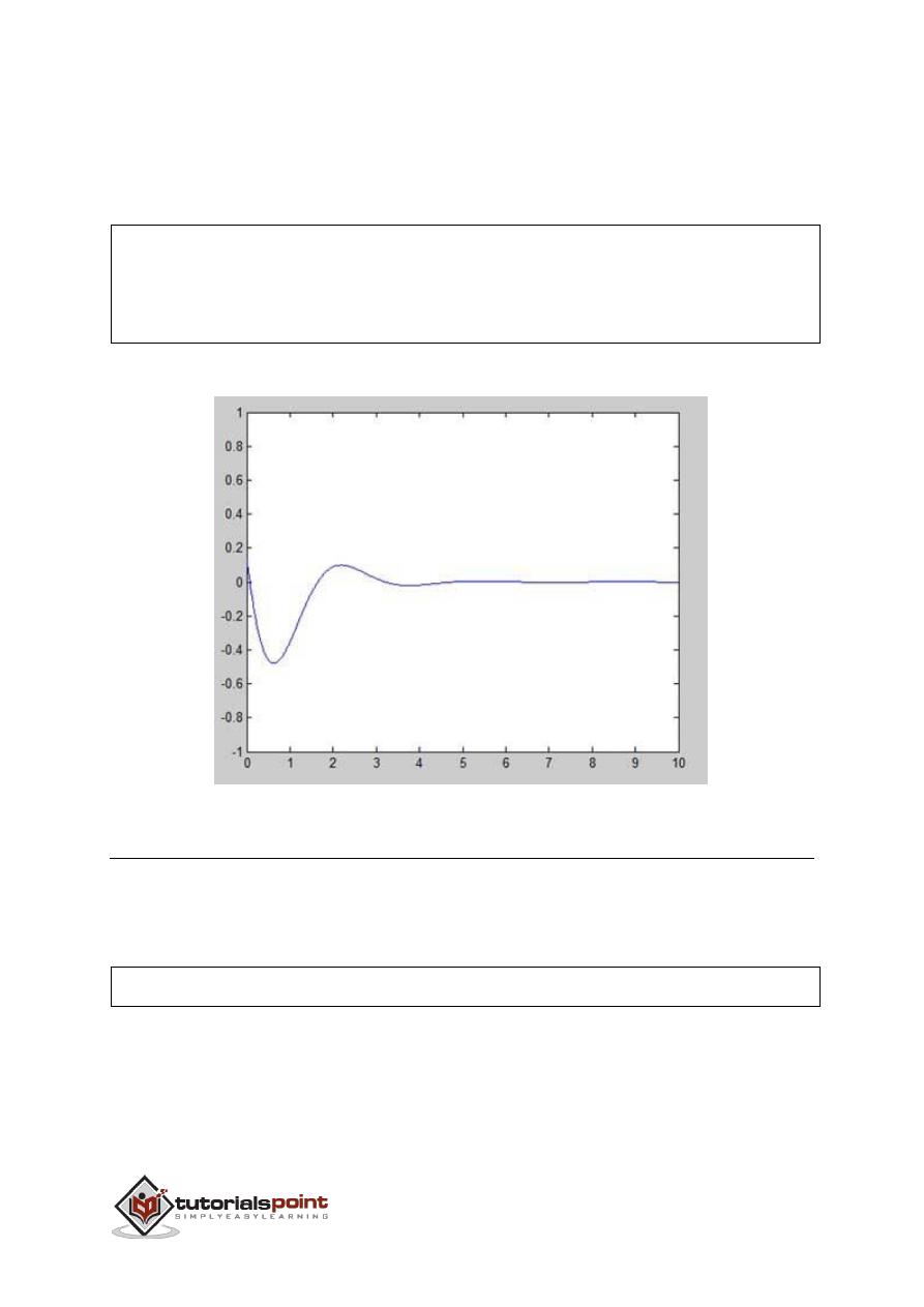
162
The following example shows this:
Example
Create a script file and type the following code:
x
=
[0
:
0.01:
10];
y
=
exp
(-
x
).*
sin
(2*
x
+
3);
plot
(
x
,
y
),
axis
([0
10
-1
1])
When you run the file, MATLAB generates the following graph:
Generating Sub-Plots
When you create an array of plots in the same figure, each of these plots is called
a subplot. The
subplot
command is used for creating subplots.
Syntax for the command is:
subplot(m, n, p)
where,
m
and
n
are the number of rows and columns of the plot array
and
p
specifies where to put a particular plot.
Each plot created with the subplot command can have its own characteristics.
Following example demonstrates the concept:
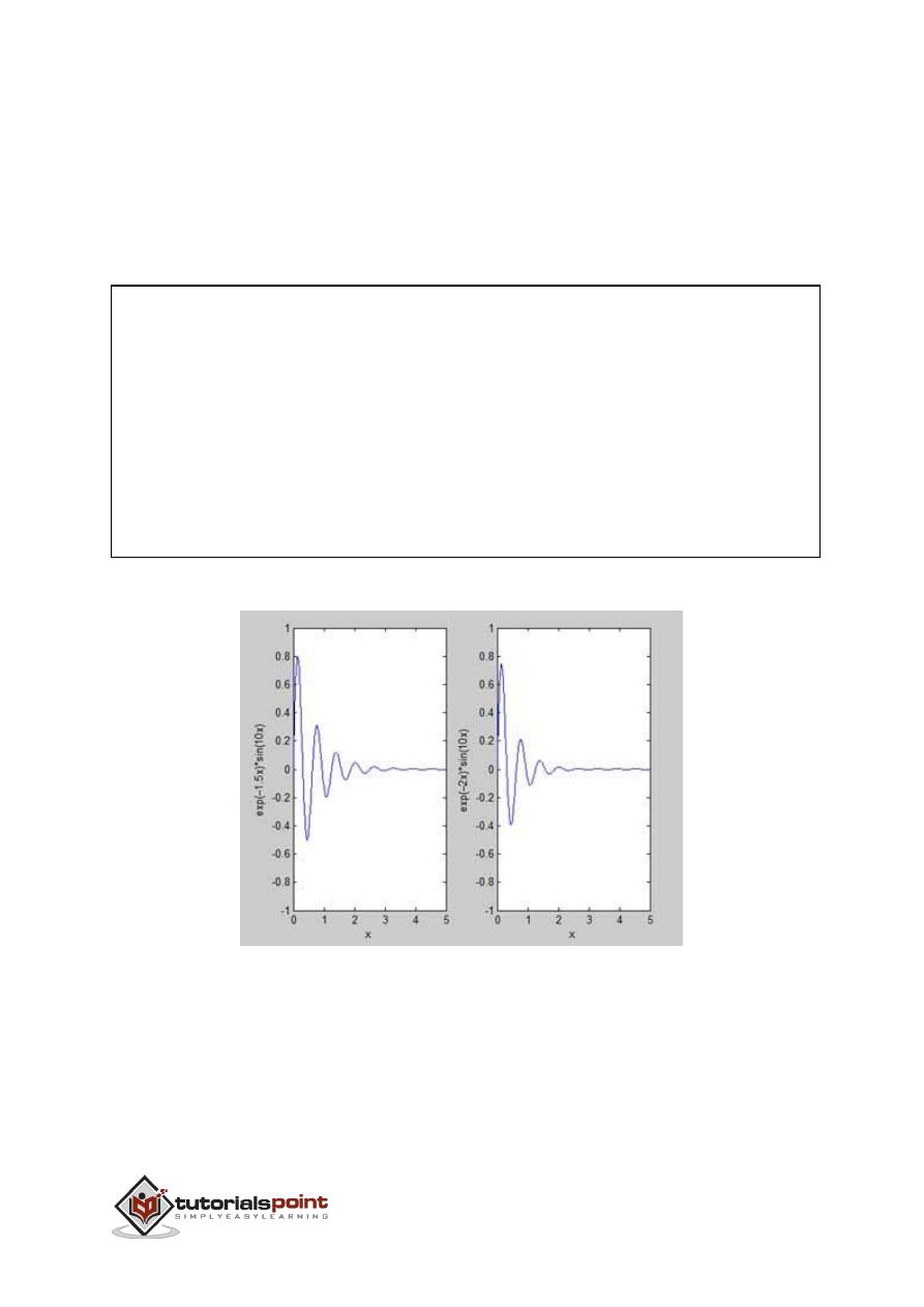
163
Example
Let us generate two plots:
y = e
−1.5x
sin(10x)
y = e
−2x
sin(10x)
Create a script file and type the following code:
x
=
[0:0.01:5];
y
=
exp
(-1.5*
x
).*
sin
(10*
x
);
subplot
(1,2,1)
plot
(
x
,
y
),
xlabel
('x'),
ylabel
('exp(–1.5x)*sin(10x)'),
axis
([0
5
-1
1])
y
=
exp
(-2*
x
).*
sin
(10*
x
);
subplot
(1,2,2)
plot
(
x
,
y
),
xlabel
('x'),
ylabel
('exp(–2x)*sin(10x)'),
axis
([0
5
-1
1])
When you run the file, MATLAB generates the following graph:

164
This chapter will continue exploring the plotting and graphics capabilities of
MATLAB. We will discuss:
Drawing bar charts
Drawing contours
Three dimensional plots
Drawing Bar Charts
The
bar
command draws a two dimensional bar chart. Let us take up an example
to demonstrate the idea.
Example
Let us have an imaginary classroom with 10 students. We know the percent of
marks obtained by these students are 75, 58, 90, 87, 50, 85, 92, 75, 60 and 95.
We will draw the bar chart for this data.
Create a script file and type the following code:
x
=
[1:10];
y
=
[75,
58,
90,
87,
50,
85,
92,
75,
60,
95];
bar
(
x
,
y
),
xlabel
('Student'),
ylabel
('Score'),
title
('First Sem:')
-
deps graph
.
eps
21.
GRAPHICS
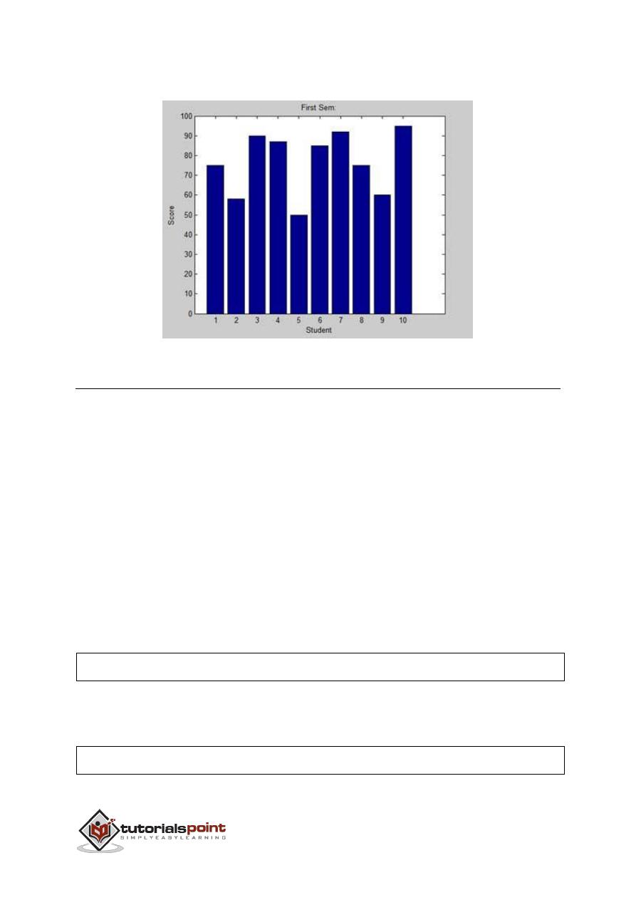
165
When you run the file, MATLAB displays the following bar chart:
Drawing Contours
A contour line of a function of two variables is a curve along which the function
has a constant value. Contour lines are used for creating contour maps by joining
points of equal elevation above a given level, such as mean sea level.
MATLAB provides a
contour
function for drawing contour maps.
Example
Let us generate a contour map that shows the contour lines for a given function g
= f(x, y). This function has two variables. So, we will have to generate two
independent variables, i.e., two data sets x and y. This is done by calling
the
meshgrid
command.
The
meshgrid
command is used for generating a matrix of elements that give the
range over x and y along with the specification of increment in each case.
Let us plot our function g = f(x, y), where −5 ≤ x ≤ 5, −3 ≤ y ≤ 3. Let us take an
increment of 0.1 for both the values. The variables are set as:
[x,y] = meshgrid(–5:0.1:5, –3:0.1:3);
Lastly, we need to assign the function. Let our function be: x
2
+ y
2
Create a script file and type the following code:
[x,y] = meshgrid(-5:0.1:5,-3:0.1:3); %independent variables
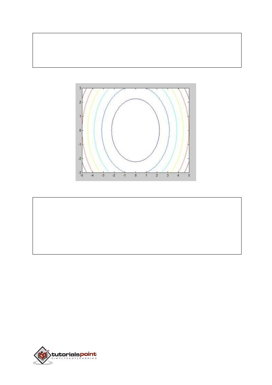
166
g = x.^2 + y.^2; % our function
contour(x,y,g) % call the contour function
print -deps graph.eps
When you run the file, MATLAB displays the following contour map:
Let us modify the code a little to spruce up the map:
[x,y] = meshgrid(-5:0.1:5,-3:0.1:3); %independent variables
g = x.^2 + y.^2; % our function
[C, h] = contour(x,y,g); % call the contour function
set(h,'ShowText','on','TextStep',get(h,'LevelStep')*2)
print -deps graph.eps
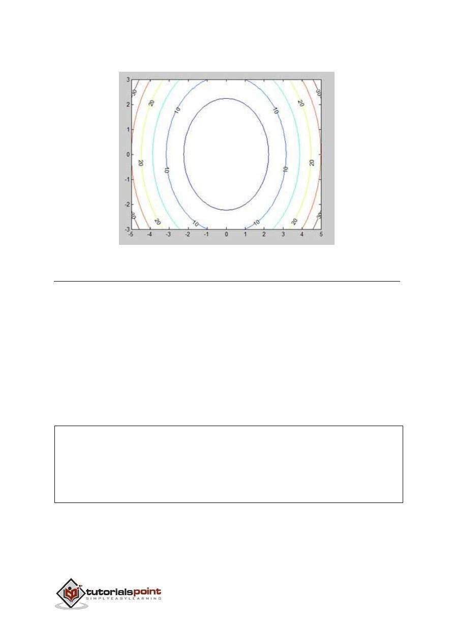
167
When you run the file, MATLAB displays the following contour map:
Three-Dimensional Plots
Three-dimensional plots basically display a surface defined by a function in two
variables, g = f (x,y).
As before, to define g, we first create a set of (x,y) points over the domain of the
function using the
meshgrid
command. Next, we assign the function itself. Finally,
we use the
surf command to create a surface plot.
The following example demonstrates the concept:
Example
Let us create a 3D surface map for the function g = xe
-(x2 + y2)
Create a script file and type the following code:
[x,y] = meshgrid(-2:.2:2);
g = x .* exp(-x.^2 - y.^2);
surf(x, y, g)
print -deps graph.eps
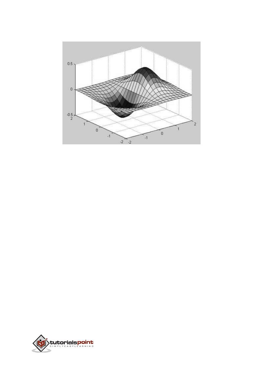
168
When you run the file, MATLAB displays the following 3-D map:
You can also use the
mesh
command to generate a three-dimensional surface.
However, the
surf
command displays both the connecting lines and the faces of
the surface in color, whereas, the
mesh
command creates a wireframe surface
with colored lines connecting the defining points.

169
So far, we have seen that all the examples work in MATLAB as well as its GNU,
alternatively called Octave. But for solving basic algebraic equations, both MATLAB
and Octave are little different, so we will try to cover MATLAB and Octave in
separate sections.
We will also discuss factorizing and simplification of algebraic expressions.
Solving Basic Algebraic Equations in MATLAB
The
solve
function is used for solving algebraic equations. In its simplest form,
the solve function takes the equation enclosed in quotes as an argument.
For example, let us solve for x in the equation x-5 = 0
solve('x-5=0')
MATLAB will execute the above statement and return the following result:
ans =
5
You can also call the solve function as:
y = solve('x-5 = 0')
MATLAB will execute the above statement and return the following result:
y =
5
You may even not include the right hand side of the equation:
solve('x-5')
MATLAB will execute the above statement and return the following result:
ans =
22.
ALGEBRA

170
5
If the equation involves multiple symbols, then MATLAB by default assumes that
you are solving for x, however, the solve command has another form:
solve(equation, variable)
where, you can also mention the variable.
For example, let us solve the equation v – u – 3t
2
= 0, for v. In this case, we
should write:
solve('v-u-3*t^2=0', 'v')
MATLAB will execute the above statement and return the following result:
ans =
3*t^2 + u
Solving Basic Algebraic Equations in Octave
The
roots
command is used for solving algebraic equations in Octave and you can
write above examples as follows:
For example, let us solve for x in the equation x-5 = 0
roots([1, -5])
Octave will execute the above statement and return the following result:
ans =
5
You can also call the solve function as:
y = roots([1, -5])
Octave will execute the above statement and return the following result:

171
y =
5
Solving Quadratic Equations in MATLAB
The
solve
function can also solve higher order equations. It is often used to solve
quadratic equations. The function returns the roots of the equation in an array.
The following example solves the quadratic equation x
2
-7x +12 = 0. Create a
script file and type the following code:
eq = 'x^2 -7*x + 12 = 0';
s = solve(eq);
disp('The first root is: '), disp(s(1));
disp('The second root is: '), disp(s(2));
When you run the file, it displays the following result:
The first root is:
3
The second root is:
4
Solving Quadratic Equations in Octave
The following example solves the quadratic equation x
2
-7x +12 = 0 in Octave.
Create a script file and type the following code:
s = roots([1, -7, 12]);
disp('The first root is: '), disp(s(1));
disp('The second root is: '), disp(s(2));
When you run the file, it displays the following result:

172
The first root is:
4
The second root is:
3
Solving Higher Order Equations in MATLAB
The
solve
command can also solve higher order equations. For example, let us
solve a cubic equation as (x-3)
2
(x-7) = 0
solve('(x-3)^2*(x-7)=0')
MATLAB will execute the above statement and return the following result:
ans =
3
3
7
In case of higher order equations, roots are long containing many terms. You can
get the numerical value of such roots by converting them to double. The following
example solves the fourth order equation x
4
− 7x
3
+ 3x
2
− 5x + 9 = 0.
Create a script file and type the following code:
eq = 'x^4 - 7*x^3 + 3*x^2 - 5*x + 9 = 0';
s = solve(eq);
disp('The first root is: '), disp(s(1));
disp('The second root is: '), disp(s(2));
disp('The third root is: '), disp(s(3));
disp('The fourth root is: '), disp(s(4));
% converting the roots to double type
disp('Numeric value of first root'), disp(double(s(1)));

173
disp('Numeric value of second root'), disp(double(s(2)));
disp('Numeric value of third root'), disp(double(s(3)));
disp('Numeric value of fourth root'), disp(double(s(4)));
When you run the file, it returns the following result:
The first root is:
6.630396332390718431485053218985
The second root is:
1.0597804633025896291682772499885
The third root is:
- 0.34508839784665403032666523448675 -
1.0778362954630176596831109269793*i
The fourth root is:
- 0.34508839784665403032666523448675 +
1.0778362954630176596831109269793*i
Numeric value of first root
6.6304
Numeric value of second root
1.0598
Numeric value of third root
-0.3451 - 1.0778i
Numeric value of fourth root
-0.3451 + 1.0778i
Please note that the last two roots are complex numbers.

174
Solving Higher Order Equations in Octave
The following example solves the fourth order equation x
4
− 7x
3
+ 3x
2
− 5x + 9 =
0.
Create a script file and type the following code:
v = [1, -7, 3, -5, 9];
s = roots(v);
% converting the roots to double type
disp('Numeric value of first root'), disp(double(s(1)));
disp('Numeric value of second root'), disp(double(s(2)));
disp('Numeric value of third root'), disp(double(s(3)));
disp('Numeric value of fourth root'), disp(double(s(4)));
When you run the file, it returns the following result:
Numeric value of first root
6.6304
Numeric value of second root
-0.34509 + 1.07784i
Numeric value of third root
-0.34509 - 1.07784i
Numeric value of fourth root
1.0598
Solving System of Equations in MATLAB
The
solve
function can also be used to generate solutions of systems of equations
involving more than one variables. Let us take up a simple example to
demonstrate this use.
Let us solve the equations:

175
5x + 9y = 5
3x – 6y = 4
Create a script file and type the following code:
s
=
solve
('5*x + 9*y = 5','3*x - 6*y = 4');
s
.
x
s
.
y
When you run the file, it displays the following result:
ans
=
22/19
ans
=
-5/57
In same way, you can solve larger linear systems. Consider the following set of
equations:
x + 3y -2z = 5
3x + 5y + 6z = 7
2x + 4y + 3z = 8
Solving System of Equations in Octave
We have a little different approach to solve a system of 'n' linear equations in 'n'
unknowns. Let us take up a simple example to demonstrate this use.
Let us solve the equations:
5x + 9y = 5
3x – 6y = 4
Such a system of linear equations can be written as the single matrix equation Ax
= b, where A is the coefficient matrix, b is the column vector containing the right-
hand side of the linear equations and x is the column vector representing the
solution as shown in the below program:
Create a script file and type the following code:

176
A = [5, 9; 3, -6];
b = [5;4];
A \ b
When you run the file, it displays the following result:
ans =
1.157895
-0.087719
In same way, you can solve larger linear systems as given below:
x + 3y -2z = 5
3x + 5y + 6z = 7
2x + 4y + 3z = 8
Expanding and Collecting Equations in MATLAB
The
expand
and the
collect
commands expands and collects an equation
respectively. The following example demonstrates the concepts:
When you work with many symbolic functions, you should declare that your
variables are symbolic.
Create a script file and type the following code:
syms x %symbolic variable x
syms y %symbolic variable x
% expanding equations
expand((x-5)*(x+9))
expand((x+2)*(x-3)*(x-5)*(x+7))
expand(sin(2*x))
expand(cos(x+y))

177
% collecting equations
collect(x^3 *(x-7))
collect(x^4*(x-3)*(x-5))
When you run the file, it displays the following result:
ans =
x^2 + 4*x - 45
ans =
x^4 + x^3 - 43*x^2 + 23*x + 210
ans =
2*cos(x)*sin(x)
ans =
cos(x)*cos(y) - sin(x)*sin(y)
ans =
x^4 - 7*x^3
ans =
x^6 - 8*x^5 + 15*x^4
Expanding and Collecting Equations in Octave
You need to have
symbolic
package, which provides
expand
and
collect
command to expand and collect an equation, respectively. The following
example demonstrates the concepts:
When you work with many symbolic functions, you should declare that your
variables are symbolic but Octave has different approach to define symbolic
variables. Notice the use of Sin
and
Cos which are also defined in symbolic
package.
Create a script file and type the following code:
% first of all load the package, make sure it’s installed.

178
pkg load symbolic
% make symbols module available
symbols
% define symbolic variables
x = sym ('x');
y = sym ('y');
z = sym ('z');
% expanding equations
expand((x-5)*(x+9))
expand((x+2)*(x-3)*(x-5)*(x+7))
expand(Sin(2*x))
expand(Cos(x+y))
% collecting equations
collect(x^3 *(x-7), z)
collect(x^4*(x-3)*(x-5), z)
When you run the file, it displays the following result:
ans =
-45.0+x^2+(4.0)*x
ans =
210.0+x^4-(43.0)*x^2+x^3+(23.0)*x

179
ans =
sin((2.0)*x)
ans =
cos(y+x)
ans =
x^(3.0)*(-7.0+x)
ans =
(-3.0+x)*x^(4.0)*(-5.0+x)
Factorization and Simplification of Algebraic Expressions
The
factor
function factorizes an expression and the
simplify
function simplifies
an expression. The following example demonstrates the concept:
Example
Create a script file and type the following code:
syms x
syms y
factor(x^3 - y^3)
factor([x^2-y^2,x^3+y^3])
simplify((x^4-16)/(x^2-4))
When you run the file, it displays the following result:
ans =
(x - y)*(x^2 + x*y + y^2)

180
ans =
[ (x - y)*(x + y), (x + y)*(x^2 - x*y + y^2)]
ans =
x^2 + 4

181
MATLAB provides various ways for solving problems of differential and integral
calculus, solving differential equations of any degree and calculation of limits. Best
of all, you can easily plot the graphs of complex functions and check maxima,
minima and other stationery points on a graph by solving the original function, as
well as its derivative.
This chapter will deal with problems of calculus.. In this chapter, we will discuss
pre-calculus concepts i.e., calculating limits of functions and verifying the
properties of limits.
In the next chapter
Differential, we will compute derivative of an expression and
find the local maxima and minima on a graph. We will also discuss solving
differential equations.
Finally, in the
Integration
chapter, we will discuss integral calculus.
Calculating Limits
MATLAB provides the
limit
command for calculating limits. In its most basic form,
the
limit command takes expression as an argument and finds the limit of the
expression as the independent variable goes to zero.
For example, let us calculate the limit of a function f(x) = (x
3
+ 5)/(x
4
+ 7), as x
tends to zero.
syms x
limit((x^3 + 5)/(x^4 + 7))
MATLAB will execute the above statement and return the following result:
ans =
5/7
The limit function falls in the realm of symbolic computing; you need to use
the
syms function to tell MATLAB which symbolic variables you are using. You can
also compute limit of a function, as the variable tends to some number other than
zero. To calculate lim
x->a
(f(x)), we use the limit command with arguments. The
first being the expression and the second is the number, that
x
approaches, here
it is
a.
23.
CALCULUS

182
For example, let us calculate limit of a function f(x) = (x-3)/(x-1), as x tends to
1.
limit((x - 3)/(x-1),1)
MATLAB will execute the above statement and return the following result:
ans =
NaN
Let's take another example,
limit(x^2 + 5, 3)
MATLAB will execute the above statement and return the following result:
ans =
14
Calculating Limits using Octave
Following is Octave version of the above example using
symbolic
package, try to
execute and compare the result:
pkg load symbolic
symbols
x=sym("x");
subs((x^3+5)/(x^4+7),x,0)
Octave will execute the above statement and return the following result:
ans =
0.7142857142857142857
Verification of Basic Properties of Limits

183
Algebraic Limit Theorem provides some basic properties of limits. These are as
follows:
Let us consider two functions:
f(x) = (3x + 5)/(x - 3)
g(x) = x
2
+ 1.
Let us calculate the limits of the functions as x tends to 5, of both functions and
verify the basic properties of limits using these two functions and MATLAB.
Example
Create a script file and type the following code into it:
syms x
f = (3*x + 5)/(x-3);
g = x^2 + 1;
l1 = limit(f, 4)
l2 = limit (g, 4)
lAdd = limit(f + g, 4)
lSub = limit(f - g, 4)
lMult = limit(f*g, 4)
lDiv = limit (f/g, 4)
When you run the file, it displays:
l1 =
17
l2 =

184
17
lAdd =
34
lSub =
0
lMult =
289
lDiv =
1
Verification of Basic Properties of Limits using Octave
Following is Octave version of the above example using
symbolic
package, try to
execute and compare the result:
pkg load symbolic
symbols
x = sym("x");
f = (3*x + 5)/(x-3);
g = x^2 + 1;
l1=subs(f, x, 4)
l2 = subs (g, x, 4)
lAdd = subs (f+g, x, 4)

185
lSub = subs (f-g, x, 4)
lMult = subs (f*g, x, 4)
lDiv = subs (f/g, x, 4)
Octave will execute the above statement and return the following result:
l1 =
17.0
l2 =
17.0
lAdd =
34.0
lSub =
0.0
lMult =
289.0
lDiv =
1.0
Left and Right Sided Limits
When a function has a discontinuity for some particular value of the variable, the
limit does not exist at that point. In other words, limits of a function f(x) has

186
discontinuity at x = a, when the value of limit, as x approaches x from left side,
does not equal the value of the limit as x approaches from right side.
This leads to the concept of left-handed and right-handed limits. A left-handed
limit is defined as the limit as x -> a, from the left, i.e., x approaches a, for values
of x < a. A right-handed limit is defined as the limit as x -> a, from the right, i.e.,
x approaches a, for values of x > a. When the left-handed limit and right-handed
limit are not equal, the limit does not exist.
Let us consider a function:
f(x) = (x - 3)/|x - 3|
We will show that lim
x->3
f(x) does not exist. MATLAB helps us to establish this fact
in two ways:
By plotting the graph of the function and showing the discontinuity
By computing the limits and showing that both are different.
The left-handed and right-handed limits are computed by passing the character
strings 'left' and 'right' to the limit command as the last argument.
Example
Create a script file and type the following code into it:
f = (x - 3)/abs(x-3);
ezplot(f,[-1,5])
l = limit(f,x,3,'left')
r = limit(f,x,3,'right')
When you run the file, MATLAB draws the following plot,
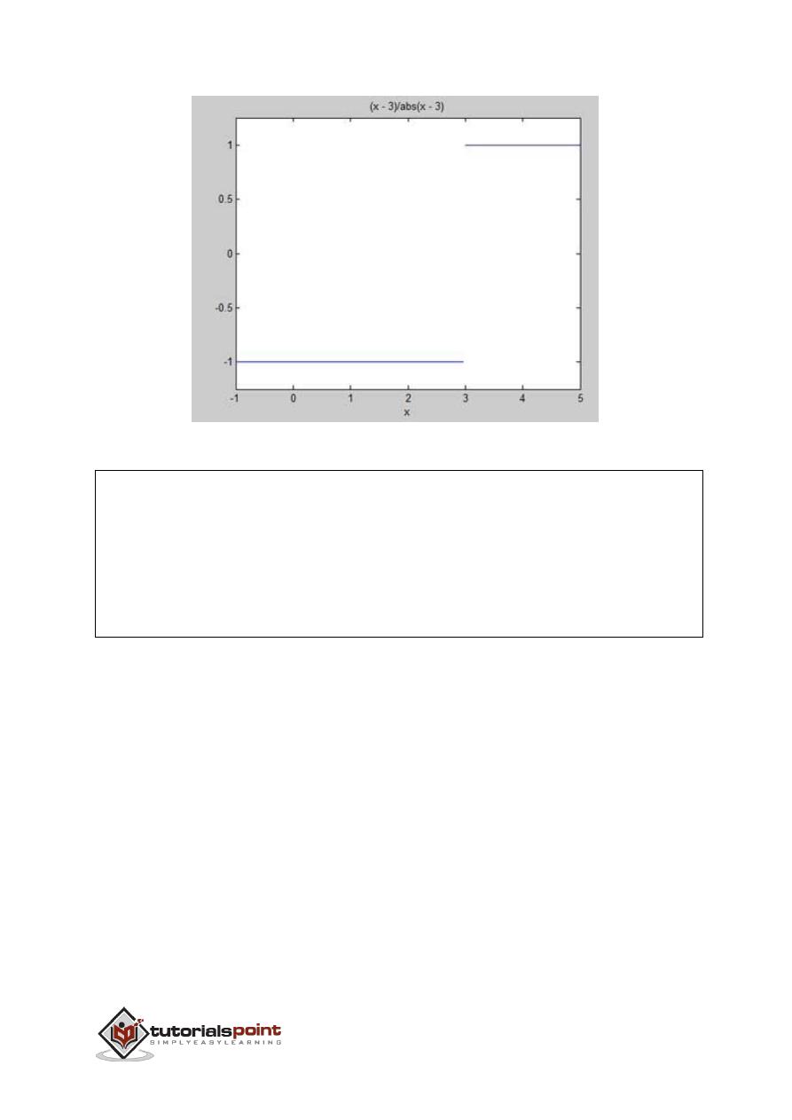
187
and displays the following output:
l =
-1
r =
1

188
MATLAB provides the
diff
command for computing symbolic derivatives. In its
simplest form, you pass the function you want to differentiate to diff command as
an argument.
For example, let us compute the derivative of the function f(t) = 3t
2
+ 2t
-2
Example
Create a script file and type the following code into it:
syms t
f = 3*t^2 + 2*t^(-2);
diff(f)
When the above code is compiled and executed, it produces the following result:
ans =
6*t - 4/t^3
Following is Octave equivalent of the above calculation:
pkg load symbolic
symbols
t = sym("t");
f = 3*t^2 + 2*t^(-2);
differentiate(f,t)
24.
DIFFERENTIAL

189
Octave executes the code and returns the following result:
ans =
-(4.0)*t^(-3.0)+(6.0)*t
Verification of Elementary Rules of Differentiation
Let us briefly state various equations or rules for differentiation of functions and
verify these rules. For this purpose, we will write f'(x) for a first order derivative
and f"(x) for a second order derivative.
Following are the rules for differentiation:
Rule 1
For any functions f and g and any real numbers a and b are the derivative of the
function:
h(x) = af(x) + bg(x)
with respect to x is given by:
h'(x) = af'(x) + bg'(x)
Rule 2
The
sum
and
subtraction
rules state that if f and g are two functions, f' and g'
are their derivatives respectively, then,
(f + g)' = f' + g'
(f - g)' = f' - g'
Rule 3
The
product
rule states that if f and g are two functions, f' and g' are their
derivatives respectively, then,
(f.g)' = f'.g + g'.f
Rule 4
The
quotient
rule states that if f and g are two functions, f' and g' are their
derivatives respectively, then,
(f/g)' = (f'.g - g'.f)/g
2
Rule 5
The
polynomial
or elementary power rule states that, if
y = f(x) = x
n
, then
f' =
n. x
(n-1)

190
A direct outcome of this rule is that the derivative of any constant is zero, i.e., if
y
= k, any constant, then
f' = 0
Rule 6
The
chain
rule states that, the derivative of the function of a function
h(x) =
f(g(x))
with respect to x is,
h'(x)= f'(g(x)).g'(x)
Example
Create a script file and type the following code into it:
syms x
syms t
f = (x + 2)*(x^2 + 3)
der1 = diff(f)
f = (t^2 + 3)*(sqrt(t) + t^3)
der2 = diff(f)
f = (x^2 - 2*x + 1)*(3*x^3 - 5*x^2 + 2)
der3 = diff(f)
f = (2*x^2 + 3*x)/(x^3 + 1)
der4 = diff(f)
f = (x^2 + 1)^17
der5 = diff(f)
f = (t^3 + 3* t^2 + 5*t -9)^(-6)
der6 = diff(f)
When you run the file, MATLAB displays the following result:
f =
(x^2 + 3)*(x + 2)

191
der1 =
2*x*(x + 2) + x^2 + 3
f =
(t^(1/2) + t^3)*(t^2 + 3)
der2 =
(t^2 + 3)*(3*t^2 + 1/(2*t^(1/2))) + 2*t*(t^(1/2) + t^3)
f =
(x^2 - 2*x + 1)*(3*x^3 - 5*x^2 + 2)
der3 =
(2*x - 2)*(3*x^3 - 5*x^2 + 2) - (- 9*x^2 + 10*x)*(x^2 - 2*x + 1)
f =
(2*x^2 + 3*x)/(x^3 + 1)
der4 =
(4*x + 3)/(x^3 + 1) - (3*x^2*(2*x^2 + 3*x))/(x^3 + 1)^2
f =
(x^2 + 1)^17
der5 =
34*x*(x^2 + 1)^16

192
f =
1/(t^3 + 3*t^2 + 5*t - 9)^6
der6 =
-(6*(3*t^2 + 6*t + 5))/(t^3 + 3*t^2 + 5*t - 9)^7
Following is Octave equivalent of the above calculation:
pkg load symbolic
symbols
x=sym("x");
t=sym("t");
f = (x + 2)*(x^2 + 3)
der1 = differentiate(f,x)
f = (t^2 + 3)*(t^(1/2) + t^3)
der2 = differentiate(f,t)
f = (x^2 - 2*x + 1)*(3*x^3 - 5*x^2 + 2)
der3 = differentiate(f,x)
f = (2*x^2 + 3*x)/(x^3 + 1)
der4 = differentiate(f,x)
f = (x^2 + 1)^17
der5 = differentiate(f,x)
f = (t^3 + 3* t^2 + 5*t -9)^(-6)
der6 = differentiate(f,t)

193
Derivatives of Exponential, Logarithmic, and Trigonometric
Functions
The following table provides the derivatives of commonly used exponential,
logarithmic and trigonometric functions:
Function
Derivative
c
a.x
c
a.x
.ln c.a (ln is natural logarithm)
e
x
e
x
ln x
1/x
ln
c
x
1/x.ln c
x
x
x
x
.(1 + ln x)
sin(x)
cos(x)
cos(x)
-sin(x)
tan(x)
sec
2
(x), or 1/cos
2
(x), or 1 + tan
2
(x)
cot(x)
-csc
2
(x), or -1/sin
2
(x), or -(1 + cot
2
(x))
sec(x)
sec(x).tan(x)
csc(x)
-csc(x).cot(x)
Example
Create a script file and type the following code into it:
syms x
y = exp(x)
diff(y)
y = x^9

194
diff(y)
y = sin(x)
diff(y)
y = tan(x)
diff(y)
y = cos(x)
diff(y)
y = log(x)
diff(y)
y = log10(x)
diff(y)
y = sin(x)^2
diff(y)
y = cos(3*x^2 + 2*x + 1)
diff(y)
y = exp(x)/sin(x)
diff(y)
When you run the file, MATLAB displays the following result:
y
=
exp(x)
ans =
exp(x)
y =
x^9

195
ans =
9*x^8
y =
sin(x)
ans =
cos(x)
y =
tan(x)
ans =
tan(x)^2 + 1
y =
cos(x)
ans =
-sin(x)
y =
log(x)
ans =
1/x
y =
log(x)/log(10)
ans =

196
1/(x*log(10))
y =
sin(x)^2
ans =
2*cos(x)*sin(x)
y =
cos(3*x^2 + 2*x + 1)
ans =
-sin(3*x^2 + 2*x + 1)*(6*x + 2)
y =
exp(x)/sin(x)
ans =
exp(x)/sin(x) - (exp(x)*cos(x))/sin(x)^2
Following is Octave equivalent of the above calculation:
pkg load symbolic
symbols
x = sym("x");
y = Exp(x)
differentiate(y,x)
y = x^9

197
differentiate(y,x)
y = Sin(x)
differentiate(y,x)
y = Tan(x)
differentiate(y,x)
y = Cos(x)
differentiate(y,x)
y = Log(x)
differentiate(y,x)
% symbolic packages does not have this support
%y = Log10(x)
%differentiate(y,x)
y = Sin(x)^2
differentiate(y,x)
y = Cos(3*x^2 + 2*x + 1)
differentiate(y,x)
y = Exp(x)/Sin(x)
differentiate(y,x)

198
Computing Higher Order Derivatives
To compute higher derivatives of a function f, we use the syntax
diff(f,n).
Let us compute the second derivative of the function y = f(x) = x .e
-3x
f = x*exp(-3*x);
diff(f, 2)
MATLAB executes the code and returns the following result:
ans =
9*x*exp(-3*x) - 6*exp(-3*x)
Following is Octave equivalent of the above calculation:
pkg load symbolic
symbols
x = sym("x");
f = x*Exp(-3*x);
differentiate(f, x, 2)
Example
In this example, let us solve a problem. Given that a function
y = f(x) = 3 sin(x)
+ 7 cos(5x). We will have to find out whether the equation
f" + f = -
5cos(2x)
holds true.
Create a script file and type the following code into it:
syms x
y = 3*sin(x)+7*cos(5*x); % defining the function
lhs = diff(y,2)+y; %evaluating the lhs of the equation

199
rhs = -5*cos(2*x); %rhs of the equation
if(isequal(lhs,rhs))
disp('Yes, the equation holds true');
else
disp('No, the equation does not hold true');
end
disp('Value of LHS is: '), disp(lhs);
When you run the file, it displays the following result:
No, the equation does not hold true
Value of LHS is:
-168*cos(5*x)
Following is Octave equivalent of the above calculation:
pkg load symbolic
symbols
x = sym("x");
y = 3*Sin(x)+7*Cos(5*x); % defining the function
lhs = differentiate(y, x, 2) + y; %evaluting the lhs of the equation
rhs = -5*Cos(2*x); %rhs of the equation
if(lhs == rhs)
disp('Yes, the equation holds true');
else
disp('No, the equation does not hold true');
end

200
disp('Value of LHS is: '), disp(lhs);
Finding the Maxima and Minima of a Curve
If we are searching for the local maxima and minima for a graph, we are basically
looking for the highest or lowest points on the graph of the function at a particular
locality, or for a particular range of values of the symbolic variable.
For a function y = f(x) the points on the graph where the graph has zero slope are
called stationary points. In other words stationary points are where f'(x) = 0.
To find the stationary points of a function we differentiate, we need to set the
derivative equal to zero and solve the equation.
Example
Let us find the stationary points of the function f(x) = 2x
3
+ 3x
2
− 12x + 17
Take the following steps:
First let us enter the function and plot its graph:
syms x
y = 2*x^3 + 3*x^2 - 12*x + 17; % defining the function
ezplot(y)
MATLAB executes the code and returns the following plot:
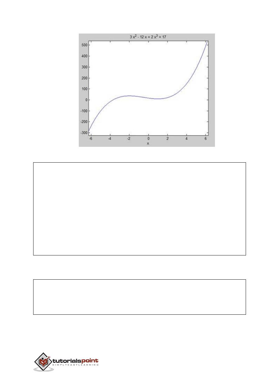
201
Here is Octave equivalent code for the above example:
pkg load symbolic
symbols
x = sym('x');
y = inline("2*x^3 + 3*x^2 - 12*x + 17");
ezplot(y)
print -deps graph.eps
Our aim is to find some local maxima and minima on the graph, so let us find the
local maxima and minima for the interval [-2, 2] on the graph.
syms x
y = 2*x^3 + 3*x^2 - 12*x + 17; % defining the function
ezplot(y, [-2, 2])
MATLAB executes the code and returns the following plot:
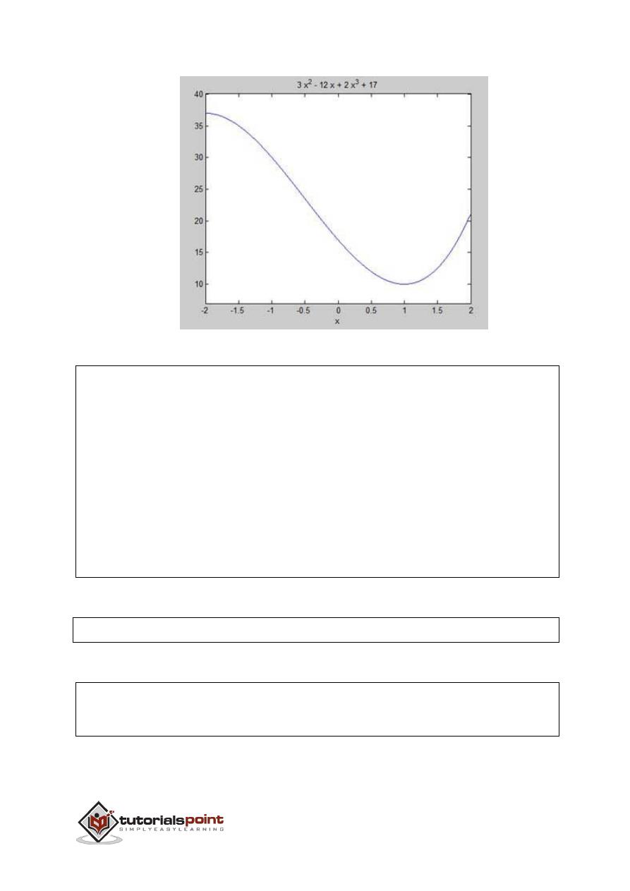
202
Here is Octave equivalent code for the above example:
pkg load symbolic
symbols
x = sym('x');
y = inline("2*x^3 + 3*x^2 - 12*x + 17");
ezplot(y, [-2, 2])
print -deps graph.eps
Next, let us compute the derivative
g = diff(y)
MATLAB executes the code and returns the following result:
g =
6*x^2 + 6*x - 12
Here is Octave equivalent of the above calculation:

203
pkg load symbolic
symbols
x = sym("x");
y = 2*x^3 + 3*x^2 - 12*x + 17;
g = differentiate(y,x)
Let us solve the derivative function, g, to get the values where it becomes zero.
s = solve(g)
MATLAB executes the code and returns the following result:
s =
1
-2
Following is Octave equivalent of the above calculation:
pkg load symbolic
symbols
x = sym("x");
y = 2*x^3 + 3*x^2 - 12*x + 17;
g = differentiate(y,x)
roots([6, 6, -12])
This agrees with our plot. So let us evaluate the function f at the critical points x
= 1, -2. We can substitute a value in a symbolic function by using the
subs
command.

204
subs(y, 1), subs(y, -2)
MATLAB executes the code and returns the following result:
ans =
10
ans =
37
Following is Octave equivalent of the above calculation:
pkg load symbolic
symbols
x = sym("x");
y = 2*x^3 + 3*x^2 - 12*x + 17;
g = differentiate(y,x)
roots([6, 6, -12])
subs(y, x, 1), subs(y, x, -2)
Therefore, The minimum and maximum values on the function f(x) = 2x
3
+ 3x
2
−
12x + 17, in the interval [-2,2] are 10 and 37.
Solving Differential Equations
MATLAB provides the
dsolve
command for solving differential equations
symbolically.
The most basic form of the
dsolve
command for finding the solution to a single
equation is:

205
dsolve('eqn')
where
eqn
is a text string used to enter the equation.
It returns a symbolic solution with a set of arbitrary constants that MATLAB labels
C1, C2, and so on.
You can also specify initial and boundary conditions for the problem, as comma-
delimited list following the equation as:
dsolve('eqn','cond1', 'cond2',…)
For the purpose of using dsolve command,
derivatives are indicated with a D.
For example, an equation like f'(t) = -2*f + cost(t) is entered as:
'Df = -2*f + cos(t)'
Higher derivatives are indicated by following D by the order of the derivative.
For example the equation f"(x) + 2f'(x) = 5sin3x should be entered as:
'D2y + 2Dy = 5*sin(3*x)'
Let us take up a simple example of a first order differential equation: y' = 5y.
s = dsolve('Dy = 5*y')
MATLAB executes the code and returns the following result:
s =
C2*exp(5*t)
Let us take up another example of a second order differential equation as: y" - y
= 0, y(0) = -1, y'(0) = 2.
dsolve('D2y - y = 0','y(0) = -1','Dy(0) = 2')
MATLAB executes the code and returns the following result:
ans =
exp(t)/2 - (3*exp(-t))/2

206
Integration deals with two essentially different types of problems.
In the first type, derivative of a function is given and we want to find the function.
Therefore, we basically reverse the process of differentiation. This reverse process
is known as anti-differentiation, or finding the primitive function, or finding an
indefinite integral.
The second type of problems involve adding up a very large number of very small
quantities and then taking a limit as the size of the quantities approaches zero,
while the number of terms tend to infinity. This process leads to the definition of
the
definite integral.
Definite integrals are used for finding area, volume, center of gravity, moment of
inertia, work done by a force, and in numerous other applications.
Finding Indefinite Integral Using MATLAB
By definition, if the derivative of a function f(x) is f'(x), then we say that an
indefinite integral of f'(x) with respect to x is f(x). For example, since the derivative
(with respect to x) of x
2
is 2x, we can say that an indefinite integral of 2x is x
2
.
In symbols:
f'(x
2
) = 2x, therefore,
∫ 2xdx = x
2
.
Indefinite integral is not unique, because derivative of x
2
+ c, for any value of a
constant c, will also be 2x.
This is expressed in symbols as:
∫ 2xdx = x
2
+ c.
Where, c is called an 'arbitrary constant'.
MATLAB provides an
int
command for calculating integral of an expression. To
derive an expression for the indefinite integral of a function, we write:
int(f);
For example, from our previous example:
syms x
25.
INTEGRATION

207
int(2*x)
MATLAB executes the above statement and returns the following result:
ans =
x^2
Example 1
In this example, let us find the integral of some commonly used expressions.
Create a script file and type the following code in it:
syms x n
int(sym(x^n))
f = 'sin(n*t)'
int(sym(f))
syms a t
int(a*cos(pi*t))
int(a^x)
When you run the file, it displays the following result:
ans =
piecewise([n == -1, log(x)], [n ~= -1, x^(n + 1)/(n + 1)])
f =
sin(n*t)
ans =
-cos(n*t)/n
ans =
(a*sin(pi*t))/pi
ans =
a^x/log(a)

208
Example 2
Create a script file and type the following code in it:
syms x n
int(cos(x))
int(exp(x))
int(log(x))
int(x^-1)
int(x^5*cos(5*x))
pretty(int(x^5*cos(5*x)))
int(x^-5)
int(sec(x)^2)
pretty(int(1 - 10*x + 9 * x^2))
int((3 + 5*x -6*x^2 - 7*x^3)/2*x^2)
pretty(int((3 + 5*x -6*x^2 - 7*x^3)/2*x^2))
Note that the
pretty
command returns an expression in a more readable format.
When you run the file, it displays the following result:
ans =
sin(x)
ans =
exp(x)

209
ans =
x*(log(x) - 1)
ans =
log(x)
ans =
(24*cos(5*x))/3125 + (24*x*sin(5*x))/625 - (12*x^2*cos(5*x))/125 +
(x^4*cos(5*x))/5 - (4*x^3*sin(5*x))/25 + (x^5*sin(5*x))/5
2 4
24 cos(5 x) 24 x sin(5 x) 12 x cos(5 x) x cos(5 x)
----------- + ------------- - -------------- + ----------- -
3125 625 125 5
3 5
4 x sin(5 x) x sin(5 x)
------------- + -----------
25 5

210
ans =
-1/(4*x^4)
ans =
tan(x)
2
x (3 x - 5 x + 1)
ans =
- (7*x^6)/12 - (3*x^5)/5 + (5*x^4)/8 + x^3/2
6 5 4 3
7 x 3 x 5 x x
- ---- - ---- + ---- + --
12 5 8 2
Finding Definite Integral Using MATLAB
By definition, definite integral is basically the limit of a sum. We use definite
integrals to find areas such as the area between a curve and the x-axis and the
area between two curves. Definite integrals can also be used in other situations,
where the quantity required can be expressed as the limit of a sum.
211
The
int
command can be used for definite integration by passing the limits over
which you want to calculate the integral.
To calculate
we write,
int(x, a, b)
For example, to calculate the value of
we write:
int(x, 4, 9)
MATLAB executes the above statement and returns the following result:
ans =
65/2
Following is Octave equivalent of the above calculation:
pkg load symbolic
symbols
x = sym("x");
f = x;
c = [1, 0];
integral = polyint(c);
a = polyval(integral, 9) - polyval(integral, 4);
212
display('Area: '), disp(double(a));
An alternative solution can be given using quad() function provided by
Octave as follows:
pkg load symbolic
symbols
f = inline("x");
[a, ierror, nfneval] = quad(f, 4, 9);
display('Area: '), disp(double(a));
Example 1
Let us calculate the area enclosed between the x-axis, and the curve y = x
3
−2x+5
and the ordinates x = 1 and x = 2.
The required area is given by:
Create a script file and type the following code:
f = x^3 - 2*x +5;
a = int(f, 1, 2)
display('Area: '), disp(double(a));
When you run the file, it displays the following result:
a =
23/4
Area:
5.7500
Following is Octave equivalent of the above calculation:

213
pkg load symbolic
symbols
x = sym("x");
f = x^3 - 2*x +5;
c = [1, 0, -2, 5];
integral = polyint(c);
a = polyval(integral, 2) - polyval(integral, 1);
display('Area: '), disp(double(a));
An alternative solution can be given using quad() function provided by Octave as
follows:
pkg load symbolic
symbols
x = sym("x");
f = inline("x^3 - 2*x +5");
[a, ierror, nfneval] = quad(f, 1, 2);
display('Area: '), disp(double(a));
Example 2
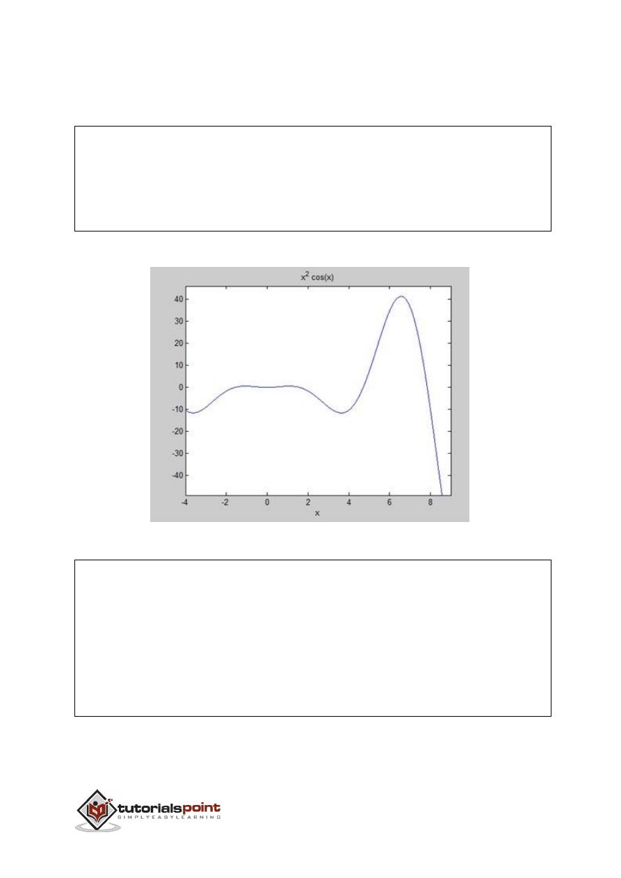
214
Find the area under the curve: f(x) = x
2
cos(x) for −4 ≤ x ≤ 9.
Create a script file and write the following code:
f = x^2*cos(x);
ezplot(f, [-4,9])
a = int(f, -4, 9)
disp('Area: '), disp(double(a));
When you run the file, MATLAB plots the graph:
The output is given below:
a =
8*cos(4) + 18*cos(9) + 14*sin(4) + 79*sin(9)
Area:
0.3326
Following is the Octave equivalent of the above calculation:

215
pkg load symbolic
symbols
x = sym("x");
f = inline("x^2*cos(x)");
ezplot(f, [-4,9])
print -deps graph.eps
[a, ierror, nfneval] = quad(f, -4, 9);
display('Area: '), disp(double(a));

216
MATLAB represents polynomials as row vectors containing coefficients ordered by
descending powers. For example, the equation P(x) = x
4
+ 7x
3
- 5x + 9 could be
represented as:
p = [1 7 0 -5 9];
Evaluating Polynomials
The
polyval
function is used for evaluating a polynomial at a specified value. For
example, to evaluate our previous polynomial
p, at x = 4, type:
p = [1 7 0 -5 9];
polyval(p,4)
MATLAB executes the above statements and returns the following result:
ans =
693
MATLAB also provides the
polyvalm
function for evaluating a matrix polynomial.
A matrix polynomial is a
polynomial
with matrices as variables.
For example, let us create a square matrix X and evaluate the polynomial p, at X:
p = [1 7 0 -5 9];
X = [1 2 -3 4; 2 -5 6 3; 3 1 0 2; 5 -7 3 8];
polyvalm(p, X)
MATLAB executes the above statements and returns the following result:
ans =
2307 -1769 -939 4499
2314 -2376 -249 4695
2256 -1892 -549 4310
26.
POLYNOMIALS

217
4570 -4532 -1062 9269
Finding the Roots of Polynomials
The
roots
function calculates the roots of a polynomial. For example, to calculate
the roots of our polynomial p, type:
p = [1 7 0 -5 9];
r = roots(p)
MATLAB executes the above statements and returns the following result:
r =
-6.8661 + 0.0000i
-1.4247 + 0.0000i
0.6454 + 0.7095i
0.6454 - 0.7095i
The function
poly
is an inverse of the roots function and returns to the polynomial
coefficients. For example:
p2 = poly(r)
MATLAB executes the above statements and returns the following result:
p2 =
1.0000 7.0000 0.0000 -5.0000 9.0000
Polynomial Curve Fitting
The
polyfit
function finds the coefficients of a polynomial that fits a set of data in
a least-squares sense. If x and y are two vectors containing the x and y data to
be fitted to a n-degree polynomial, then we get the polynomial fitting the data by
writing:
p = polyfit(x,y,n)
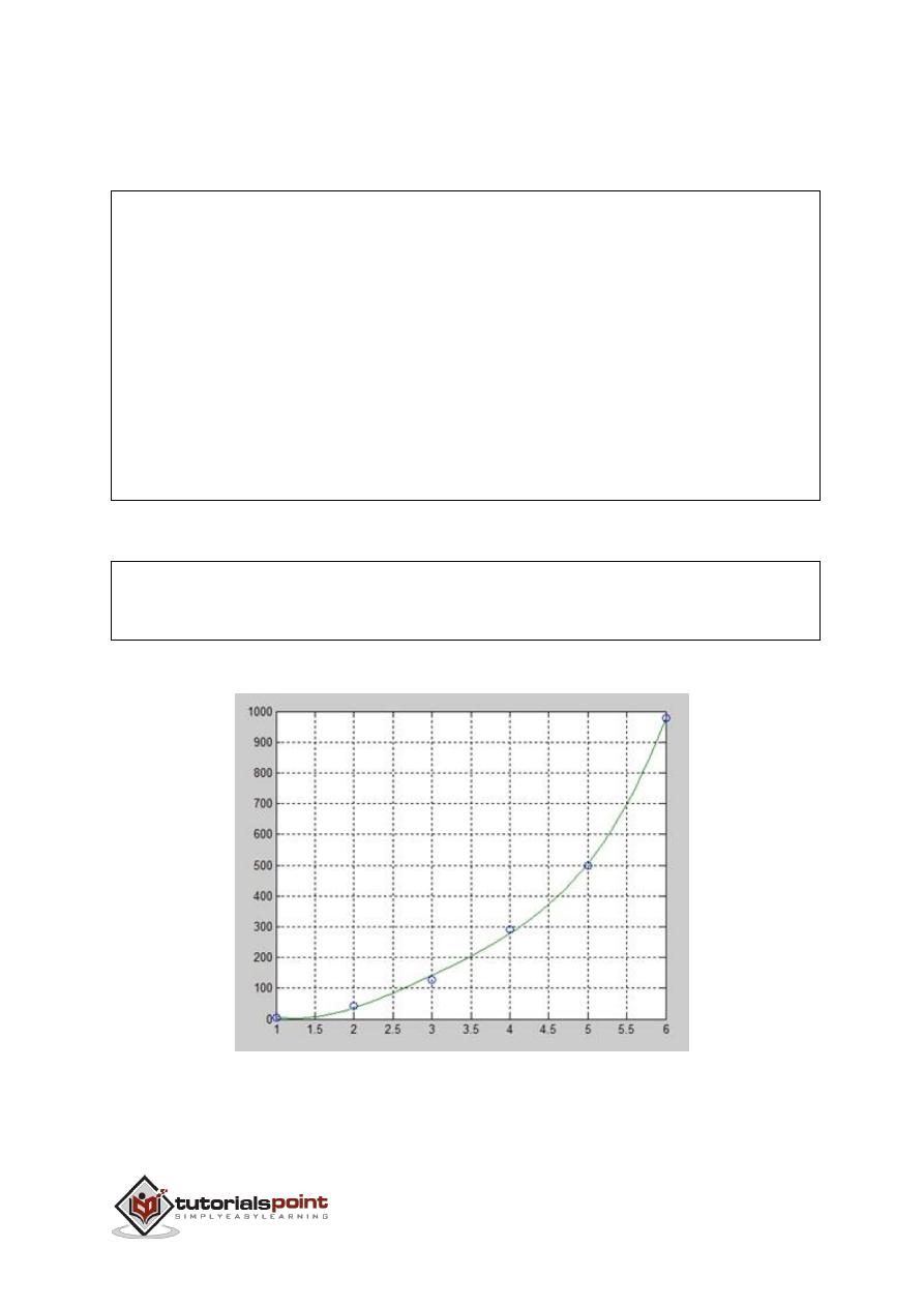
218
Example
Create a script file and type the following code:
x = [1 2 3 4 5 6]; y = [5.5 43.1 128 290.7 498.4 978.67]; %data
p = polyfit(x,y,4) %get the polynomial
% Compute the values of the polyfit estimate over a finer range,
% and plot the estimate over the real data values for comparison:
x2 = 1:.1:6;
y2 = polyval(p,x2);
plot(x,y,'o',x2,y2)
grid on
When you run the file, MATLAB displays the following result:
p =
4.1056 -47.9607 222.2598 -362.7453 191.1250
The following graph will be plotted:
219
MATLAB provides command for working with transforms, such as the Laplace and
Fourier transforms. Transforms are used in science and engineering as a tool for
simplifying analysis and look at data from another angle.
For example, the Fourier transform allows us to convert a signal represented as a
function of time to a function of frequency. Laplace transform allows us to convert
a differential equation to an algebraic equation.
MATLAB provides the
laplace,
fourier
and
fft
commands to work with Laplace,
Fourier and Fast Fourier transforms.
The Laplace Transform
The Laplace transform of a function of time f(t) is given by the following integral:
Laplace transform is also denoted as transform of f(t) to F(s). You can see this
transform or integration process converts f(t), a function of the symbolic variable
t, into another function F(s), with another variable s.
Laplace transform turns differential equations into algebraic ones. To compute a
Laplace transform of a function f(t), write:
laplace(f(t))
Example
In this example, we will compute the Laplace transform of some commonly used
functions.
Create a script file and type the following code:
syms s t a b w
laplace(a)
laplace(t^2)
laplace(t^9)
laplace(exp(-b*t))
27.
TRANSFORMS

220
laplace(sin(w*t))
laplace(cos(w*t))
When you run the file, it displays the following result:
ans =
1/s^2
ans =
2/s^3
ans =
362880/s^10
ans =
1/(b + s)
ans =
w/(s^2 + w^2)
ans =
s/(s^2 + w^2)
The Inverse Laplace Transform
MATLAB allows us to compute the inverse Laplace transform using the
command
ilaplace.
For example,

221
ilaplace(1/s^3)
MATLAB will execute the above statement and display the result:
ans =
t^2/2
Example
Create a script file and type the following code:
syms s t a b w
ilaplace(1/s^7)
ilaplace(2/(w+s))
ilaplace(s/(s^2+4))
ilaplace(exp(-b*t))
ilaplace(w/(s^2 + w^2))
ilaplace(s/(s^2 + w^2))
When you run the file, it displays the following result:
ans =
t^6/720
ans =
2*exp(-t*w)
ans =
cos(2*t)
ans =
ilaplace(exp(-b*t), t, x)

222
ans =
sin(t*w)
ans =
cos(t*w)
The Fourier Transforms
Fourier transforms commonly transforms a mathematical function of time, f(t),
into a new function, sometimes denoted by or F, whose argument is frequency
with units of cycles/s (hertz) or radians per second. The new function is then
known as the Fourier transform and/or the frequency spectrum of the function f.
Example
Create a script file and type the following code in it:
syms x
f = exp(-2*x^2); %our function
ezplot(f,[-2,2]) % plot of our function
FT = fourier(f) % Fourier transform
When you run the file, MATLAB plots the following graph:
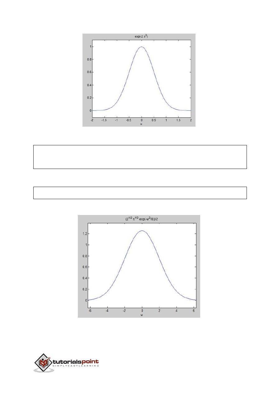
223
The following result is displayed:
FT =
(2^(1/2)*pi^(1/2)*exp(-w^2/8))/2
Plotting the Fourier transform as:
ezplot(FT)
Gives the following graph:
224
Inverse Fourier Transforms
MATLAB provides the
ifourier
command for computing the inverse Fourier
transform of a function. For example,
f = ifourier(-2*exp(-abs(w)))
MATLAB will execute the above statement and display the result:
f =
-2/(pi*(x^2 + 1))

225
GNU Octave is a high-level programming language like MATLAB and it is mostly
compatible with MATLAB. It is also used for numerical computations.
Octave has the following common features with MATLAB:
Matrices are fundamental data type.
It has built-in support for complex numbers.
It has built-in math functions and libraries.
It supports user-defined functions.
GNU Octave is also freely redistributable software. You may redistribute it and/or
modify it under the terms of the GNU General Public License (GPL) as published
by the Free Software Foundation.
MATLAB vs Octave
Most MATLAB programs run in Octave, but some of the Octave programs may not
run in MATLAB because, Octave allows some syntax that MATLAB does not.
For example, MATLAB supports single quotes only, but Octave supports both single
and double quotes for defining strings. If you are looking for a tutorial on Octave,
then kindly go through this tutorial from beginning which covers both MATLAB as
well as Octave.
Compatible Examples
Almost all the examples covered in this tutorial are compatible with MATLAB as
well as Octave. Let's try following example in MATLAB and Octave which produces
same result without any syntax changes:
This example creates a 3D surface map for the function g = xe
-(x2 + y2)
. Create a
script file and type the following code:
[x,y] = meshgrid(-2:.2:2);
g = x .* exp(-x.^2 - y.^2);
surf(x, y, g)
print -deps graph.eps
28.
GNU OCTAVE TUTORIAL

226
When you run the file, MATLAB displays the following 3-D map:
Non-compatible Examples
Though all the core functionality of MATLAB is available in Octave, there are some
functionality for example, Differential & Integration Calculus, which does not
match exactly in both the languages. This tutorial has tried to give both type of
examples where they differed in their syntax.
Consider following example where MATLAB and Octave make use of different
functions to get the area of a curve: f(x) = x
2
cos(x) for −4 ≤ x ≤ 9. Following is
MATLAB version of the code:
f = x^2*cos(x);
ezplot(f, [-4,9])
a = int(f, -4, 9)
disp('Area: '), disp(double(a));
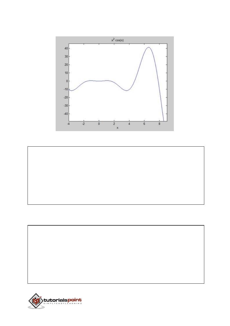
227
When you run the file, MATLAB plots the graph:
The following result is displayed
:
a =
8*cos(4) + 18*cos(9) + 14*sin(4) + 79*sin(9)
Area:
0.3326
But to give area of the same curve in Octave, you will have to make use
of
symbolic package as follows:
pkg load symbolic
symbols
x = sym("x");
f = inline("x^2*cos(x)");

228
ezplot(f, [-4,9])
print -deps graph.eps
[a, ierror, nfneval] = quad(f, -4, 9);
display('Area: '), disp(double(a));

229
Simulink is a simulation and model-based design environment for dynamic and
embedded systems, integrated with MATLAB. Simulink, also developed by
MathWorks, is a data flow graphical programming language tool for modeling,
simulating and analyzing multi-domain dynamic systems. It is basically a graphical
block diagramming tool with customizable set of block libraries.
It allows you to incorporate MATLAB algorithms into models as well as export the
simulation results into MATLAB for further analysis.
Simulink supports:
system-level design
simulation
automatic code generation
testing and verification of embedded systems
There are several other add-on products provided by MathWorks and third-party
hardware and software products that are available for use with Simulink.
The following list gives a brief description of some of them:
Stateflow
allows developing state machines and flow charts.
Simulink Coder
allows the generation of C source code for real-time
implementation of systems automatically.
xPC Target
together with
x86-based real-time systems
provide an
environment to simulate and test Simulink and Stateflow models in real-
time on the physical system.
Embedded Coder
supports specific embedded targets.
HDL Coder
allows to automatically generate synthesizable VHDL and
Verilog.
SimEvents
provides a library of graphical building blocks for modelling
queuing systems.
Simulink is capable of systematic verification and validation of models through
modelling style checking, requirements traceability and model coverage analysis.
Simulink Design Verifier allows you to identify design errors and to generate test
case scenarios for model checking.
29.
SIMULINK
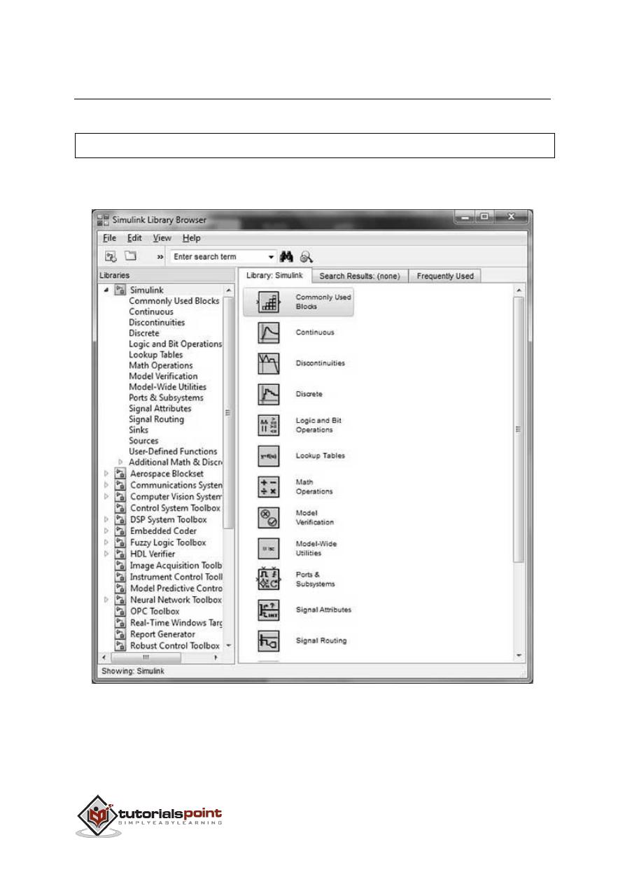
230
Using Simulink
To open Simulink, type in the MATLAB work space:
simulink
Simulink opens with the
Library Browser. The Library Browser is used for
building simulation models.
On the left side window pane, you will find several libraries categorized on the
basis of various systems, clicking on each one will display the design blocks on
the right window pane.
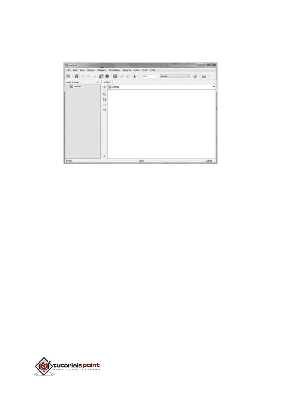
231
Building Models
To create a new model, click the
New
button on the Library Browser's toolbar.
This opens a new untitled model window
A Simulink model is a block diagram.
Model elements are added by selecting the appropriate elements from the Library
Browser and dragging them into the Model window.
Alternately, you can copy the model elements and paste them into the model
window.
Examples
Drag and drop items from the Simulink library to make your project.
For the purpose of this example, two blocks will be used for the simulation -
A
Source
(a signal) and a
Sink
(a scope). A signal generator (the source)
generates an analog signal, which will then be graphically visualized by the
scope(the sink).
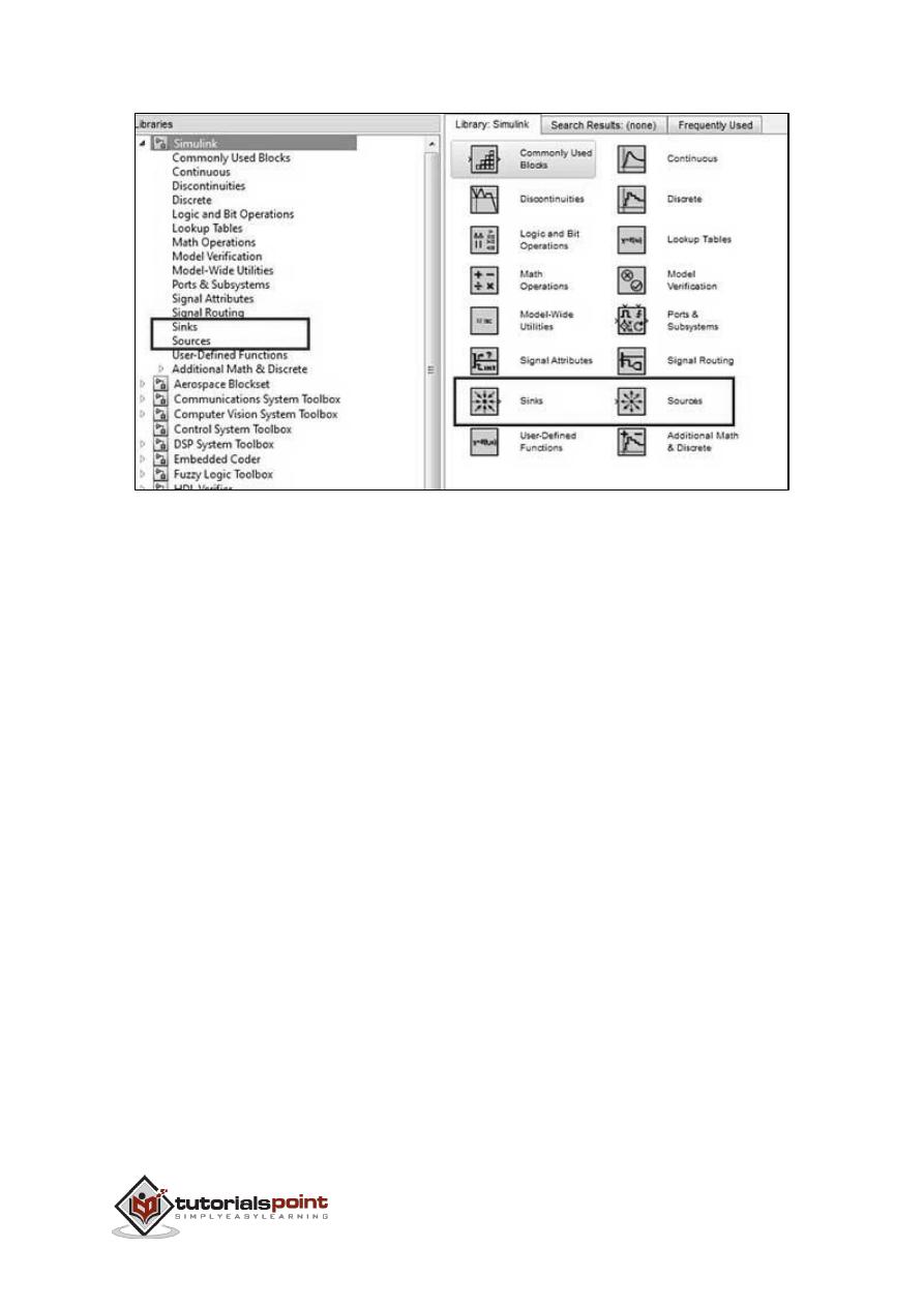
232
Begin by dragging the required blocks from the library to the project window.
Then, connect the blocks together which can be done by dragging connectors from
connection points on one block to those of another.
Let us drag a 'Sine Wave' block into the model.
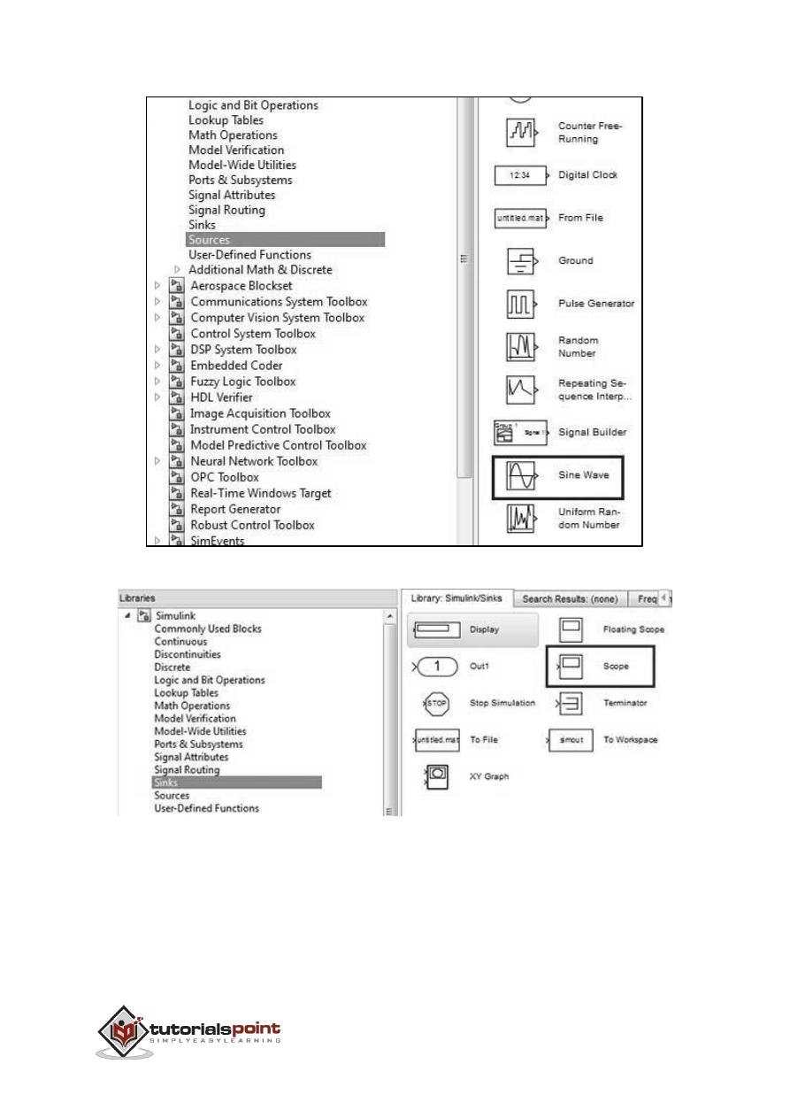
233
Select 'Sinks' from the library and drag a 'Scope' block into the model.
Drag a signal line from the output of the Sine Wave block to the input of the Scope
block.
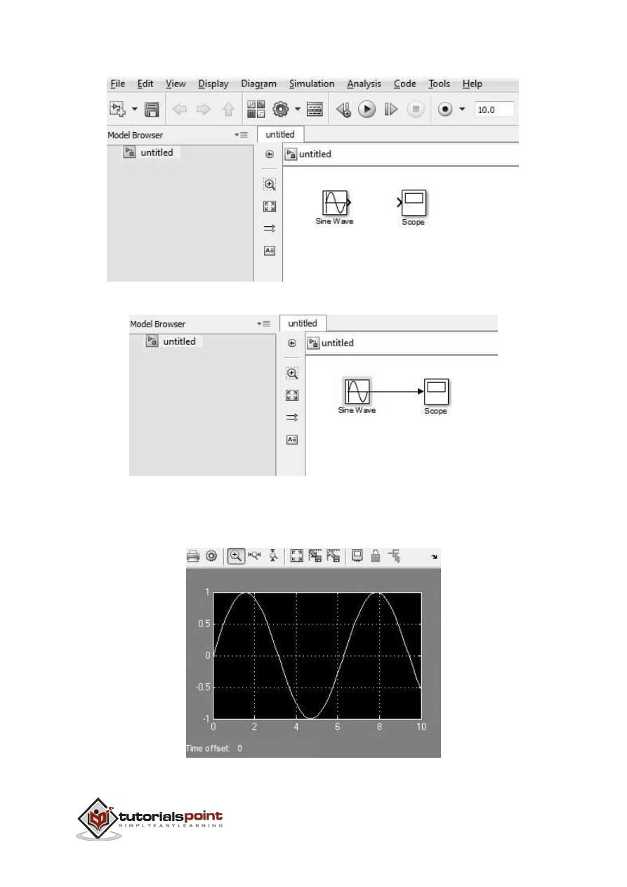
234
Run the simulation by pressing the 'Run' button, keeping all parameters default
(you can change them from the Simulation menu)
You should get the below graph from the scope.