CalcII_ParametricEqns_PolarCoords_Solutions pdf - عبدالرحمن سهيل

CALCULUS II

Solutions to Practice Problems

Parametric Equations and Polar Coordinates

Paul Dawkins

Calculus II

http://tutorial.math.lamar.edu/terms.aspx

Table of Contents

Preface ............................................................................................................................................ 1

Parametric Equations and Polar Coordinates ............................................................................ 1

Introduction ................................................................................................................................................ 1

Parametric Equations and Curves .............................................................................................................. 2

Tangents with Parametric Equations .........................................................................................................47

Area with Parametric Equations ................................................................................................................53

Arc Length with Parametric Equations .....................................................................................................54

Surface Area with Parametric Equations...................................................................................................60

Polar Coordinates ......................................................................................................................................65

Tangents with Polar Coordinates ..............................................................................................................76

Area with Polar Coordinates .....................................................................................................................79

Arc Length with Polar Coordinates ...........................................................................................................88

Surface Area with Polar Coordinates ........................................................................................................90

Arc Length and Surface Area Revisited ....................................................................................................92

Preface

Here are the solutions to the practice problems for my Calculus II notes. Some solutions will
have more or less detail than other solutions. As the difficulty level of the problems increases
less detail will go into the basics of the solution under the assumption that if you’ve reached the
level of working the harder problems then you will probably already understand the basics fairly
well and won’t need all the explanation.

This document was written with presentation on the web in mind. On the web most solutions are
broken down into steps and many of the steps have hints. Each hint on the web is given as a
popup however in this document they are listed prior to each step. Also, on the web each step can
be viewed individually by clicking on links while in this document they are all showing. Also,
there are liable to be some formatting parts in this document intended for help in generating the
web pages that haven’t been removed here. These issues may make the solutions a little difficult
to follow at times, but they should still be readable.

Parametric Equations and Polar Coordinates

Introduction

Here are a set of problems for which no solutions are available. The main intent of these
problems is to have a set of problems available for any instructors who are looking for some extra
problems.

Calculus II

http://tutorial.math.lamar.edu/terms.aspx

Note that some sections will have more problems than others and some will have more or less of
a variety of problems. Most sections should have a range of difficulty levels in the problems
although this will vary from section to section.

Here is a list of topics in this chapter that have problems written for them.

Parametric Equations and Curves

– No problems written yet.

Tangents with Parametric Equations

– No problems written yet.

Area with Parametric Equations

– No problems written yet.

Arc Length with Parametric Equations

– No problems written yet.

Surface Area with Parametric Equations

– No problems written yet.

Polar Coordinates

– No problems written yet.

Tangents with Polar Coordinates

– No problems written yet.

Area with Polar Coordinates

– No problems written yet.

Arc Length with Polar Coordinates

– No problems written yet.

Surface Area with Polar Coordinates

– No problems written yet.

Arc Length and Surface Area Revisited

– No problems written yet.

Parametric Equations and Curves

1. Eliminate the parameter for the following set of parametric equations, sketch the graph of the
parametric curve and give any limits that might exist on x and y.

4 2

3 6

= −

= + −

Step 1
First we’ll eliminate the parameter from this set of parametric equations. For this particular set of
parametric equations we can do that by solving the x equation for t and plugging that into the y equation.

Doing that gives (we’ll leave it to you to verify all the algebra bits…),

(

)

(

)

(

)

3 6

−

→

= +

−

= − +

−

















Step 2
Okay, from this it looks like we have a parabola that opens downward. To sketch the graph of this we’ll
need the x-intercepts, y-intercept and most importantly the vertex.

For notational purposes let’s define

( )

f x

= − +

−

The x-intercepts are then found by solving

( )

f x

. Doing this gives,

Calculus II

http://tutorial.math.lamar.edu/terms.aspx

( )

( )( )

( )

0.2087, 4.7913

− ±

− −

−

− +

− =

→

−

The y-intercept is :

( )

(

)

(

)

0, 1

−

Finally, the vertex is,

( )

5 21

2 4









−





 





−









 







 



−





 







 



Step 3
Before we sketch the graph of the parametric curve recall that all parametric curves have a direction of
motion, i.e. the direction indicating increasing values of the parameter, t in this case.

There are several ways to get the direction of motion for the curve. One is to plug in values of t into the
parametric equations to get some points that we can use to identify the direction of motion.

Here is a table of values for this set of parametric equations.

-1

-7

3
4

5
2

-1

-2

-15

Note that

3
4

is the value of t that give the vertex of the parabola and is not an obvious value of t to use!

In fact, this is a good example of why just using values of t to sketch the graph is such a bad way of
getting the sketch of a parametric curve. It is often very difficult to determine a good set of t’s to use.

For this table we first found the vertex t by using the fact that we actually knew the coordinates of the
vertex (the x-coordinate for this example was the important one) as follows,

4 2

= −

→

Once this value of t was found we chose several values of t to either side for a good representation of t for
our sketch.

Note that, for this case, we used the x-coordinates to find the value of the t that corresponds to the vertex
because this equation was a linear equation and there would be only one solution for t. Had we used the
y-coordinate we would have had to solve a quadratic (not hard to do of course) that would have resulted
in two t’s. The problem is that only one t gives the vertex for this problem and so we’d need to then
check them in the x equation to determine the correct one. So, in this case we might as well just go with
the x equation from the start.

Calculus II

http://tutorial.math.lamar.edu/terms.aspx

Also note that there is an easier way (probably – it will depend on you of course) to determine direction of
motion. Take a quick look at the x equation.

4 2

= −

Because of the minus sign in front of the t we can see that as t increases x must decrease (we can verify
with a quick derivative/Calculus I analysis if we want to).  This means that the graph must be tracing out
from right to left as the table of values above in the table also indicates.

Using a quick Calculus analysis of one, or both, of the parametric equations is often a better and easier
method for determining the direction of motion for a parametric curve. For “simple” parametric
equations we can often get the direction based on a quick glance at the parametric equations and it avoids
having to pick “nice” values of t for a table.

Step 4
We could sketch the graph at this point, but let’s first get any limits on x and y that might exist.

Because we have a parabola that opens downward and we’ve not restricted t’s in any way we know that
we’ll get the whole parabola.  This in turn means that we won’t have any limits at all on x but y must
satisfy

≤

(remember the y-coordinate of the vertex?).

So, formally here are the limits on x and y.

−∞ < < ∞

≤

Note that having the limits on x and y will often help with the actual graphing step so it’s often best to get
them prior to sketching the graph. In this case they don’t really help as we can sketch the graph of a
parabola without these limits, but it’s just good habit to be in so we did them first anyway.

Step 5
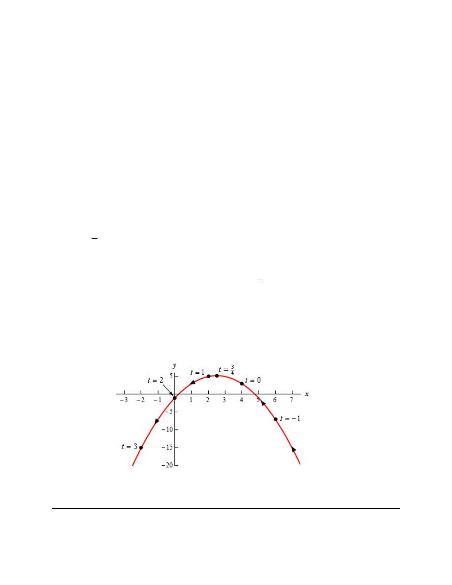
Finally, here is a sketch of the parametric curve for this set of parametric equations.

For this sketch we included the points from our table because we had them but we won’t always include
them as we are often only interested in the sketch itself and the direction of motion.

Calculus II

http://tutorial.math.lamar.edu/terms.aspx

2. Eliminate the parameter for the following set of parametric equations, sketch the graph of the
parametric curve and give any limits that might exist on x and y.

4 2

3 6

= −

= + −

≤ ≤

Step 1
Before we get started on this problem we should acknowledge that this problems is really just a restriction
on the first problem (i.e. it is the same problem except we restricted the values of t to use). As such we
could just go back to the first problem and modify the sketch to match the restricted values of t to get a
quick solution and in general that is how a problem like this would work.

However, we’re going to approach this solution as if this was its own problem because we won’t always
have the more general problem worked ahead of time. So, let’s proceed with the problem assuming we
haven’t worked the first problem in this section.

First we’ll eliminate the parameter from this set of parametric equations. For this particular set of
parametric equations we can do that by solving the x equation for t and plugging that into the y equation.

Doing that gives (we’ll leave it to you to verify all the algebra bits…),

(

)

(

)

(

)

3 6

−

→

= +

−

= − +

−

















Step 2
Okay, from this it looks like we have a parabola that opens downward. To sketch the graph of this we’ll
need the x-intercepts, y-intercept and most importantly the vertex.

For notational purposes let’s define

( )

f x

= − +

−

The x-intercepts are then found by solving

( )

f x

. Doing this gives,

( )

( )( )

( )

0.2087, 4.7913

− ±

− −

−

− +

− =

→

−

The y-intercept is :

( )

(

)

(

)

0, 1

−

Finally, the vertex is,

( )

5 21

2 4









−





 





−









 







 



−





 







 



Calculus II

http://tutorial.math.lamar.edu/terms.aspx

There are several ways to get the direction of motion for the curve. One is to plug in values of t into the
parametric equations to get some points that we can use to identify the direction of motion.

Here is a table of values for this set of parametric equations. Also note that because we’ve restricted the
value of t for this problem we need to keep that in mind as we chose values of t to use.

3
4

5
2

-1

-2

-15

Note that

3
4

is the value of t that give the vertex of the parabola and is not an obvious value of t to use!

4 2

= −

→

4 2

= −

Because of the minus sign in front of the t we can see that as t increases x must decrease (we can verify
with a quick derivative/Calculus I analysis if we want to). This means that the graph must be tracing out
from right to left as the table of values above in the table also indicates.

Using a quick Calculus analysis of one, or both, of the parametric equations is often a better and easier
method for determining the direction of motion for a parametric curve. For “simple” parametric
equations we can often get the direction based on a quick glance at the parametric equations and it avoids
having to pick “nice” values of t for a table.

Step 4
Let’s now get the limits on x and y and note that we really do need these before we start sketching the
curve!

Calculus II

http://tutorial.math.lamar.edu/terms.aspx

In this case we have a parabola that opens downward and we could use that to get a general set of limits
on x and y. However, for this problem we’ve also restricted the values of t that we’re using and that will
in turn restrict the values of x and y that we can use for the sketch of the graph.

As we discussed above we know that the graph will sketch out from right to left and so the rightmost
value of x will come from

, which is

. Likewise the leftmost value of y will come from

which is

= −

. So, from this we can see the limits on x must be

− ≤ ≤

For the limits on the y we’ve got be a little more careful. First, we know that the vertex occurs in the
given range of t’s and because the parabola opens downward the largest value of y we will have is

i.e. the y-coordinate of the vertex. Also because the parabola opens downward we know that the smallest
value of y will have to be at one of the endpoints. So, for

we have

and for

we have

= −

. Therefore, the limits on y must be

− ≤ ≤

So, putting all this together here are the limits on x and y.

− < <

− ≤ ≤

Note that for this problem we must have these limits prior to the sketching step. Because we’ve restricted
the values of t to use we will have limits on x and y (as we just discussed) and so we will only have a
portion of the graph of the full parabola. Having these limits will allow us to get the sketch of the
parametric curve.

Step 5
Finally, here is a sketch of the parametric curve for this set of parametric equations.

For this sketch we included the points from our table because we had them but we won’t always include
them as we are often only interested in the sketch itself and the direction of motion.

Also note that it is vitally important that we not extend the graph past the

and

points. If we

extend the graph past these points we are implying that the graph will extend past them and of course it
doesn’t!

Calculus II

http://tutorial.math.lamar.edu/terms.aspx

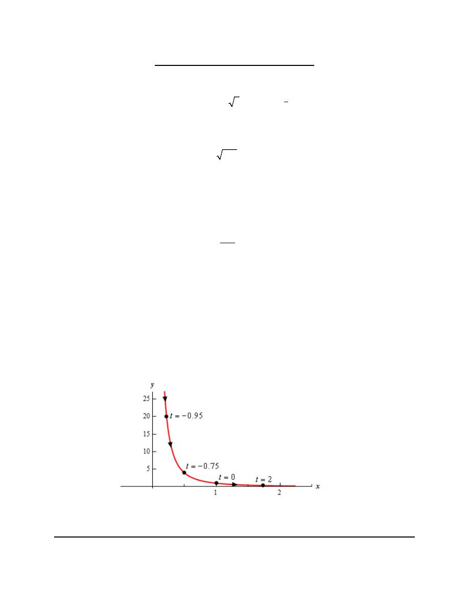
3. Eliminate the parameter for the following set of parametric equations, sketch the graph of the
parametric curve and give any limits that might exist on x and y.

> −

Step 1
First we’ll eliminate the parameter from this set of parametric equations. For this particular set of
parametric equations that is actually really easy to do if we notice the following.

⇒

= +

With this we can quickly convert the y equation to,

Step 2

At this point we can get limits on x and y pretty quickly so let’s do that.

First, we know that square roots always return positive values (or zero of course) and so from the x
equation we see that we must have

. Note as well that this must be a strict inequality because the

inequality restricting the range of t’s is also a strict inequality. In other words, because we aren’t allowing

= −

we will never get

Speaking of which, you do see why we’ve restricted the t’s don’t you?

Now, from our restriction on t we know that

1 0

+ >

and so from the y parametric equation we can see

that we also must have

. This matches what we see from the equation without the parameter we

found in Step 1.

So, putting all this together here are the limits on x and y.

Note that for this problem these limits are important (or at least the x limits are important). Because of
the x limit we get from the parametric equation we can see that we won’t have the full graph of the
equation we found in the first step. All we will have is the portion that corresponds to

Calculus II

http://tutorial.math.lamar.edu/terms.aspx

-0.95

0.2236

-0.75

0.5

1
3

Note that there is an easier way (probably – it will depend on you of course) to determine direction of
motion. Take a quick look at the x equation.

Increasing the value of t will also cause t + 1 to increase and the square root will also increase (we can
verify with a quick derivative/Calculus I analysis if we want to). This means that the graph must be
tracing out from left to right as the table of values above in the table supports.

Likewise, we could use the y equation.

Again, we know that as t increases so does t + 1. Because the t + 1 is in the denominator we can further
see that increasing this will cause the fraction, and hence y, to decrease. This means that the graph must
be tracing out from top to bottom as both the x equation and table of values supports.

Using a quick Calculus analysis of one, or both, of the parametric equations is often a better and easier
method for determining the direction of motion for a parametric curve. For “simple” parametric
equations we can often get the direction based on a quick glance at the parametric equations and it avoids
having to pick “nice” values of t for a table.

Step 4
Finally, here is a sketch of the parametric curve for this set of parametric equations.

For this sketch we included the points from our table because we had them but we won’t always include
them as we are often only interested in the sketch itself and the direction of motion.

Calculus II

http://tutorial.math.lamar.edu/terms.aspx

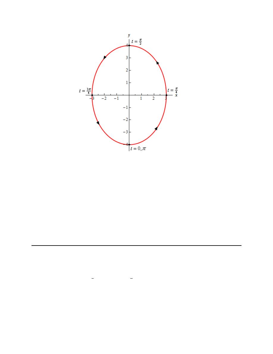
4. Eliminate the parameter for the following set of parametric equations, sketch the graph of the
parametric curve and give any limits that might exist on x and y.

( )

3sin

4 cos

= −

≤ ≤

Step 1
First we’ll eliminate the parameter from this set of parametric equations. For this particular set of
parametric equations we will make use of the well-known trig identity,

( )

cos

sin

We can solve each of the parametric equations for sine and cosine as follows,

( )

sin

cos

= −

Plugging these into the trig identity gives,





 

−

⇒





 





 

Therefore, the parametric curve will be some or all of the ellipse above.

We have to be careful when eliminating the parameter from a set of parametric equations.  The graph of
the resulting equation in only x and y may or may not be the graph of the parametric curve. Often,
although not always, the parametric curve will only be a portion of the curve from the equation in terms
of only x and y. Another situation that can happen is that the parametric curve will retrace some or all of
the curve from the equation in terms of only x and y more than once.

The next few steps will help us to determine just how much of the ellipse we have and if it retraces the
ellipse, or a portion of the ellipse, more than once.

Before we proceed with the rest of the problem let’s fist note that there is really no set order for doing the
steps.  They can often be done in different orders and in some cases may actually be easier to do in
different orders.  The order we’ll be following here is used simply because it is the order that I’m used to
working them in. If you find a different order would be best for you then that is the order you should use.

Step 2

At this point we can get a good idea on what the limits on x and y are going to be so let’s do that.
Note that often we won’t get the actual limits on x and y in this step. All we are really finding
here is the largest possible range of limits for x and y. Having these can sometimes be useful for
later steps and so we’ll get them here.

We can use our knowledge of sine and cosine to get the following inequalities. Note as discussed above
however that these may not be the limits on x and y we are after.

Calculus II

http://tutorial.math.lamar.edu/terms.aspx

( )

1 sin

1 cos

3sin

4 cos

− ≤

≤

− ≤

≤

− ≤

≤

≥ −

− ≤ ≤

Note that to find these limits in general we just start with the appropriate trig function and then build up
the equation for x and y by first multiplying the trig function by any coefficient, if present, and then
adding/subtracting any numbers that might be present (not needed in this case). This, in turn, gives us the
largest possible set of limits for x and y.  Just remember to be careful when multiplying an inequality by a
negative number. Don’t forget to flip the direction of the inequalities when doing this.

Now, at this point we need to be a little careful.  What we’ve actually found here are the largest possible
inequalities for the limits on x and y.  This set of inequalities for the limits on x and y assume that the
parametric curve will be completely traced out at least once for the range of t’s we were given in the
problem statement. It is always possible that the curve will not trace out a full trace in the given range of
t’s.  In a later step we’ll determine if the parametric curve does trace out a full trace and hence determine
the actual limits on x and y.

Before we move onto the next step there are a couple of issues we should quickly discuss.

First, remember that when we talk about the parametric curve tracing out once we are not necessarily
talking about the ellipse itself being fully traced out.  The parametric curve will be at most the full ellipse
and we haven’t determined just yet how much of the ellipse the parametric curve will trace out. So, one
trace of the parametric curve refers to the largest portion of the ellipse that the parametric curve can
possibly trace out given no restrictions on t.

Second, if we can’t completely determine the actual limits on x and y at this point why did we do them
here? In part we did them here because we can and the answer to this step often does end up being the
limits on x and y. Also, there are times where knowing the largest possible limits on x and/or y will be
convenient for some of the later steps.

Finally, we can sometimes get these limits from the sketch of the parametric curve. However, there are
some parametric equations that we can’t easily get the sketch without doing this step. We’ll eventually do
some problems like that.

Step 3
Before we sketch the graph of the parametric curve recall that all parametric curves have a direction of
motion, i.e. the direction indicating increasing values of the parameter, t in this case.

There are several ways to get the direction of motion for the curve. One is to plug in values of t into the
parametric equations to get some points that we can use to identify the direction of motion.

Here is a table of values for this set of parametric equations. In this case we were also given a range of t’s
and we need to restrict the t’s in our table to that range.

-4

Calculus II

http://tutorial.math.lamar.edu/terms.aspx

-3

-4

Now, this table seems to suggest that the parametric equation will follow the ellipse in a counter
clockwise rotation. It also seems to suggest that the ellipse will be traced out exactly once.

However, tables of values for parametric equations involving sine and/or cosine equations can be
deceptive.

Because sine and cosine oscillate it is possible to choose “bad” values of t that suggest a single trace when
in fact the curve is tracing out faster than we realize and it is in fact tracing out more than once. We’ll
need to do some extra analysis to verify if the ellipse traces out once or more than once.

Also, just because the table suggests a particular direction doesn’t actually mean it is going in that
direction. It could be moving in the opposite direction at a speed that just happens to match the points
you got in the table. Go back to the notes and check out Example 5. Plug in the points we used in our
table above and you’ll get a set of points that suggest the curve is tracing out clockwise when in fact it is
tracing out counter clockwise!

Note that because this is such a “bad” way of getting the direction of motion we put it in its own step so
we could discuss it in detail. The actual method we’ll be using is in the next step and we’ll not be doing
table work again unless it is absolutely required for some other part of the problem.

Step 4
As suggested in the previous step the table of values is not a good way to get direction of motion for
parametric curves involving trig function so let’s go through a much better way of determining the
direction of motion.  This method takes a little time to think things through but it will always get the
correct direction if you take the time.

First, let’s think about what happens if we start at

and increase t to

As we cover this range of t’s we know that cosine starts at 1, decreasing through zero and finally stops at -
1. So, that means that y will start at

= −

(i.e. where cosine is 1), go through the x-axis (i.e. where

cosine is zero) and finally stop at

(i.e. where cosine is -1). Now, this doesn’t give us a direction of

motion as all it really tells us that y increases and it could do this following the right side of the ellipse
(i.e. counter clockwise) or it could do this following the left side of the ellipse (i.e. clockwise).

So, let’s see what the behavior of sine in this range tells us. Starting at

we know that sine will be

zero and so x will also be zero. As t increases to

we know that sine increases from zero to one and

so x will increase from zero to three. Finally, as we further increase t to

sine will decrease from

one back to zero and so x will also decrease from three to zero.

So, taking the x and y analysis above together we can see that at

the curve will start at the point

(

)

0, 4

−

. As we increase t to

the curve will have to follow the ellipse with increasing x and y until

it hits the point

( )

3, 0

. The only way we can reach this second point and have the correct increasing

behavior for both x and y is to move in a counter clockwise direction along the right half of the ellipse.

Calculus II

http://tutorial.math.lamar.edu/terms.aspx

If we further increase t from

we can see that y must continue to increase but x now

decreases until we get to the point

( )

0, 4

and again the only way we can reach this third point and have

the required increasing/decreasing information for y/x respectively is to be moving in a counter clockwise
direction along the right half.

We can do a similar analysis increasing t from

to see that we must still move in a

counter clockwise direction that takes us through the point

(

)

3, 0

−

and then finally ending at the point

(

)

0, 4

−

So, from this analysis we can see that the curve must be tracing out in a counter clockwise direction.

This analysis seems complicated and maybe not so easy to do the first few times you see it. However,
once you do it a couple of times you’ll see that it’s not quite as bad as it initially seems to be. Also, it
really is the only way to guarantee that you’ve got the correct direction of motion for the curve when
dealing with parametric equations involving sine and/or cosine.

If you had trouble visualizing how sine and cosine changed as we increased t you might want to do a
quick sketch of the graphs of sine and cosine and you’ll see right away that we were correct in our
analysis of their behavior as we increased t.

Step 5
Okay, in the last step notice that we also showed that the curve will trace the ellipse out exactly once in
the given range of t’s. However, let’s assume that we hadn’t done the direction analysis yet and see if we
can determine this without the direction analysis.

This is actually pretty simple to do, or at least simpler than the direction analysis. All it requires is that
you know where sine and cosine are zero, 1 and -1. If you recall your unit circle it’s always easy to know
where sine and cosine have these values. We’ll also be able to verify the ranges of x and y found in Step
2 were in fact the actual ranges for x and y.

Let’s start with the “initial” point on the curve, i.e. the point at the left end of our range of t’s,

this case. Where you start this analysis is really dependent upon the set of parametric equations, the
parametric curve and/or if there is a range of t’s given. Good starting points are the “initial” point, one of
the end points of the curve itself (if the curve does have endpoints) or

. Sometimes one option will

be better than the others and other times it won’t matter.

In this case two of the options are the same point so it seems like a good point to use.

So, at

we are at the point

(

)

0, 4

−

. We know that the parametric curve is some or all of the ellipse

we found in the first step. So, at this point let’s assume it is the full ellipse and ask ourselves the
following question. When do we get back to this point? Or, in other words, what is the next value of t

after

(since that is the point we choose to start off with) are we back at the point

(

)

0, 4

−

Before doing this let’s quickly note that if the parametric curve doesn’t get back to this point we’ll
determine that in the following analysis and that will be useful in helping us to determine how much of
the ellipse will get traced out by the parametric curve.

Calculus II

http://tutorial.math.lamar.edu/terms.aspx

Okay let’s back to the analysis. In order to be at the point

(

)

0, 4

−

we know we must have

( )

sin

(only way to get

!) and we must have

( )

cos

(only way to get

= −

!). For

we know

that

( )

sin

, 2 , 3 ,

π π π



and likewise we know that

( )

cos

2 , 4 , 6 ,

π π π



. The

first value of t that is in both lists is

and so this is the next value of t that will put us at that point.

This tells us several things. First, we found that the parametric equation will get back to the initial point
and so it is possible for the parametric equation to trace out the full ellipse.

Secondly, we got back to the point

(

)

0, 4

−

at the very last t from the range of t’s we were given in the

problem statement and so the parametric curve will trace out the ellipse exactly once for the given range
of t’s.

Finally, from this analysis we found the parametric curve traced out the full ellipse in the range of t’s
given in the problem statement and so we know now that the limits of x and y we found in Step 2 are in
fact the actual limits on x and y for this curve.

As a final comment from this step let’s note that this analysis in this step was a little easier than normal
because the argument of the trig functions was just a t as opposed to say 2t or

1
3

which does make the

analysis a tiny bit more complicated. We’ll see how to deal with these kinds of arguments in the next
couple of problems.

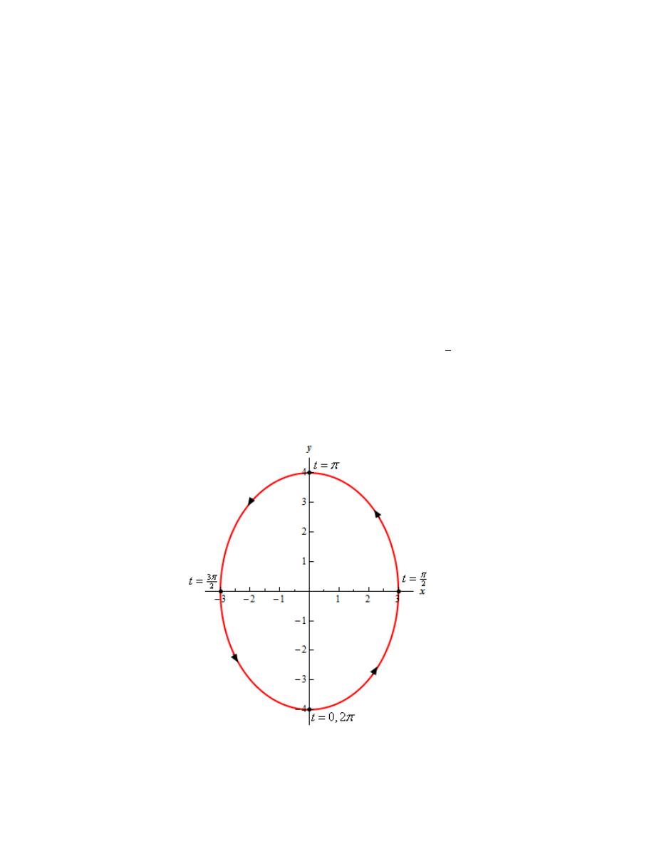
Step 6
Finally, here is a sketch of the parametric curve for this set of parametric equations.

Calculus II

http://tutorial.math.lamar.edu/terms.aspx

For this sketch we included the points from our table because we had them but we won’t always include
them as we are often only interested in the sketch itself and the direction of motion.

Also, because the problem asked for it here are the formal limits on x and y for this parametric curve.

− ≤ ≤

As a final set of thoughts for this problem you really should go back and make sure you understand the
processes we went through in Step 4 and Step 5. Those are often the best way of getting at the
information we found in those steps. The processes can seem a little mysterious at first but once you’ve
done a couple you’ll find it isn’t as bad as they might have first appeared.

Also, for the rest of the problems in this section we’ll build a table of t values only if it is absolutely
necessary for the problem. In other words, the process we used in Step 4 and 5 will be the processes we’ll
be using to get direction of motion for the parametric curve and to determine if the curve is traced out
more than once or not.

You should also take a look at problems 5 and 6 in this section and contrast the number of traces of the
curve with this problem. The only difference in the set of parametric equations in problems 4, 5 and 6 is
the argument of the trig functions. After going through these three problems can you reach any
conclusions on how the argument of the trig functions will affect the parametric curves for this type of
parametric equations?

5. Eliminate the parameter for the following set of parametric equations, sketch the graph of the
parametric curve and give any limits that might exist on x and y.

( )

3sin 2

4 cos 2

= −

≤ ≤

Step 1
First we’ll eliminate the parameter from this set of parametric equations. For this particular set of
parametric equations we will make use of the well-known trig identity,

( )

cos

sin

We can solve each of the parametric equations for sine and cosine as follows,

( )

sin 2

cos 2

= −

Plugging these into the trig identity (remember the identity holds as long as the argument of both trig
functions, 2t in this case, is the same) gives,





 

−

⇒





 





 

Therefore, the parametric curve will be some or all of the ellipse above.

Calculus II

http://tutorial.math.lamar.edu/terms.aspx

We have to be careful when eliminating the parameter from a set of parametric equations.  The graph of
the resulting equation in only x and y may or may not be the graph of the parametric curve. Often,
although not always, the parametric curve will only be a portion of the curve from the equation in terms
of only x and y. Another situation that can happen is that the parametric curve will retrace some or all of
the curve from the equation in terms of only x and y more than once.

This observation is especially important for this problem. The next few steps will help us to determine
just how much of the ellipse we have and if it retraces the ellipse, or a portion of the ellipse, more than
once.

Before we proceed with the rest of the problem let’s fist note that there is really no set order for doing the
steps.  They can often be done in different orders and in some cases may actually be easier to do in
different orders.  The order we’ll be following here is used simply because it is the order that I’m used to
working them in. If you find a different order would be best for you then that is the order you should use.

Step 2

We can use our knowledge of sine and cosine to determine the limits on x and y as follows,

( )

1 sin 2

1 cos 2

3sin 2

4 cos 2

− ≤

≤

− ≤

≤

− ≤

≤

≥ −

− ≤ ≤

Calculus II

http://tutorial.math.lamar.edu/terms.aspx

Second, if we can’t completely determine the actual limits on x and y at this point why did we do them
here? In part we did them here because we can and the answer to this step often does end up being the
limits on x and y. Also, there are times where knowing the largest possible limits on x and/or y will be
convenient for some of the later steps.

Finally, we can sometimes get these limits from the sketch of the parametric curve. However, there are
some parametric equations that we can’t easily get the sketch without doing this step. We’ll eventually do
some problems like that.

Step 3
Before we sketch the graph of the parametric curve recall that all parametric curves have a direction of
motion, i.e. the direction indicating increasing values of the parameter, t in this case.

In previous problems one method we looked at was to build a table of values for a sampling of t’s in the
range provided. However, as we discussed in Problem 4 of this section tables of values for parametric
equations involving trig functions they can be deceptive and so we aren’t going to use them to determine
the direction of motion for this problem.

Also, as noted in the discussion in Problem 4 it also might help to have the graph of sine and cosine
handy to look at since we’ll be talking a lot about the behavior of sine/cosine as we increase the argument.

So for this problem we’ll just do the analysis of the behavior of sine and cosine in the range of t’s we
were provided to determine the direction of motion. We’ll be doing a quicker version of the analysis here
than we did in Problem 4 so you might want to go back and check that problem out if you have trouble
following everything we’re going here.

Let’s start at

since that is the first value of t in the range of t’s we were given in the problem. This

means we’ll be starting the parametric curve at the point

(

)

0, 4

−

Now, what happens if we start to increase t? First, if we increase t then we also increase 2t, the argument

of the trig functions in the parametric equations. So, what does this mean for

( )

sin 2t

and

( )

cos 2t

Well initially, we know that

( )

sin 2t

will increase from zero to one and at the same time

( )

cos 2t

will

also have to decrease from one to zero.

So, this means that x (given by

( )

3sin 2

) will have to increase from 0 to 3. Likewise, it means that

y (given by

( )

4 cos 2

= −

) will have to increase from -4 to 0. For the y equation note that while the

cosine is decreasing the minus sign on the coefficient means that y itself will actually be increasing.

Because this behavior for x and y must be happening at simultaneously we can see that the only

possibility is for the parametric curve to start at

(

)

0, 4

−

and as we increase the value of t we must move to

the right in the counter clockwise direction until we reach the point

( )

3, 0

Okay, we’re now at the point

( )

3, 0

, so

( )

sin 2

and

( )

cos 2

. Let’s continue to increase t. A

further increase of t will force

( )

sin 2t

to decrease from 1 to 0 and at the same time

( )

cos 2t

will

decrease from 0 to -1.

Calculus II

http://tutorial.math.lamar.edu/terms.aspx

In terms of x and y this means that, at the same time, x will now decrease from 3 to 0 while y will continue
to increase from 0 to 4 (again the minus sign on the y equation means y must increase as the cosine
decreases from 0 to -1). So, we must be continuing to move in a counter clockwise direction until we

reach the point

( )

0, 4

For the remainder we’ll go a little quicker in the analysis and just discuss the behavior of x and y and skip
the discussion of the behavior of the sine and cosine.

Another increase in t will force x to decrease from 0 to -3 and at the same time y will have to also
decrease from 4 to 0. The only way for this to happen simultaneously is to move along the ellipse starting

that

( )

0, 4

in a counter clockwise motion until we reach

(

)

3, 0

−

Continuing to increase t and we can see that, at the same time, x will increase from -3 to 0 and y will
decrease from 0 to -4. Or, in other words we’re moving along the ellipse in a counter clockwise motion

from

(

)

3, 0

−

(

)

0, 4

−

At this point we’ve gotten back to the starting point and we got back to that point by always going in a
counter clockwise direction and did not retrace any portion of the graph and so we can now safely say that
the direction of motion for this curve will always counter clockwise.

We have to be very careful here to continue the analysis until we get back to the starting point and see just
how we got back there. It is possible, as we’ll see in later problems, for us to get back there by retracing
back over the curve. This will have an effect on the direction of motion for the curve (i.e. the direction
will change!). In this case however since we got back to the starting point without retracing any portion
of the curve we know the direction will remain counter clockwise.

Step 4
Let’s now think about how much of the ellipse is actually traced out or if the ellipse is traced out more
than once for the range of t’s we were given in the problem. We’ll also be able to verify if the ranges of x
and y we found in Step 2 are the correct ones or if we need to modify them (and we’ll also determine just
how to modify them if we need to).

Be careful to not draw any conclusions about how much of the ellipse is traced out from the analysis in
the previous step. If we follow that analysis we see a full single trace of the ellipse. However, we didn’t
ever really mention any values of t with the exception of the starting value. Because of that we can’t
really use the analysis in the previous step to determine anything about how much of the ellipse we trace
out or how many times we trace the ellipse out.

Let’s go ahead and start this portion out at the same value of t we started with in the previous step. So, at

we are at the point

(

)

0, 4

−

. Now, when do we get back to this point? Or, in other words, what is

the next value of t after

(since that is the point we choose to start off with) are we at the point

(

)

0, 4

−

Calculus II

http://tutorial.math.lamar.edu/terms.aspx

In order to be at this point we know we must have

( )

sin 2

(only way to get

!) and we must

have

( )

cos 2

(only way to get

= −

!). Note the arguments of the sine and cosine! That is very

important for this step.

Now, for

we know that

( )

sin 2

, 2 , 3 ,

π π π



and likewise we know that

( )

cos 2

2 , 4 , 6 ,

π π π



. Again, note the arguments of sine and cosine here! Because we want

( )

sin 2t

and

( )

cos 2t

to have certain values we need to determine the values of 2t we need to achieve the values

of sine and cosine that we are looking for.

The first value of 2t that is in both lists is

. This now tells us the value of t we need to get back

to the starting point. We just need to solve this for t!

⇒

So, we will get back to the starting point, without retracing any portion of the ellipse, important in some
later problems, when we reach

But this is in the middle of the range of t’s we were given! So, just what does this mean for us? Well

first of all, provided the argument of the sine/cosine is only in terms of t, as opposed to

for

example, the “net” range of t’s for one trace will always be the same. So, we got one trace in the range of

≤ ≤

and so the “net” range of t’s here is

− =

and so any range of t’s that span

will trace

out the ellipse exactly once.

This means that the ellipse will also trace out exactly once in the range

≤ ≤

. So, in this case, it

looks like the ellipse will be traced out twice in the range

≤ ≤

This analysis also has shown us that the parametric curve traces out the full ellipse in the range of t’s
given in the problem statement (more than once in fact!) and so we know now that the limits of x and y
we found in Step 2 are in fact the actual limits on x and y for this curve.

Before we leave this step we should note that once you get pretty good at the direction analysis we did in
Step 3 you can combine the analysis Steps 3 and 4 into a single step to get both the direction and portion
of the curve that is traced out. Initially however you might find them a little easier to do them separately.

Step 5
Finally, here is a sketch of the parametric curve for this set of parametric equations.

Calculus II

http://tutorial.math.lamar.edu/terms.aspx

For this sketch we included a set of t’s to illustrate a handful of points and their corresponding values of
t’s. For some practice you might want to follow the analysis from Step 4 to see if you can verify the
values of t for the other three points on the graph. It would, of course, be easier to just plug them in to
verify, but the practice of the process of the Step 4 analysis might be useful to you.

Also, because the problem asked for it here are the formal limits on x and y for this parametric curve.

− ≤ ≤

You should also take a look at problems 4 and 6 in this section and contrast the number of traces of the
curve with this problem. The only difference in the set of parametric equations in problems 4, 5 and 6 is
the argument of the trig functions. After going through these three problems can you reach any
conclusions on how the argument of the trig functions will affect the parametric curves for this type of
parametric equations?

6. Eliminate the parameter for the following set of parametric equations, sketch the graph of the
parametric curve and give any limits that might exist on x and y.

( )

3sin

4 cos

= −

≤ ≤

Step 1
First we’ll eliminate the parameter from this set of parametric equations. For this particular set of
parametric equations we will make use of the well-known trig identity,

( )

cos

sin

Calculus II

http://tutorial.math.lamar.edu/terms.aspx

We can solve each of the parametric equations for sine and cosine as follows,

( )

sin

cos

= −

Plugging these into the trig identity (remember the identity holds as long as the argument of both trig
functions,

1
3

in this case, is the same) gives,





 

−

⇒





 





 

Therefore, the parametric curve will be some or all of the ellipse above.

We have to be careful when eliminating the parameter from a set of parametric equations.  The graph of
the resulting equation in only x and y may or may not be the graph of the parametric curve. Often,
although not always, the parametric curve will only be a portion of the curve from the equation in terms
of only x and y. Another situation that can happen is that the parametric curve will retrace some or all of
the curve from the equation in terms of only x and y more than once.

This observation is especially important for this problem. The next few steps will help us to determine
just how much of the ellipse we have and if it retraces the ellipse, or a portion of the ellipse, more than
once.

Before we proceed with the rest of the problem let’s fist note that there is really no set order for doing the
steps.  They can often be done in different orders and in some cases may actually be easier to do in
different orders.  The order we’ll be following here is used simply because it is the order that I’m used to
working them in. If you find a different order would be best for you then that is the order you should use.

Step 2

We can use our knowledge of sine and cosine to determine the limits on x and y as follows,

( )

1 sin

1 cos

3sin

4 cos

− ≤

≤

− ≤

≤

− ≤

≤

≥ −

− ≤ ≤

Calculus II

http://tutorial.math.lamar.edu/terms.aspx

Now, at this point we need to be a little careful.  What we’ve actually found here are the largest possible
inequalities for the limits on x and y.  This set of inequalities for the limits on x and y assume that the
parametric curve will be completely traced out at least once for the range of t’s we were given in the
problem statement. It is always possible that the curve will not trace out a full trace in the given range of
t’s.  In a later step we’ll determine if the parametric curve does trace out a full trace and hence determine
the actual limits on x and y.

Before we move onto the next step there are a couple of issues we should quickly discuss.

First, remember that when we talk about the parametric curve tracing out once we are not necessarily
talking about the ellipse itself being fully traced out.  The parametric curve will be at most the full ellipse
and we haven’t determined just yet how much of the ellipse the parametric curve will trace out. So, one
trace of the parametric curve refers to the largest portion of the ellipse that the parametric curve can
possibly trace out given no restrictions on t.  This is especially important for this problem!

Second, if we can’t completely determine the actual limits on x and y at this point why did we do them
here? In part we did them here because we can and the answer to this step often does end up being the
limits on x and y. Also, there are times where knowing the largest possible limits on x and/or y will be
convenient for some of the later steps.

Finally, we can sometimes get these limits from the sketch of the parametric curve. However, there are
some parametric equations that we can’t easily get the sketch without doing this step. We’ll eventually do
some problems like that.

Step 3
Before we sketch the graph of the parametric curve recall that all parametric curves have a direction of
motion, i.e. the direction indicating increasing values of the parameter, t in this case.

In previous problems one method we looked at was to build a table of values for a sampling of t’s in the
range provided. However, as we discussed in Problem 4 of this section tables of values for parametric
equations involving trig functions they can be deceptive and so we aren’t going to use them to determine
the direction of motion for this problem.

Also, as noted in the discussion in Problem 4 it also might help to have the graph of sine and cosine
handy to look at since we’ll be talking a lot about the behavior of sine/cosine as we increase the argument.

So for this problem we’ll just do the analysis of the behavior of sine and cosine in the range of t’s we
were provided to determine the direction of motion. We’ll be doing a quicker version of the analysis here
than we did in Problem 4 so you might want to go back and check that problem out if you have trouble
following everything we’re going here.

Let’s start at

since that is the first value of t in the range of t’s we were given in the problem. This

means we’ll be starting the parametric curve at the point

(

)

0, 4

−

Now, what happens if we start to increase t? First, if we increase t then we also increase

1
3

, the

argument of the trig functions in the parametric equations. So, what does this mean for

( )

1
3

sin

and

( )

1
3

cos

? Well initially, we know that

( )

1
3

sin

will increase from zero to one and at the same time

( )

1
3

cos

will also have to decrease from one to zero.

Calculus II

http://tutorial.math.lamar.edu/terms.aspx

So, this means that x (given by

( )

1
3

3sin

) will have to increase from 0 to 3. Likewise, it means that

y (given by

( )

1
3

4 cos

= −

) will have to increase from -4 to 0. For the y equation note that while the

cosine is decreasing the minus sign on the coefficient means that y itself will actually be increasing.

Because this behavior for the x and y must be happening at simultaneously we can see that the only

possibility is for the parametric curve to start at

(

)

0, 4

−

and as we increase the value of t we must move to

the right in the counter clockwise direction until we reach the point

( )

3, 0

Okay, we’re now at the point

( )

3, 0

, so

( )

1
3

sin

and

( )

1
3

cos

. Let’s continue to increase t. A

further increase of t will force

( )

1
3

sin

to decrease from 1 to 0 and at the same time

( )

1
3

cos

will

decrease from 0 to -1.

In terms of x and y this means that, at the same time, x will now decrease from 3 to 0 while y will continue
to increase from 0 to 4 (again the minus sign on the y equation means y must increase as the cosine
decreases from 0 to -1). So, we must be continuing to move in a counter clockwise direction until we

reach the point

( )

0, 4

that

( )

0, 4

in a counter clockwise motion until we reach

(

)

3, 0

−

from

(

)

3, 0

−

(

)

0, 4

−

Calculus II

http://tutorial.math.lamar.edu/terms.aspx

Be careful to not draw any conclusions about how much of the ellipse is traced out from the analysis in
the previous step. If we follow that analysis we see a full single trace of the ellipse. However, we didn’t
ever really mention any values of t with the exception of the starting value. Because of that we can’t
really use the analysis in the previous step to determine anything about how much of the ellipse we trace
out or how many times we trace the ellipse out.

Let’s go ahead and start this portion out at the same value of t we started with in the previous step. So, at

we are at the point

(

)

0, 4

−

. Now, when do we get back to this point? Or, in other words, what is

the next value of t after

(since that is the point we choose to start off with) are we at the point

(

)

0, 4

−

In order to be at this point we know we must have

( )

1
3

sin

(only way to get

!) and we must

have

( )

1
3

cos

(only way to get

= −

!). Note the arguments of the sine and cosine! That is very

important for this step.

Now, for

we know that

( )

1
3

sin

1
3

, 2 , 3 ,

π π π



and likewise we know that

( )

1
3

cos

1
3

2 , 4 , 6 ,

π π π



. Again, note the arguments of sine and cosine here! Because we want

( )

1
3

sin

and

( )

1
3

cos

to have certain values we need to determine the values of

1
3

we need to achieve the values

of sine and cosine that we are looking for.

The first value of

1
3

that is in both lists is

1
3

. This now tells us the value of t we need to get back

to the starting point. We just need to solve this for t!

1
3

⇒

So, we will get back to the starting point, without retracing any portion of the ellipse, important in some
later problems, when we reach

At this point we have a problem that we didn’t have in the previous two problems. We get back to the

point

(

)

0, 4

−

and this is outside the range of t’s given in the problem statement,

≤ ≤

What this means for us is that the parametric curve will not trace out a full trace for the range of t’s we
were given for this problem. It also means that the range of limits for x and y from Step 2 are not the
correct limits for x and y.

We know from the Step 3 analysis that the parametric curve will trace out in a counter clockwise direction
and from the analysis in this step it won’t trace out a full trace.

So, we know the parametric curve will start when

(

)

0, 4

−

and will trace out in a counter

clockwise direction until

at which we will be at the point,

( )

(

)

(

)

3 3

3sin

, 4 cos

, 2

−

Calculus II

http://tutorial.math.lamar.edu/terms.aspx

This “ending” point is in the first quadrant and so we know that the curve has to have passed through

( )

3, 0

. This means that the limits on x are

≤ ≤

. The limits on the y are simply those we get from

the points

− ≤ ≤

Before we leave this step we should note that once you get pretty good at the direction analysis we did in
Step 3 you can combine the analysis Steps 3 and 4 into a single step to get both the direction and portion
of the curve that is traced out. Initially however you might find them a little easier to do them separately.

Step 5
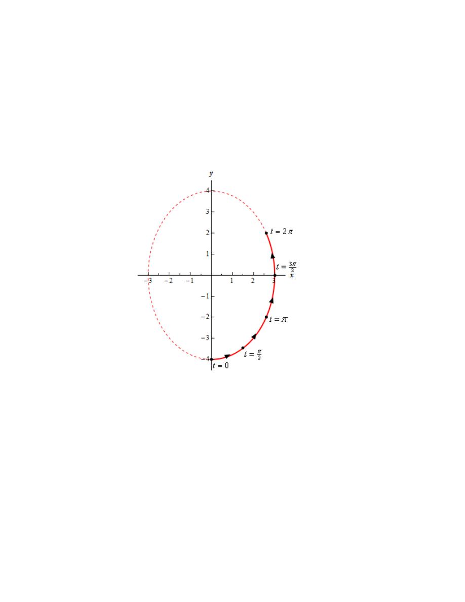
Finally, here is a sketch of the parametric curve for this set of parametric equations.

For this sketch we included a set of t’s to illustrate a handful of points and their corresponding values of
t’s. For some practice you might want to follow the analysis from Step 4 to see if you can verify the
values of t for the other three points on the graph. It would, of course, be easier to just plug them in to
verify, but the practice would of the Step 4 analysis might be useful to you.

Note as well that we included the full sketch of the ellipse as a dashed graph to help illustrate the portion
of the ellipse that the parametric curve is actually covering.

Also, because the problem asked for it here are the formal limits on x and y for this parametric curve.

≤ ≤

− ≤ ≤

You should also take a look at problems 4 and 5 in this section and contrast the number of traces of the
curve with this problem. The only difference in the set of parametric equations in problems 4, 5 and 6 is
the argument of the trig functions. After going through these three problems can you reach any
conclusions on how the argument of the trig functions will affect the parametric curves for this type of
parametric equations?

Calculus II

http://tutorial.math.lamar.edu/terms.aspx

7.The path of a particle is given by the following set of parametric equations. Completely describe the
path of the particle. To completely describe the path of the particle you will need to provide the following
information.
(i) A sketch of the parametric curve (including direction of motion) based on the equation you get by
eliminating the parameter.
(ii) Limits on x and y.
(iii) A range of t’s for a single trace of the parametric curve.
(iv) The number of traces of the curve the particle makes if an overall range of t’s is provided in the
problem.

( )

3 2 cos 3

1 4 sin 3

= −

= +

Step 1
There’s a lot of information we’ll need to find to fully answer this problem. However, for most of it we
can follow the same basic ordering of steps we used for the first few problems in this section.  We will
need however to do a little extra work along the way.

Also, because most of the work here is similar to the work we did in Problems 4 – 6 of this section we
won’t be putting in as much explanation to a lot of the work we’re doing here. So, if you need some
explanation for some of the work you should go back to those problems and check the corresponding
steps.

First we’ll eliminate the parameter from this set of parametric equations. For this particular set of
parametric equations we will make use of the well-known trig identity,

( )

cos

sin

We can solve each of the parametric equations for sine and cosine as follows,

( )

cos 3

sin 3

−

Plugging these into the trig identity gives,

(

) (

)

−









⇒









−









Therefore, the parametric curve will be some or all of the graph of this ellipse.

Step 2

At this point let’s get our first guess as to the limits on x and y. As noted in previous problems
what we’re really finding here is the largest possible ranges for x and y. In later steps we’ll
determine if this the actual set of limits on x and y or if we have smaller ranges.

We can use our knowledge of sine and cosine to determine the limits on x and y as follows,

Calculus II

http://tutorial.math.lamar.edu/terms.aspx

( )

1 cos 3

1 sin 3

2 cos 3

4 sin 3

3 2 cos 3

3 1 4 sin 3

− ≤

≤

− ≤

≤

≥ −

− ≤

≤

≥ −

≥

− ≤ +

≤

≤ ≤

− ≤ ≤

Remember that all we need to do is start with the appropriate trig function and then build up the equation
for x and y by first multiplying the trig function by any coefficient, if present, and then adding/subtracting
any numbers that might be present.  We now have the largest possible set of limits for x and y.

This problem does not have a range of t’s that might restrict how much of the parametric curve gets
sketched out.  This means that the parametric curve will be fully traced out.

Remember that when we talk about the parametric curve getting fully traced out this doesn’t, in general,
mean the full ellipse we found in Step 1 gets traced out by the parametric equation. All “fully traced out”
means, in general, is that whatever portion of the ellipse that is described by the set of parametric curves
will be completely traced out.

However, for this problem let’s also note as well that the ranges for x and y we found above also
correspond the maximum ranges for x and y we get from the equation of the ellipse we found in Step 1.
This means that, for this problem, the ellipse will get fully traced out at least once by the parametric curve
and so these are the full limits on x and y.

Step 3
Let’s next get the direction of motion for the parametric curve.

Let’s use

as a “starting” point for this analysis. At

we are at the point

( )

1,1

. If we increase t

we can see that both x and y must increase until we get to the point

( )

3, 5

. Increasing t further from this

point will force x to continue to increase, but y will now start to decrease until we reach the point

( )

5,1

Next, when we increase t further both x and y will decrease until we reach the point

(

)

3, 3

−

. Finally,

increasing t even more we get x continuing to decrease while y starts to increase until we get back to

( )

1,1

, the point we “started” the analysis at.

We didn’t put a lot of “explanation into this but if you think about the parametric equations and how
sine/cosine behave as you increase t you should see what’s going on. In the x equation we see that the
coefficient of the cosine is negative and so if cosine increases x must decrease and if cosine decreases x
must increase. For the y equation the coefficient of the sine is positive and so both y and sine will
increase or decrease at the same time.

Okay, in all of the analysis above we must be moving in a clockwise direction.  Also, note that because of
the oscillating nature of sine and cosine once we reach back to the “starting” point the behavior will
simply repeat itself.  This in turn tells us that once we arrive back at the “starting” point we will continue
to trace out the parametric curve in a clockwise direction.

Step 4

Calculus II

http://tutorial.math.lamar.edu/terms.aspx

From the analysis in the last step we saw that without any range of t’s restricting the parametric curve,
which we don’t have here, the parametric curve will completely trace out the ellipse that we found in Step
1.

Therefore, the next thing we should do is determine a range of t’s that it will take to complete one trace of
the parametric curve. Note that one trace of the parametric curve means that no portion of the parametric
curve will ever be retraced. For this problem that means we trace out the ellipse exactly once.

So, as with the last step let’s “start” at the point

( )

1,1

, which corresponds to

. So, the next question

to ask is what value of

will we reach this point again.

In order to be at the point

( )

1,1

we need to require that

( )

cos 3

and

( )

sin 3

. So, for

know we’ll have

( )

cos 3

2 , 4 , 6 ,

π π π



and we’ll have

( )

sin 3

, 2 , 3 ,

π π π



The first value of t that is in both of these lists is

. So, we’ll get back to the “starting” point at,

⇒

Therefore, one trace will be completed in the range,

≤ ≤

Note that this is only one possible answer here. Any range of t’s with a “net” range of

t’s, with the

endpoints of the t range corresponding to start/end points of the parametric equation, will work. So, for
example, any of the following ranges of t’s would also work.

−

≤ ≤

− ≤ ≤

There are of course many other possible ranges of t’s for a one trace. Note however, as the last example
above shows, because the full ellipse is traced out, each range doesn’t all need to start/end at the same

place. The range we originally arrived at as well as the first two ranges above all start/end at

( )

1,1

while

the third range above starts/ends at

( )

5,1

Step 5
Now that we have a range of t’s for one full trace of the parametric curve we could determine the number
of traces the particle makes. However, because we weren’t given an overall range of t’s we can’t do that
for this problem.

Step 6
Finally, here is a sketch of the parametric curve for this set of parametric equations.

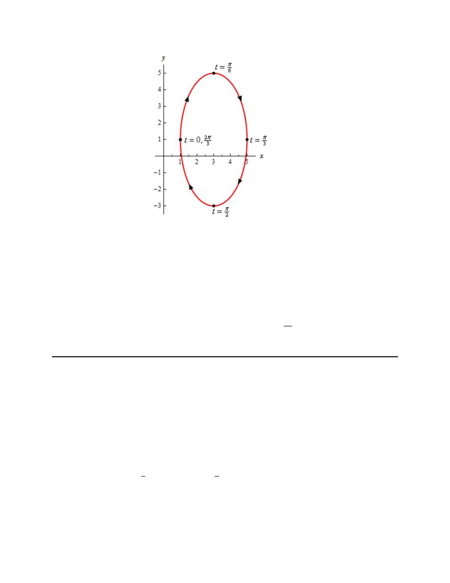
Calculus II

http://tutorial.math.lamar.edu/terms.aspx

For this sketch we included a set of t’s to illustrate where the particle is at while tracing out of the curve.
For some practice you might want to follow the analysis from Step 4 to see if you can verify the values of
t for the other three points on the graph. It would, of course, be easier to just plug them in to verify, but
the practice would of the Step 4 analysis might be useful to you.

Here is also the formal answers for all the rest of the information that problem asked for.

Range of :

Range of for one trace :

Total number of traces :

n/a

≤ ≤

− ≤ ≤

≤ ≤

8.The path of a particle is given by the following set of parametric equations. Completely describe the
path of the particle. To completely describe the path of the particle you will need to provide the following
information.
(i) A sketch of the parametric curve (including direction of motion) based on the equation you get by
eliminating the parameter.
(ii) Limits on x and y.
(iii) A range of t’s for a single trace of the parametric curve.
(iv) The number of traces of the curve the particle makes if an overall range of t’s is provided in the
problem.

( )

4 sin

1 2 cos

= −

−

≤ ≤

Calculus II

http://tutorial.math.lamar.edu/terms.aspx

Also, because most of the work here is similar to the work we did in Problems 4 – 6 of this section we
won’t be putting in as much explanation to a lot of the work we’re doing here. So, if you need some
explanation for some of the work you should go back to those problems and check the corresponding
steps.

First we’ll eliminate the parameter from this set of parametric equations. For this particular set of
parametric equations we will make use of the well-known trig identity,

( )

cos

sin

We can solve each of the parametric equations for sine and cosine as follows,

( )

sin

cos

−

Plugging these into the trig identity gives,

−

 

⇒

−

 

−

 

Therefore, with a little algebraic manipulation, we see that the parametric curve will be some or all of the
parabola above. Note that while many parametric equations involving sines and cosines are some or all of
an ellipse they won’t all be as this problem shows. Do not get so locked into ellipses when seeing
sines/cosines that you always just assume the curve will be an ellipse.

Step 2

We can use our knowledge of sine and cosine to determine the limits on x and y as follows,

( )

( )
( )

1
4

1 sin

1 cos

4 sin

cos

2 cos

1 1 2 cos

− ≤

≤

− ≤

≤

− ≤

≤

− ≤ ≤

≥ −

− ≤ ≤

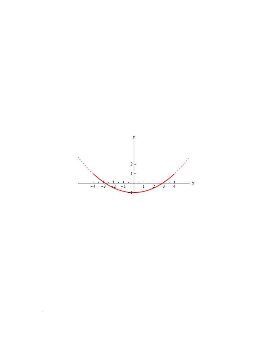
Calculus II

http://tutorial.math.lamar.edu/terms.aspx

problem statement. It is always possible that the parametric curve will not trace out a full trace in the
given range of t’s. In a later step we’ll determine if the parametric curve does trace out a full trace and
hence determine the actual limits on x and y.

Remember that when we talk about the parametric curve getting fully traced out this doesn’t, in general,
mean the full parabola we found in Step 1 gets traced out by the parametric equation. All “fully traced
out” means, in general, is that whatever portion of the parabola that is described by the set of parametric
curves will be completely traced out.

In fact, for this problem, we can see that the parabola from Step 1 will not get fully traced out by the
particle regardless of any range of t’s. The largest possible portion of the parabola that can be traced out
by the particle is the portion that lies in the range of x and y given above. In a later step we’ll determine if
the largest possible portion of the parabola does get traced out or if the particle only traces out part of it.

Step 3
Let’s next get the direction of motion for the parametric curve. For this analysis it might be useful to
have a quick sketch of the largest possible parametric curve. So, here is a quick sketch of that.

The dashed line is the graph of the full parabola from Step 1 and the solid line is the portion that falls into
our largest possible range of x and y we found in Step 2. As an aside here note that the two ranges are
complimentary. In other words, if we sketch the graph only for the range of x we automatically get the
range for y. Likewise, if we sketch the graph only for the range of y we automatically get the range for x.
This is a good check for your graph. The x and y ranges should always match up!

When our parametric curve was an ellipse (the previous problem for example) no matter what point we
started the analysis at the curve would eventually trace out around the ellipse and end up back at the
starting point without ever going back over any portion of itself. The main issue we faced with the ellipse
problem was we could rotate around the ellipse in a clockwise or a counter clockwise motion to do this
and a careful analysis of the behavior of both the x and y parametric equations was required to determine
just which direction we were going.

With a parabola for our parametric curve things work a lot differently. Let’s suppose that we “started” at
the right end point (this is just randomly picked for no other reason that I’m right handed so don’t think
there is anything special about this point!) and it doesn’t matter what t we use to get to that point.

At this point we know that we are at

and in order for x to have that value we must also have

( )

1
4

sin

. Now, as we increase t from this point (again it doesn’t matter just what the value of t is) the

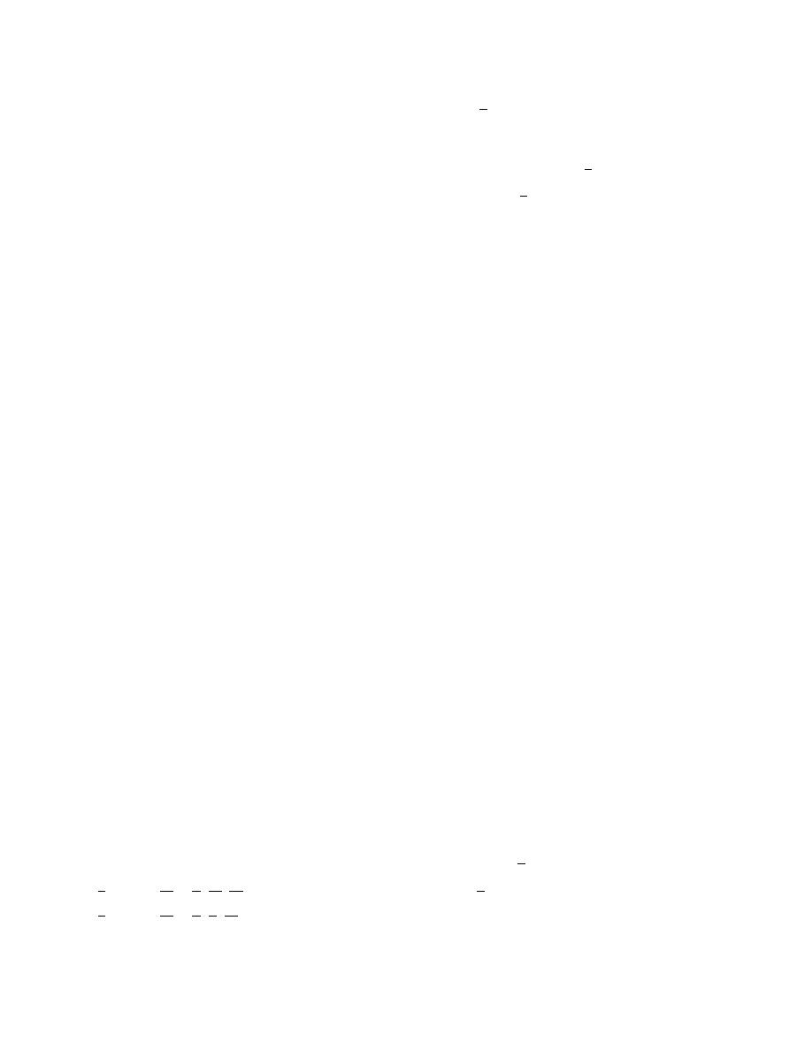
Calculus II

http://tutorial.math.lamar.edu/terms.aspx

only option for sine is for it to decrease until it has the value

( )

1
4

sin

= −

. This in turn means that if we

start at the right end point we have no option but to proceed along the curve going to the left.

However, we don’t just reach the left end point and then stop! Once we are at

( )

1
4

sin

= −

if we further

increase t we know that sine will also increase until it has the value

( )

1
4

sin

and so we must move

back along the curve to the right until we are back at the right end point.

Unlike the ellipse however, the only way for this to happen is for the particle to go back over the parabola
moving in a rightward direction. Remember that the particle moves to the right or left it must trace out a
portion of the parabola that we found in Step 1! Any particle traveling along the path given by the set of
parametric equations must follow the graph of the parabola and never leave it.

In other words, if we don’t put any restrictions on t a particle on this parametric curve will simply
oscillate left and right along the portion of the parabola sketched out above. In this case however we do
have a range of t’s so we’ll need to determine a range of t’s for one trace to fully know the direction of
motion information of the particle on this path and we’ll do that in the next step. With a restriction on the
range of t’s it is possible that the particle won’t make a full trace or it might retrace some or all of the
curve so we can’t say anything definite about the direction of motion for the particle over the full range of
t’s until the next step when we determine a range of t’s for one full trace of the curve.

Before we move on to the next step there is a quick topic we should address. We only used the x equation
to do this analysis and never addressed the y-equation anywhere in the analysis. It doesn’t really matter
which one we use as both will give the same information.

Step 4
Now we need to determine a range of t’s for one full trace of the parametric curve. It is important for this
step to remember that one full trace of the parametric curve means that no portion of the parametric curve
can be retraced.

Note that one full trace does not mean that we get back to the “starting” point. When we dealt with an
ellipse in the previous problem that was one trace because we did not need to retrace any portion of the
ellipse to get back to the starting point. However, as we saw in the previous step that for our parabola
here we would have to retrace the full curve to get back to the starting point.

So, one full trace of the parametric curve means we move from the right end point to the left end point
only or visa-versa and move from the left end point to the right end point.  Which direction we move
doesn’t really matter here so let’s get a range of t’s that take us from the left end point to the right end
point.

In all the previous problems we’ve used

as our “starting” point but that won’t work for this problem

because that actually corresponds to the vertex of the parabola. We want to start at the left end point so
the first part of this process is actually determine a t that will put us at the left end point.

In order to be at the left end point,

(

)

4,1

−

, we need to require that

( )

1
4

sin

= −

which occurs if

1
4

−



. We also need to require that

( )

1
4

cos

which occurs if

1
4

, ,

π π

−



. There are going to be many numbers that are in both lists here so all we

need to do is pick one and proceed. From the numbers that we’ve listed here we could use either

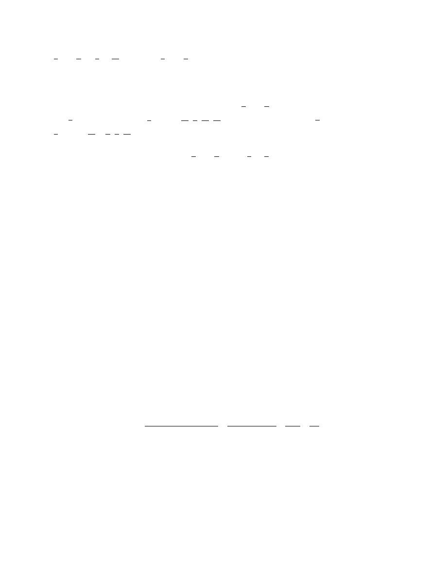
Calculus II

http://tutorial.math.lamar.edu/terms.aspx

1
4

= −

1
4

. We’ll use

1
4

= −

, i.e. when

= −

, simply because it is the first one that

occurs in both lists. Therefore we will be at the left end point when

= −

Let’s now move to the right end point,

( )

4,1

. In order to get the range of t’s for one trace this means

we’ll need the next t with

> −

(which corresponds to

1
4

> −

). To do this we need to require that

( )

1
4

sin

which occurs if

1
4

, ,

π π

−



and we need to that

( )

1
4

cos

which occurs if

1
4

, ,

π π

−



. .

The first t that is in both of these lists with

1
4

> −

is then

1
4

, i.e. when

. So, the first t

after

= −

that puts us at the right end point is

. This means that a range of t’s for one full

trace of the parametric curve is then,

−

≤ ≤

Note that this is only one possible answer here. Any range of t’s with a “net” range of

(

)

− −

t’s, with the endpoints of the t range corresponding to start/end points of the parametric curve, will work.
So, for example, any of the following ranges of t’s would also work.

−

≤ ≤ −

≤ ≤

The direction of motion for each may be different range of t’s of course. Some will trace out the curve
moving from left to right while others will trace out the curve moving from right to left. Because the
problem did not specify a particular direction any would work.

Note as well that the range

−

≤ ≤

falls completely inside the given range of t’s specified in the

problem and so we know that the particle will trace out the curve more than once over the full range of
t’s.  Determining just how many times it traces over the curve will be determined in the next step.

Step 5
Now that we have a range of t’s for one full trace of the parametric curve we can determine the number of
traces the particle makes.

This is a really easy step.  We know the total time the particle was traveling and we know how long it
takes for a single trace.  Therefore,

(

)

(

)

Total Time Traveled

Number Traces =

21.5 traces

Time for One Trace

− −

Step 6
Finally, here is a sketch of the parametric curve for this set of parametric equations.

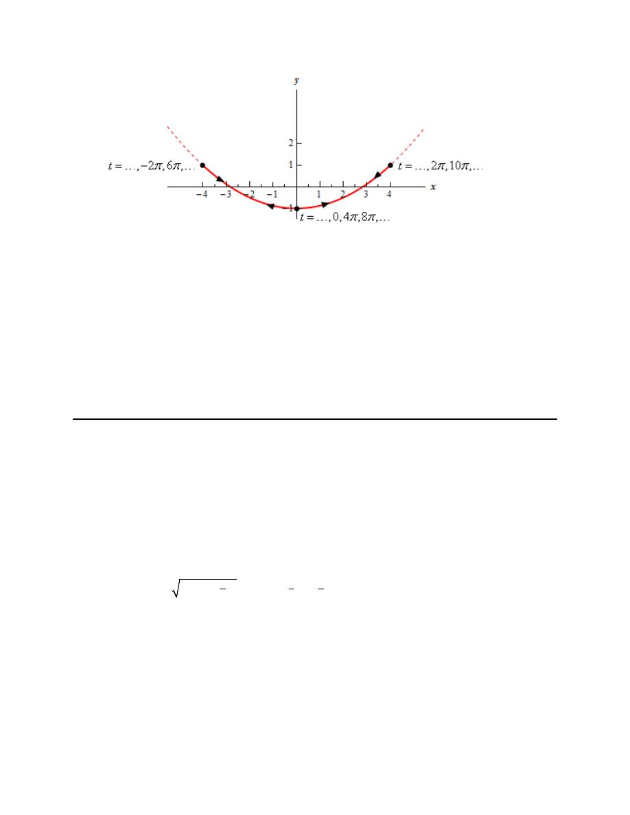
Calculus II

http://tutorial.math.lamar.edu/terms.aspx

For this sketch we indicated the direction of motion by putting arrow heads going both directions in
places on the curve. We also included a set of t’s for a couple of points to illustrate where the particle is
at while tracing out of the curve. The dashed line is the continuation of the parabola from Step 1 to
illustrate that our parametric curve is only a part of the parabola.

Here is also the formal answers for all the rest of the information that problem asked for.

Range of :

Range of for one trace :

Total number of traces :

21.5

− ≤ ≤
− ≤ ≤

−

≤ ≤

9.The path of a particle is given by the following set of parametric equations. Completely describe the
path of the particle. To completely describe the path of the particle you will need to provide the following
information.
(i) A sketch of the parametric curve (including direction of motion) based on the equation you get by
eliminating the parameter.
(ii) Limits on x and y.
(iii) A range of t’s for a single trace of the parametric curve.
(iv) The number of traces of the curve the particle makes if an overall range of t’s is provided in the
problem.

( )

4 cos

cos

= +

−

≤ ≤

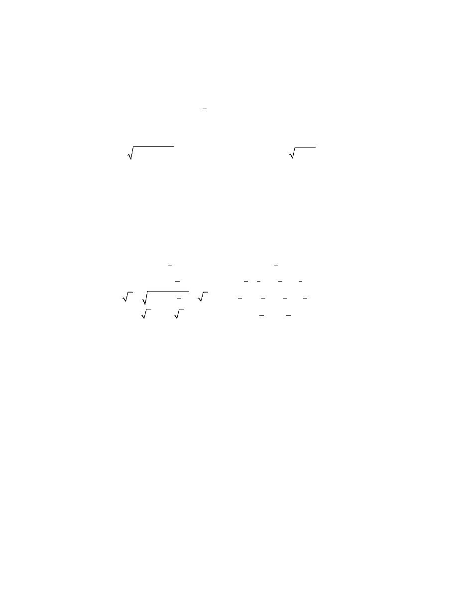
Calculus II

http://tutorial.math.lamar.edu/terms.aspx

First we’ll eliminate the parameter from this set of parametric equations. For this particular set of
parametric equations notice that we can quickly and easily eliminate the parameter simply by solving the
y equation for cosine as follows,

( )

5
2

cos

−

Plugging this into the cosine in the x equation gives,

(

)

1 3

−

⇒

So, the parametric curve will be some or all of the graph of this square root function.

Step 2

We can use our knowledge of cosine to determine the limits on x and y as follows,

( )

cos

4 cos

cos

4 cos

cos

− ≤

≤

− ≤

≤

≤ +

≤

− ≤

≤

≤ +

≤

≤ ≤

Remember that all we need to do is start with the cosine and then build up the equation for x and y by first
multiplying the trig function by any coefficient, if present, and then adding/subtracting any numbers that
might be present.  We now have the largest possible set of limits for x and y.

Now, at this point we need to be a little careful.  As noted above what we’ve actually found here are the
largest possible ranges for the limits on x and y.  This set of inequalities for the limits on x and y assume
that the parametric curve will be fully traced out at least once for the range of t’s we were given in the
problem statement. It is always possible that the parametric curve will not trace out a full trace in the
given range of t’s. In a later step we’ll determine if the parametric curve does trace out a full trace and
hence determine the actual limits on x and y.

Remember that when we talk about the parametric curve getting fully traced out this doesn’t, in general,
mean the full square root graph we found in Step 1 gets traced out by the parametric equation. All “fully
traced out” means, in general, is that whatever portion of the square root graph that is described by the set
of parametric curves will be completely traced out.

In fact, for this problem, we can see that the square root from Step 1 will not get fully traced out by the
particle regardless of any range of t’s. The largest possible portion of the square root graph that can be
traced out by the particle is the portion that lies in the range of x and y given above. In a later step we’ll
determine if the largest possible portion of the square root graph does get traced out or if the particle only
traces out part of it.

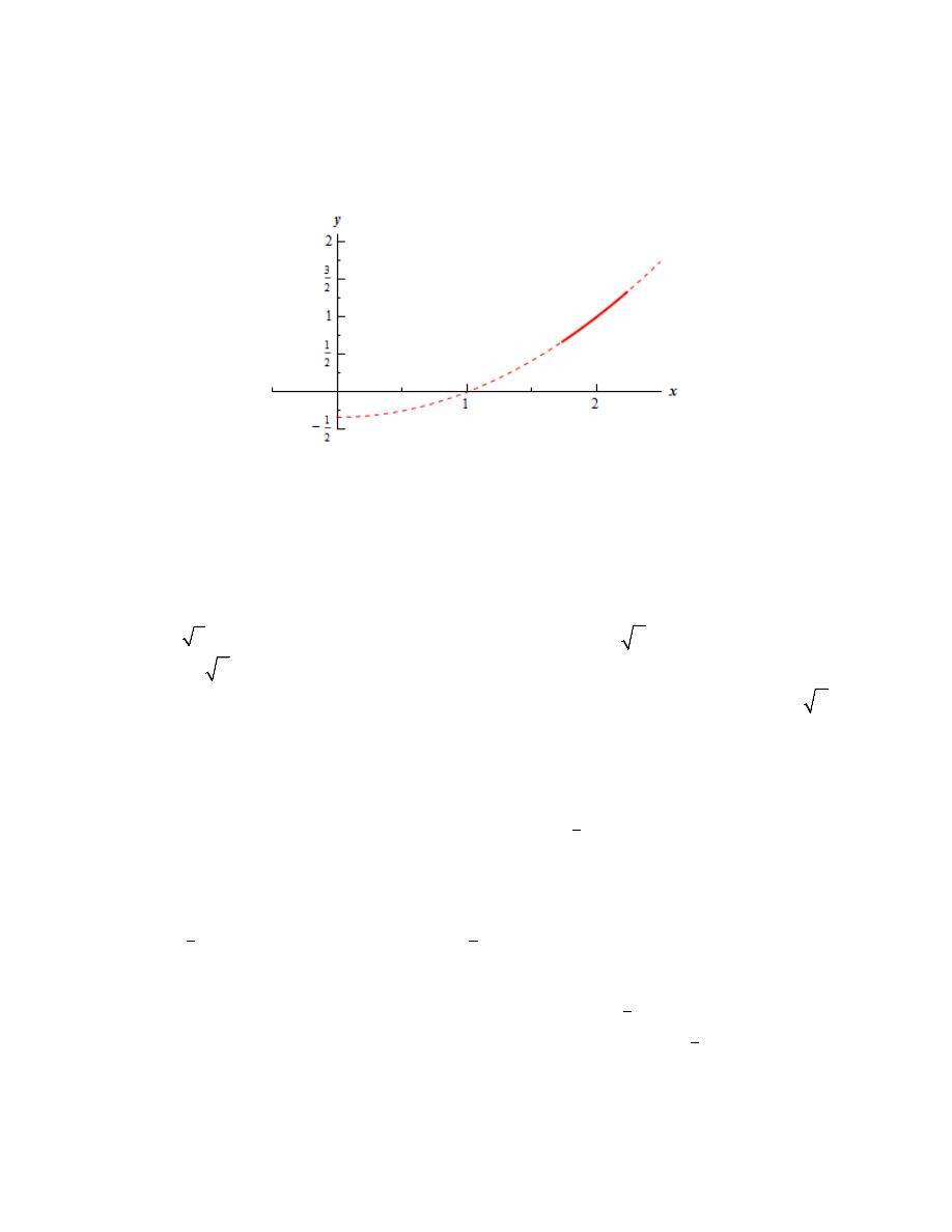
Calculus II

http://tutorial.math.lamar.edu/terms.aspx

Step 3
Let’s next get the direction of motion for the parametric curve. For this analysis it might be useful to
have a quick sketch of the largest possible parametric curve. So, here is a quick sketch of that.

The dashed line is the graph of the full square root from Step 1 and the solid line is the portion that falls
into our largest possible range of x and y we found in Step 2. As an aside here note that the two ranges
are complimentary. In other words, if we sketch the graph only for the range of x we automatically get
the range for y. Likewise, if we sketch the graph only for the range of y we automatically get the range
for x. This is a good check for your graph. The x and y ranges should always match up!

Before moving on let’s address the fact that is doesn’t look like square root graphs that most of us are
used to seeing. Keep in mind that the typical square root function that we’re used to working at is in the

form

. Our equation for this problem however is in the form

. If you think about it the

graph of

is nothing more than the portion of the graph of

corresponding to

≥

(recall

square roots only return positive or zero values!). Of course the function for this problem is not

but it is similar enough that the ideas discussed here are still valid just for a slightly different function.

Okay, let’s get back to the problem.

This problem is going to be a lot like the previous problem in terms of direction of motion. First note that

if we start at the lower left hand point we need to require that

( )

5
2

cos

= −

since that is the only way for

both x and y to have their minimal values (which puts us at the lower left hand point)! It also doesn’t
matter what value of t we use at this point. All that matters is that we are at the lower left hand point.

If we now increase t (from whatever “starting” value we had) we know that cosine will need to increase

from

( )

5
2

cos

= −

until it reaches a value of

( )

5
2

cos

. By looking at the parametric equations we

can see that this will also force both x and y to increase until it reaches the upper right hand point.

Now, the graph won’t just stop here. Once cosine reaches a value of

( )

5
2

cos

we know that

continuing to increase t will now cause cosine to decrease it reaches a value of

( )

5
2

cos

= −

. This in

turn forces both x and y to decrease until it once again reaches the lower left hand point.

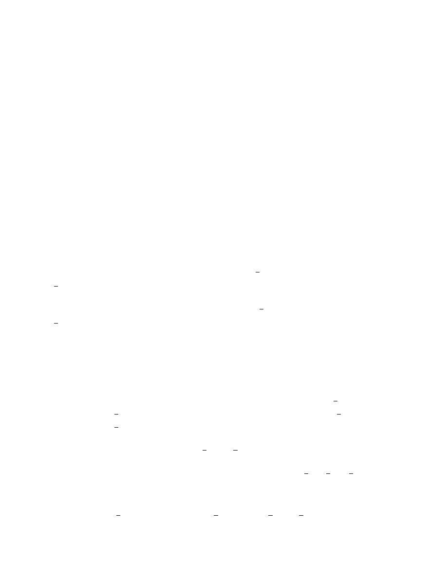
Calculus II

http://tutorial.math.lamar.edu/terms.aspx

In other words, if we don’t put any restrictions on t a particle on this parametric curve will simply
oscillate left and right along the portion of the square root sketched out above. In this case however we
do have a range of t’s so we’ll need to determine a range of t’s for one trace to fully know the direction of
motion information of the particle on this path and we’ll do that in the next step. With a restriction on the
range of t’s it is possible that the particle won’t make a full trace or it might retrace some or all of the
curve so we can’t say anything definite about the direction of motion for the particle over the full range of
t’s until the next step when we determine a range of t’s for one full trace of the curve.

Step 4
Now we need to determine a range of t’s for one full trace of the parametric curve. It is important for this
step to remember that one full trace of the parametric curve means that no portion of the parametric curve
can be retraced.

Note that one full trace does not mean that we get back to the “starting” point. When we dealt with an
ellipse in a previous problem that was one trace because we did not need to retrace any portion of the
ellipse to get back to the starting point. However, as we saw in the previous step that for our square root
here we would have to retrace the full curve to get back to the starting point.

So, one full trace of the parametric curve means we move from the right end point to the left end point
only or visa-versa and move from the left end point to the right end point.  Which direction we move
doesn’t really matter here so let’s get a range of t’s that take us from the left end point to the right end
point.

In order to be at the left end point we need to require that

( )

5
2

cos

= −

which occurs if

5
2

, 3 ,

, , 3 ,

π π π π

−



. Note as well that unlike the previous problems, which had both sine and

cosine, this set of parametric equations has only cosine and so all we need to do here is look at this. Also,

in order to be at the right end point we need to require that

( )

5
2

cos

which occurs if

5
2

, 4 , 2 , 0, 2 , 4 ,

π π

−



So, if we want to move from the left to right all we need to do is chose one from the list of t’s
corresponding to the left end point and then first t that comes that from the list corresponding to the right
end point and we’ll have a range of t’s for one trace. To move from the right to left we just go the
opposite direction, i.e. chose a t from the right end point list and then take the first t after that from the left
end point list.

So, for this problem, since we said we were going to move from left to right, we’ll use

5
2

, which

corresponds to

2
5

, for the left end point. That in turn means that we’ll need to use

5
2

, which

corresponds to

4
5

, for the right end point. That means the range of t’s for one trace is,

≤ ≤

This is only one possible answer here. Any range of t’s with a “net” range of

( )

−

t’s, with

the endpoints of the t range corresponding to start/end points of the parametric curve, will work. So, for
example, any of the following ranges of t’s would also work.

−

≤ ≤

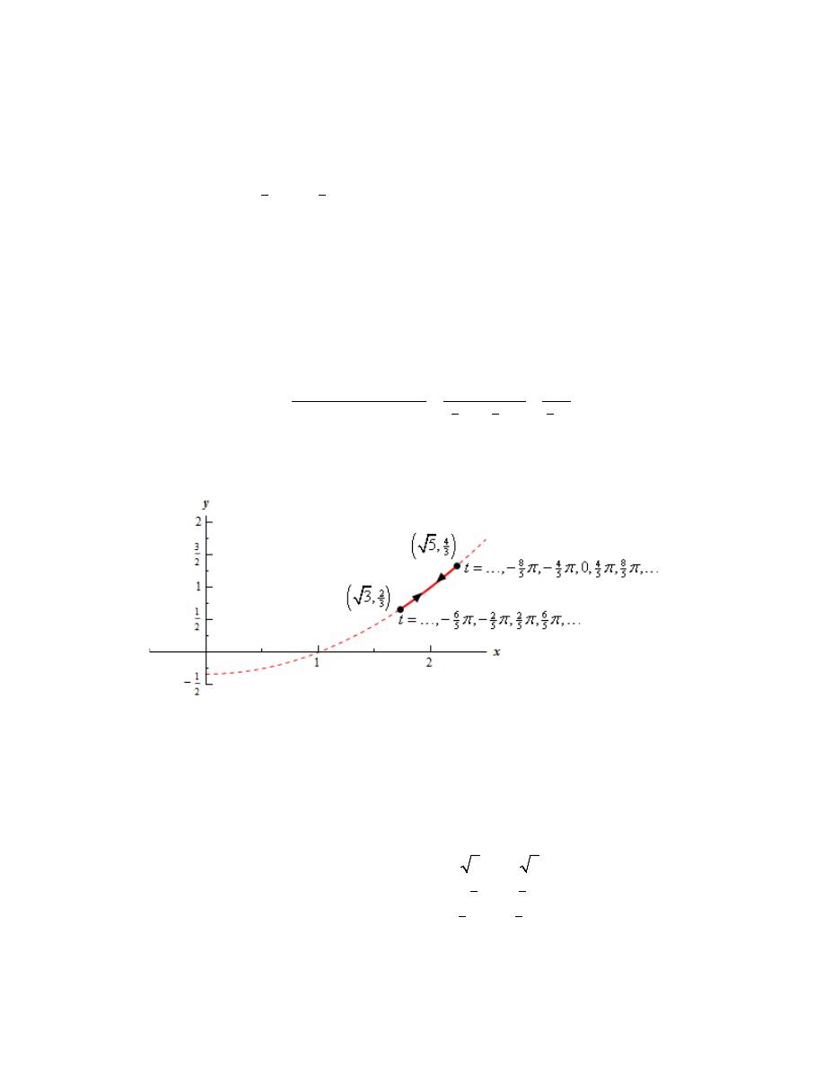
Calculus II

http://tutorial.math.lamar.edu/terms.aspx

Note as well that the range

≤ ≤

falls completely inside the given range of t’s specified in the

(

)

( )

Total Time Traveled

Number Traces =

125 traces

Time for One Trace

− −

−

Step 6
Finally, here is a sketch of the parametric curve for this set of parametric equations.

For this sketch we indicated the direction of motion by putting arrow heads going both directions in
places on the curve. We also included a set of t’s for a couple of points to illustrate where the particle is
at while tracing out of the curve as well as coordinates for the end points since they aren’t “nice” points..
The dashed line is the continuation of the square root from Step 1 to illustrate that our parametric curve is
only a part of the square root.

Here is also the formal answers for all the rest of the information that problem asked for.

Range of :

Range of for one trace :

Total number of traces :

125

≤ ≤

Calculus II

http://tutorial.math.lamar.edu/terms.aspx

10.The path of a particle is given by the following set of parametric equations. Completely describe the
path of the particle. To completely describe the path of the particle you will need to provide the following
information.
(i) A sketch of the parametric curve (including direction of motion) based on the equation you get by
eliminating the parameter.
(ii) Limits on x and y.
(iii) A range of t’s for a single trace of the parametric curve.
(iv) The number of traces of the curve the particle makes if an overall range of t’s is provided in the
problem.

(

)

3
4

cos 1

≤ ≤

1
2

Now, just recall that

( )

and so we can plug the above equation into the exponential in the y

equation to get,

(

)

( )

(

)

( )

(

)

(

)

cos 1

So, the parametric curve will be some or all of the graph of this cosine function.

Step 2

At this point let’s work on the limits for x and y. In this case, unlike most of the previous
problems, things will work a little differently.

Let’s start by noting that unlike sine and cosine functions we know

is always an increasing function

(you can do some quick Calculus I work to verify this right?).

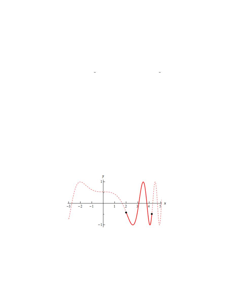
Calculus II

http://tutorial.math.lamar.edu/terms.aspx

Why do we care about this? Well first the x equation is just a constant times

and we are given a range

of t’s for the problem. Next, the fact that

is an increasing function means that the x equation,

= e

is also an increasing function (because the 2 is positive). Therefore, the smallest value of x will occur at
the smallest value of t in the range of t’s. Likewise, the largest value of x will occur at the largest value of
t in the range of t’s.

Therefore, the range of x for our parametric curve is,

≤ ≤

⇒

≤ ≤

Unlike the previous problems where we usually needed to do a little more verification work we know at
this point that this is the range of x’s.

For the range of y’s we will need to do a little work to get the correct range of y’s but it won’t be as much
extra work as in previous problems and we can do it all in this step. First let’s notice that because the y

equation is in the form of

( )

cos



. The argument of the cosine doesn’t matter for the first part of

the work and so wasn’t included here.

From the behavior of cosine we then know that the largest possible range of y would then be,

− ≤ ≤

Now, depending on just what values the argument of the cosine in the y equation takes over the give range
of t’s we may or may not cover this full range of values. We could do some work analyzing the argument
of the cosine to figure that out if it does cover this full range. However, there is a really easy way to
figure that if the full range is covered in this case.

Let’s just sketch the graph and see what we get. Here is a quick sketch of the graph.

Given the “messy” nature of the argument of the cosine it’s probably best to use some form of
computational aid to get the graph. The dotted portion of the graph is full graph of the function on

− ≤ ≤

without regards to the actual restriction on t. The solid portion of the graph is the portion that

corresponds to the range of t’s we were given in the problem.

From this graph we can see that the range of y’ is in fact

− ≤ ≤

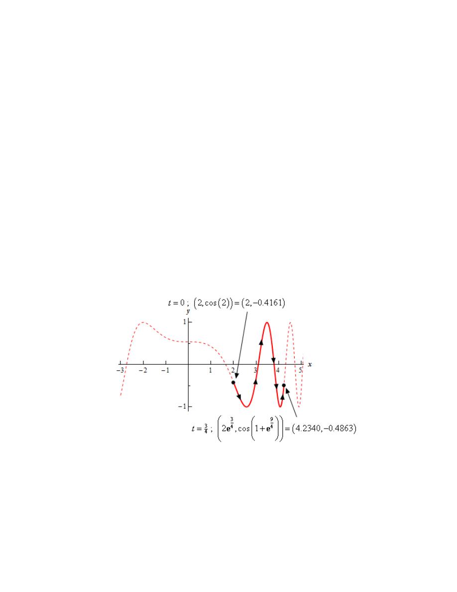
Calculus II

http://tutorial.math.lamar.edu/terms.aspx

Before proceeding with the direction of motion let’s note that we could also have just graphed the curve
in many of the previous problems to determine if the work in this step was the actual range or not.  We
didn’t do that because we could determine if these ranges were correct or not when we did the direction of
motion and range of t’s for one trace analysis (which we had to do anyway) and so didn’t need to bother
with a graph in this step for those problems.

Step 3
We now need to do the direction of motion for this curve but note that we actually found the direction of
motion in the previous step.

As noted in the previous step we know that

= e

is an increasing function and so the x’s must be

increasing as t increases. Therefore the equation must be moving from left to right as the curve is traced
out over the given range of t’s.

Also note that unlike the previous problems we know that no portion of the graph will be retraced. Again,
we know the x equation is an increasing equation. If the curve were to retrace any portion we can see that
the only way to do that would be to move back from right to left which would require x to decrease and
that can’t happen.

This means that we now know as well that the graph will trace out exactly once for the given range of t’s,
which in turn tells us that the given range of t’s is also the range of t’s for a single trace.

Step 4
Now that we have all the needed information we can do a formal sketch of the graph.

As with the graph above the dotted portion of the graph is full graph of the function on

− ≤ ≤

without regards to the actual restriction on t. The solid portion of the graph is the portion that
corresponds to the range of t’s we were given in the problem. We also included the t value and
coordinates of each end point for clarity although these are often not required for many problems.

Here is also the formal answers for all the rest of the information that problem asked for.

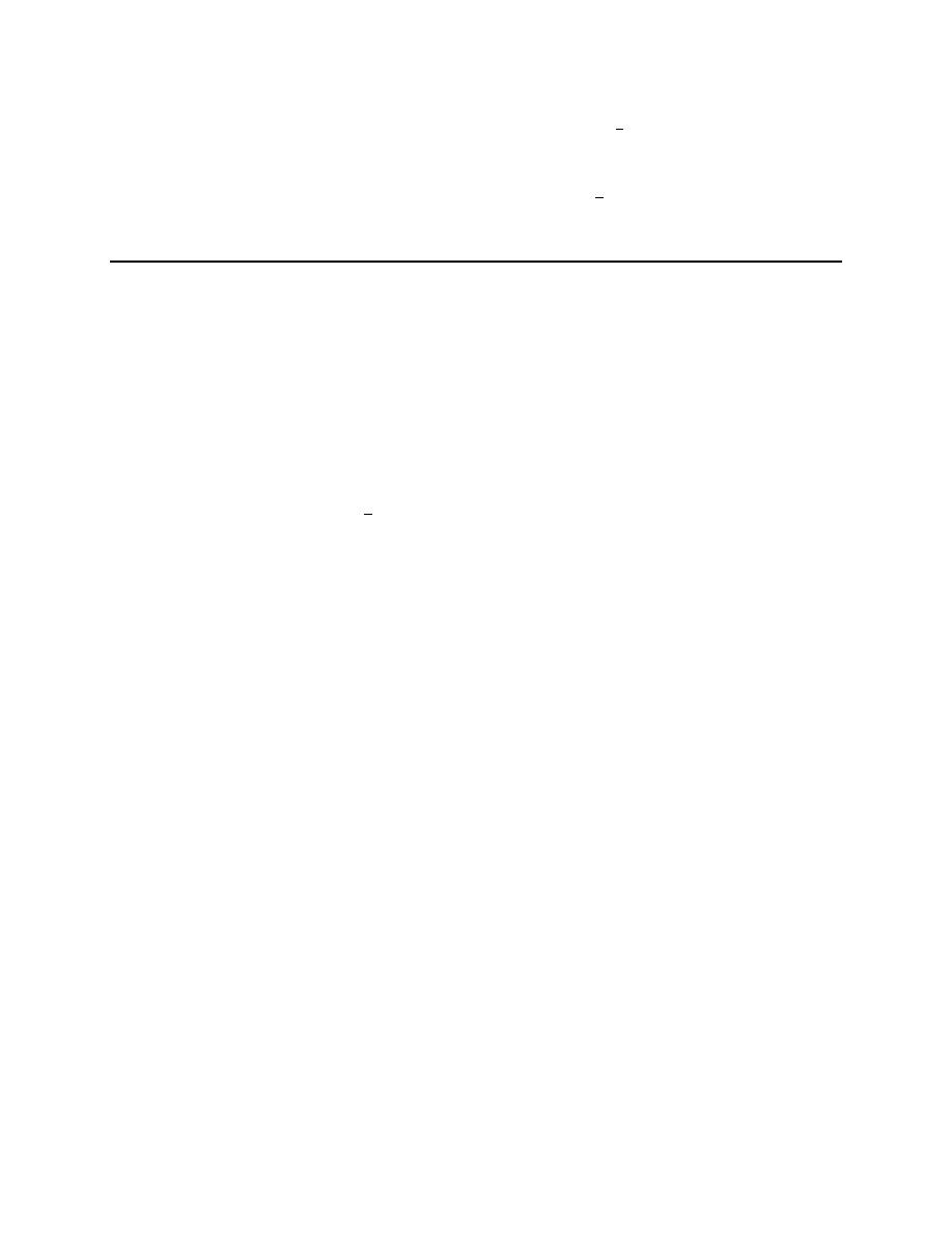
Calculus II

http://tutorial.math.lamar.edu/terms.aspx

3
4

Range of :

Range of for one trace :

Total number of traces :

≤ ≤

− ≤ ≤

≤ ≤

11.The path of a particle is given by the following set of parametric equations. Completely describe the
path of the particle. To completely describe the path of the particle you will need to provide the following
information.
(i) A sketch of the parametric curve (including direction of motion) based on the equation you get by
eliminating the parameter.
(ii) Limits on x and y.
(iii) A range of t’s for a single trace of the parametric curve.
(iv) The number of traces of the curve the particle makes if an overall range of t’s is provided in the
problem.

1
2

−

Now, just recall that

( )

−

and so we can plug the above equation into the exponential in the y

equation to get,

( )

2 2

−

− =

−

So, the parametric curve will be some or all of the graph of this quadratic function.

Step 2

At this point let’s work on the limits for x and y. In this case, unlike most of the previous
problems, things will work a little differently.

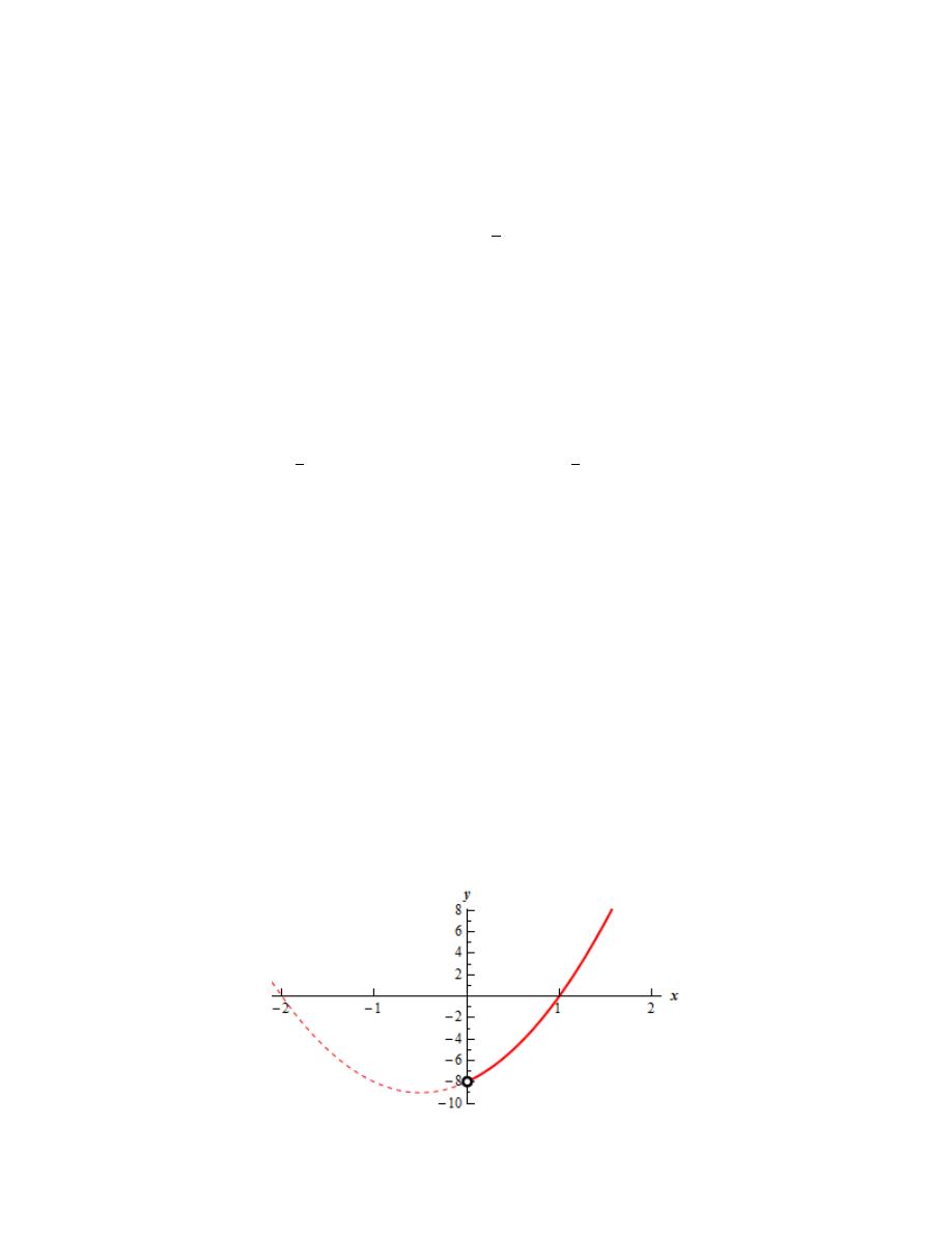
Calculus II

http://tutorial.math.lamar.edu/terms.aspx

Let’s start by noting that unlike sine and cosine functions we know

−

is always a decreasing function

as t increases (you can do some quick Calculus I work to verify this right?).

Why do we care about this? Well first the x equation is just a constant times

−

and so the fact that

−

is a decreasing function means that the x equation,

1
2

−

= e

, is also a decreasing function (because the

coefficient is positive).

Next, we aren’t given a range of t’s for this problem and so we can assume the largest possible range of
t’s. Therefore, we are safe in assuming a range of

−∞ < < ∞

for the t’s.

Now, as we’ve already noted the know that the x equation is decreasing and so the largest value of x will
occur at the left “end point” of the range. Likewise, the smallest value of x will occur at the right “end
point” of the range. For this problem both “end points” of our range are in fact infinities so we can’t just
plug in as we did in the previous problem. We can however take the following two limits.

(

)

(

)

lim

−

→ −∞

→ ∞

= ∞

From this we can see that as we approach the left end point of the t range the value of x is going to infinity
and as we approach the right end point of the t range the x value is going to zero. Note however that x can
never actually be zero because x is still defined in terms of an exponential function (which can’t be zero).
All the limit is telling us is that as we let

→ ∞

we will get

→

The range of x for our parametric curve is therefore,

< < ∞

Again, be careful with the inequalities here! We know that x can be neither zero nor infinity so we must
use strict inequalities for this range. This is something that we always need to be on the lookout for with
variable ranges of parametric equations. Depending on the parametric equations sometimes the end
points of the ranges will be strict inequalities (as with this problem) and for others they include the end
points (as with the previous problems).

For the range of y’s we will need to do a little work to get the correct range of y’s but it won’t be as much
extra work as in previous problems and we can do it all in this step. Let’s just sketch the graph and see
what we get. Here is a quick sketch of the graph.

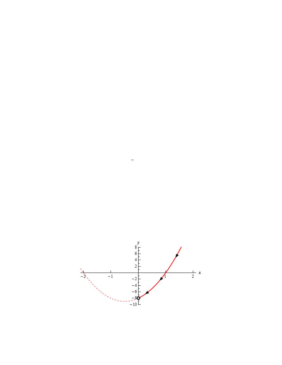
Calculus II

http://tutorial.math.lamar.edu/terms.aspx

The dotted portion of the graph is full graph of the function on

− ≤ ≤

without regards to the actual

restriction on x. The solid portion of the graph is the portion of the graph that corresponds to the
restriction on x that we found earlier in this step.

Note the “open dot” on the y-axis for the left end of the graph. This needs to be here to acknowledge that

≠

. We can also see that the y value at this point is

= −

and again we can see that for the

parametric curve we have

≠ −

Also, keep in mind that we know that

→ ∞

and so we also know that the y portion of the graph must

also continue up to infinity to match the x behavior.

So, from this quick analysis of the graph we can see that the y range for the parametric curve must be,

− < < ∞

Step 3
We now need to do the direction of motion for this curve but note that we actually found the direction of
motion in the previous step.

As noted in the previous step we know that

1
2

−

= e

is a decreasing function and so the x’s must be

decreasing as t increases.  Therefore, the equation must be moving from right to left as the curve is traced
out.

Also note that unlike most of the previous problems we know that no portion of the graph will be
retraced. Again, we know the x equation is a decreasing equation. If the curve were to retrace any
portion we can see that the only way to do that would be to move back from left to right which would
require x to increase and that can’t happen.

This means that we now know as well that the graph will trace out exactly once.

Step 4
Now that we have all the needed information we can do a formal sketch of the graph.

As with the graph above the dotted portion of the graph is full graph of the function on

− ≤ ≤

and

the solid portion of the graph is the portion that corresponds to the restrictions x and y we found in Step 2.

Calculus II

http://tutorial.math.lamar.edu/terms.aspx

Here is also the formal answers for all the rest of the information that problem asked for.

Range of :

Range of for one trace :

Total number of traces :

≤ < ∞

− ≤ < ∞

− ∞ < < ∞

12. Write down a set of parametric equations for the following equation.

(

)

ln 4

−

Solution
There really isn’t a lot to this problem. All we need to do is use the “formulas” right at the end of the
notes for this section.

A set of parametric equations for the equation above are,

(

)

ln 4

−

13. Write down a set of parametric equations for the following equation.

The parametric curve resulting from the parametric equations should be at

( )

6, 0

when

and the

curve should have a counter clockwise rotation.

Solution
If we don’t worry about the “starting” point (i.e. where the curve is at when

) and we don’t worry

about the direction of motion we know from the notes that the following set of parametric equations will
trace out a circle of radius 6 centered at the origin.

( )

6 cos

6 sin

All we need to do is verify if the extra requirements are met or not.

First, we can clearly see with a quick evaluation that when

we are at the point

( )

6, 0

as we need to

be.

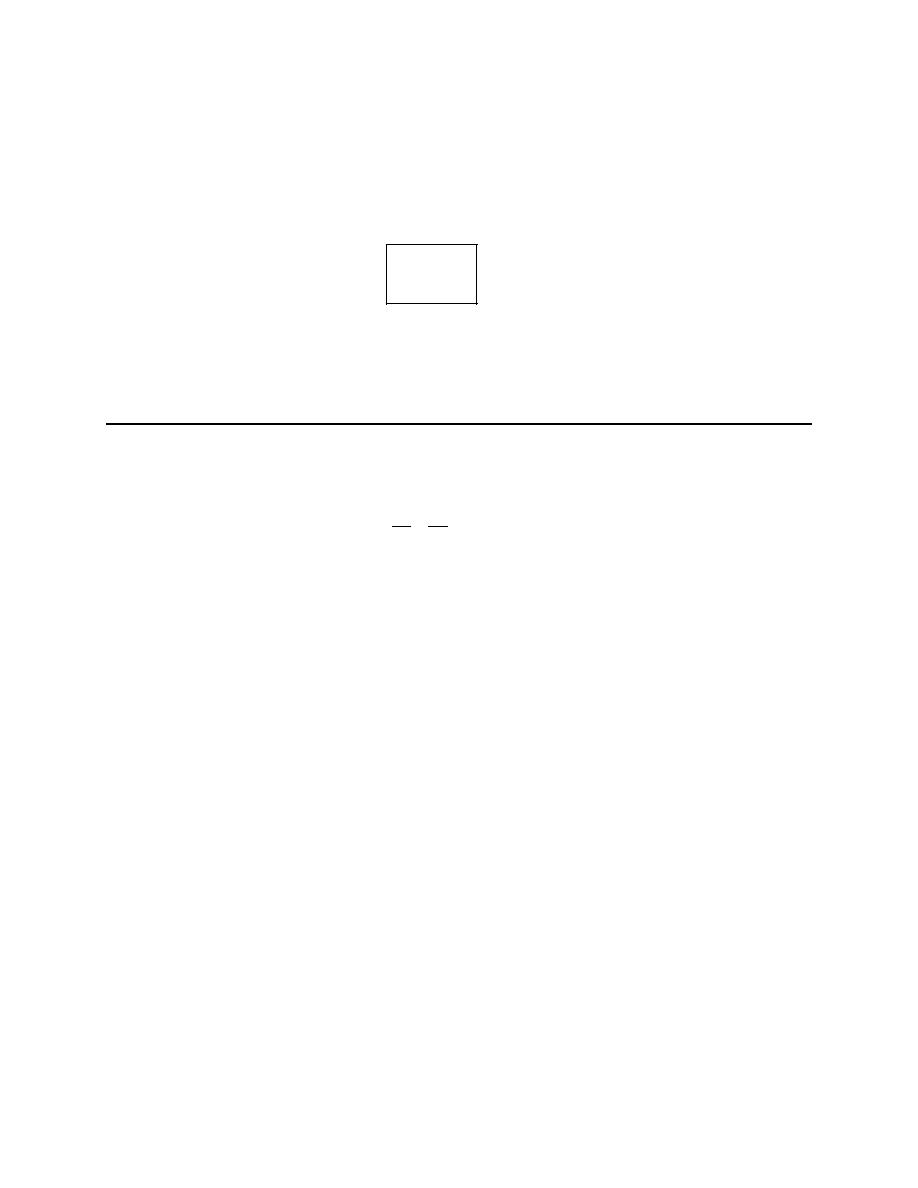
Calculus II

http://tutorial.math.lamar.edu/terms.aspx

Next, we can either use our knowledge from the examples worked in the notes for this section or an
analysis similar to some of the earlier problems in this section to verify that circles in this form will
always trace out in a counter clockwise rotation.

In other words, the set of parametric equations give above is a set of parametric equations which will
trace out the given circle with the given restrictions. So, formally the answer for this problem is,

( )

6 cos

6 sin

We’ll leave this problem with a final note about the answer here. This is possibly the “simplest” answer
we could give but it is completely possible that you may have come up with a different answer to this
problem. There are almost always lots of different possible sets of parametric equations that will trace out
a particular parametric curve according to some particular set of restrictions.

14. Write down a set of parametric equations for the following equation.

The parametric curve resulting from the parametric equations should be at

(

)

0, 7

−

when

and the

curve should have a clockwise rotation.

Solution
If we don’t worry about the “starting” point (i.e. where the curve is at when

) and we don’t worry

about the direction of motion we know from the notes that the following set of parametric equations will
trace out the ellipse given by the equation above.

( )

2 cos

7 sin

The problem with this set of parametric equations is that when

we are at the point

( )

7, 0

which is

not the point we are supposed to be at. Also, from our knowledge of the examples worked in the notes for
this section or an analysis similar to some of the earlier problems in this section we can see that the
parametric curve traced out by this set of equations will trace out in a counter clockwise rotation – again
not what we need.

So, we need to come up with a different set of parametric equations that meets the requirements.

The first thing to acknowledge is that using sine and cosine will always be the easiest way to get a set of
parametric equations for an ellipse. However, there is no reason at all to always use cosine for the x
equation and sine for the y equation.

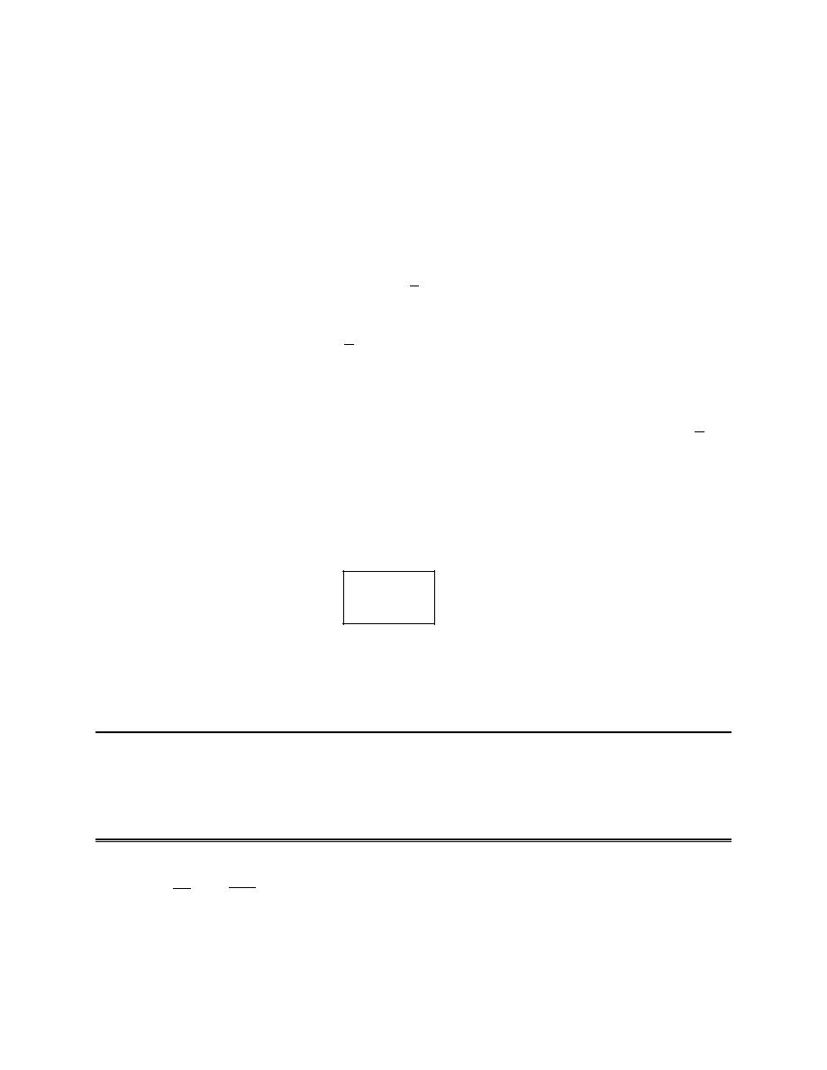
Calculus II

http://tutorial.math.lamar.edu/terms.aspx

Knowing that we need

and

= −

when

and using the fact that we know that

( )

sin 0

and

( )

cos 0

the following set of parametric equations will “start” at the correct point when

( )

2 sin

7 cos

= −

All we need to do now is check if this will trace out the ellipse in a clockwise direction.

If we start at

and increase t until we reach

we know that sine will increase from 0 to 1. This

will in turn mean that x must decrease (don’t forget the minus sign on the x equation) from 0 to -2.

Likewise, increasing t from

we know that cosine will decrease from 1 to 0. This in turn

means that y will increase (don’t forget the minus sign on the y equation!) from -7 to 0.

The only way for both of these things to happen at the same time is for the curve to start at

(

)

0, 7

−

when

and trace along the ellipse in a clockwise direction until we reach the point

(

)

2, 0

−

when

We could continue in this fashion further increasing t until it reaches

(which will put us back at

the “starting” point) and convince ourselves that the ellipse will continue to trace out in a clockwise
direction.

Therefore, one possible set of parametric equations that we could use is,

( )

2 sin

7 cos

= −

Tangents with Parametric Equations

1. Compute

and

d y

for the following set of parametric equations.

− +

= −

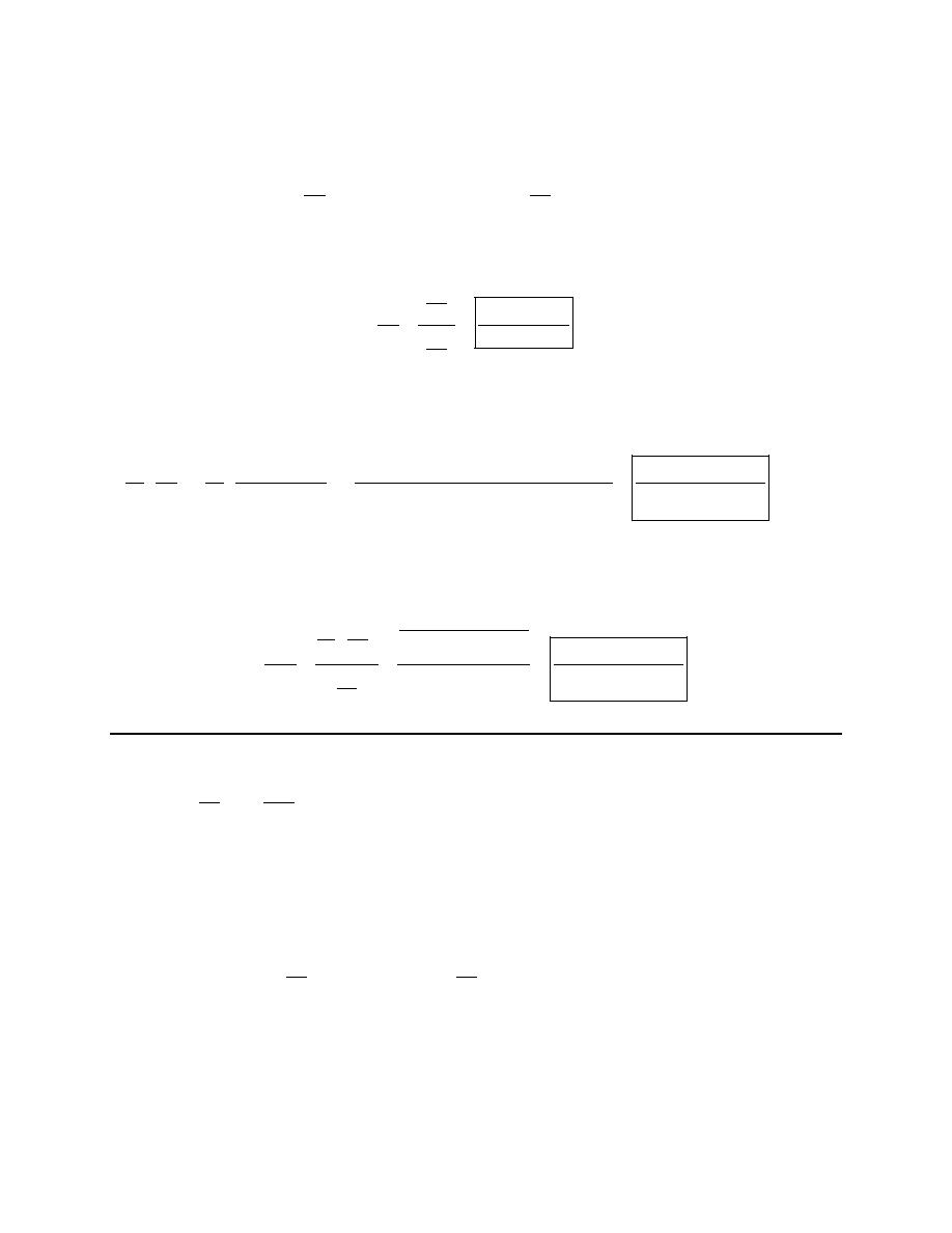
Calculus II

http://tutorial.math.lamar.edu/terms.aspx

Step 1
The first thing we’ll need here are the following two derivatives.

− +

Step 2
The first derivative is then,

− +

Step 3
For the second derivative we’ll now need,

( )(

)

(

)

(

)

(

)

dt dx

− + −

−





−



 =









− +









− +

Step 4
The second derivative is then,

(

)

(

)

d y

dt dx

−









− +

−





− +

2. Compute

and

d y

for the following set of parametric equations.

−

Step 1
The first thing we’ll need here are the following two derivatives.

−

= −

−

Step 2
The first derivative is then,

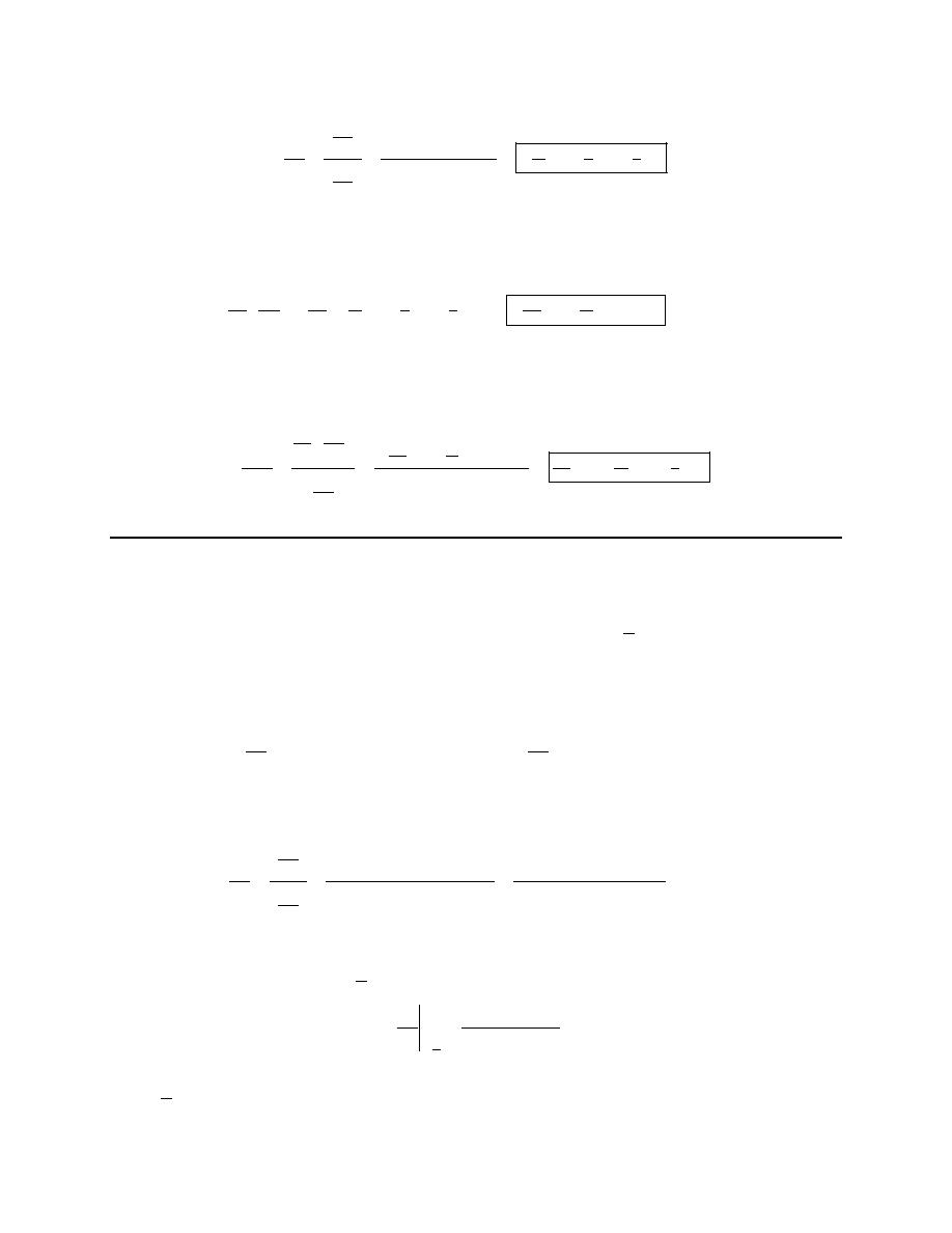
Calculus II

http://tutorial.math.lamar.edu/terms.aspx

−

= −

−

Step 3
For the second derivative we’ll now need,

(

)

108

dt dx



 = −

= −









Step 4
The second derivative is then,

108

d y

dt dx

−







 −





−

3. Find the equation of the tangent line(s) to the following set of parametric equations at the given point.

( )

2 cos 3

4 sin 3

3 tan 6

−

Step 1
We’ll need the first derivative for the set of parametric equations. We’ll need the following derivatives,

( )

6 sin 3

12 cos 3

18sec

= −

−

The first derivative is then,

( )

18sec

3sec

6 sin 3

12 cos 3

sin 3

2 cos 3

−

Step 2
The slope of the tangent line at

is then,

( )

( ) ( )

2 0

−

− − −

the parametric curve is at the point,

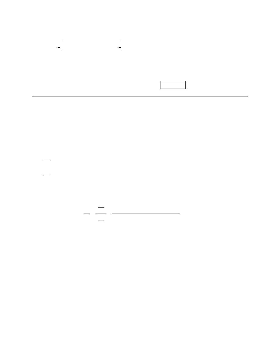
Calculus II

http://tutorial.math.lamar.edu/terms.aspx

( ) ( )

( )

2 0

3 0

4, 0

− − =

⇒

Step 3
The (only) tangent line for this problem is then,

(

)

0 3

= +

−

→

−

4. Find the equation of the tangent line(s) to the following set of parametric equations at the given point.

(

)

(

)

t t

= − −

−

(

)

3, 7

−

Step 1
We’ll need the first derivative for the set of parametric equations. We’ll need the following derivatives,

(

)

(

)

(

)

(

) (

)

(

)

(

)

t t

−

= −

−

= −

−

The first derivative is then,

(

)

(

)

(

)

t t

−

Hint : Don’t forget that because the derivative we found above is in terms of t we need to determine the
value(s) of t that put the parametric curve at the given point.
Step 2
Okay, the derivative we found above is in terms of t and we we’ll need to next determine the value(s) of t

that put the parametric curve at

(

)

3, 7

−

This is easy enough to do by setting the x and y coordinates equal to the known parametric equations and
determining the value(s) of t that satisfy both equations.

Doing that gives,

(

)(

)

− = − −

= − −
= −

→

= −

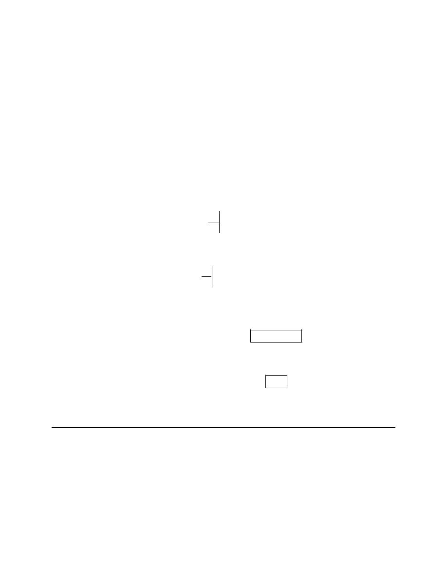
Calculus II

http://tutorial.math.lamar.edu/terms.aspx

(

)

(

)

(

) (

)

(

)

(

)

[

]

t t

−





= −

− −









= −

− −





= −

−

→

= −

We can see from this list that the parametric curve will be at

(

)

3, 7

−

for

= −

and

Step 3
From the previous step we can see that we will in fact have two tangent lines at the point. Here are the
slopes for each tangent line.

The slope of the tangent line at

= −

is,

=−

= −

and the slope of the tangent line at

is,

Step 4
The tangent line for

= −

is then,

(

)

7 24

= −

→

= −

−

The tangent line for

is then,

( )(

)

= −

→

Do not get excited about the second tangent line! It is just saying that the second tangent line is a
horizontal line.

5. Find the values of t that will have horizontal or vertical tangent lines for the following set of parametric
equations.

( )

2 cos 3

= −

−

Step 1
We’ll need the following derivatives for this problem.

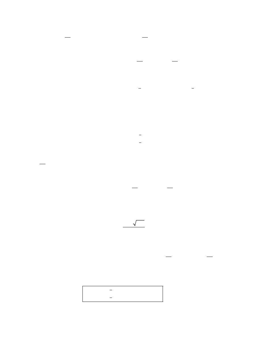
Calculus II

http://tutorial.math.lamar.edu/terms.aspx

( )

6 sin 3

−

= −

Step 2

We know that horizontal tangent lines will occur where

, provided

≠

at the same value of t.

So, to find the horizontal tangent lines we’ll need to solve,

( )

6 sin 3

sin 3

sin

0.7297

−

+ =

→

Also, a quick glance at a unit circle we can see that a second angle is,

0.7297

2.4119

= −

All possible values of t that will give horizontal tangent lines are then,

2
3

0.2432

0.7297

0, 1, 2, 3,

0.8040

2.4119 2

→

= ± ± ±



Note that we don’t officially know these do in fact give horizontal tangent lines until we also determine

that

≠

at these points. We’ll be able to determine that after the next step.

Step 3

We know that vertical tangent lines will occur where

, provided

≠

at the same value of t.

So, to find the vertical tangent lines we’ll need to solve,

(

)

964

0.3048,

5.9048

−

− =

→

= −

Step 4
From a quick inspection of the two lists of t values from Step 2 and Step 3 we can see there are no values

in common between the two lists. Therefore, any values of t that gives

will not give

and

visa-versa.

Therefore the values of t that gives horizontal tangent lines are,

2
3

0.2432

0, 1, 2, 3,

0.8040

π
π

= ± ± ±



Calculus II

http://tutorial.math.lamar.edu/terms.aspx

The values of t that gives vertical tangent lines are,

0.3048,

5.9048

= −

Area with Parametric Equations

1. Determine the area of the region below the parametric curve given by the following set of parametric
equations. You may assume that the curve traces out exactly once from right to left for the given range of
t. You should only use the given parametric equations to determine the answer.

−

= +

≤ ≤

Solution

There really isn’t too much to this problem. Just recall that the formula from the notes assumes that

( )

f t

and

( )

g t

. So, the area under the curve is,

(

)(

)

(

)

481568

105

4586.3619

t dt

−

∫
∫

2. Determine the area of the region below the parametric curve given by the following set of parametric
equations. You may assume that the curve traces out exactly once from right to left for the given range of
t. You should only use the given parametric equations to determine the answer.

( )

3 cos

4 sin

= −

= +

≤ ≤

Solution

There really isn’t too much to this problem. Just recall that the formula from the notes assumes that

( )

f t

and

( )

g t

. So, the area under the curve is,

Calculus II

http://tutorial.math.lamar.edu/terms.aspx

( )

(

)

( ) ( )

(

)

( ) ( )

( )

( ) ( )

( )

( ) ( )

( )

( ) ( )

( )

(

)

( )

(

)

1
2

3
4

3
8

4 sin

3cos

sin

12 cos

sin

3cos

sin

12 cos

sin

sin 2

12 cos

sin

12 cos

sin

1 cos 4

4 cos

sin 4

t dt

+ 







−

= −

−

= +

∫
∫

∫

You did recall how to do all the trig manipulations and trig integrals to do this integral correct? If not you
should go back to the

Integrals Involving Trig Functions

section to do some review/problems.

Arc Length with Parametric Equations

1. Determine the length of the parametric curve given by the following set of parametric equations. You
may assume that the curve traces out exactly once for the given range of t’s.

(

)

= + −

≤ ≤

Step 1
The first thing we’ll need here are the following two derivatives.

(

)

3
2

= −

−

Step 2
We’ll need the ds for this problem.

(

)

(

)

567

144

t dt









+ −

−













Step 3
The integral for the arc length is then,

567

∫

Step 4
This is a simple integral to compute with a quick substitution. Here is the integral work,

Calculus II

http://tutorial.math.lamar.edu/terms.aspx

( )(

)

(

)

567

1701

585

66.1865

−

∫

2. Determine the length of the parametric curve given by the following set of parametric equations. You
may assume that the curve traces out exactly once for the given range of t’s.

= +

= −

− ≤ ≤

Step 1
The first thing we’ll need here are the following two derivatives.

= −

Step 2
We’ll need the ds for this problem.

[ ] [ ]

t dt

+ −

Step 3
The integral for the arc length is then,

9 4

t dt

−

∫

Step 4
This integral will require a trig substitution (as will quite a few arc length integrals!).

Here is the trig substitution we’ll need for this integral.

tan

sec

θ θ

9 4

9 9 tan

3 1 tan

3 sec

To get rid of the absolute value on the secant will need to convert the limits into

limits.

( )

3
2

2 :

tan

0.9273

0 :

tan

−

= −

− =

→

= −

→

− = −

→

Okay, the corresponding range of

for this problem is

0.9273

−

≤ ≤

(fourth quadrant) and in this

range we know that secant is positive. Therefore the root becomes,

9 4

3sec

Calculus II

http://tutorial.math.lamar.edu/terms.aspx

The integral is then,

(

)

(

)

3
2

0.9273

9 4

3sec

sec

sec tan

ln sec

tan

7.4719

t dt

θ θ

−

= 







∫

3. A particle travels along a path defined by the following set of parametric equations. Determine the
total distance the particle travels and compare this to the length of the parametric curve itself.

( )

4 sin

1 2 cos

= −

−

≤ ≤

Hint : Be very careful with this problem. Note the two quantities we are being asked to find, how they
relate to each other and which of the two that we know how to compute from the material in this section.

Step 1
This is a problem that many students have issues with. First note that we are being asked to find both the
total distance traveled by the particle AND the length of the curve. Also, recall that of these two
quantities we only discussed how to determine the length of a curve in this section.

Therefore, let’s concentrate on finding the length of the curve first, then we’ll worry about the total
distance traveled.

Step 2
To find the length we’ll need the following two derivatives,

( )

( ) ( )

cos

sin

The ds for this problem is then,

( )

( ) ( )

( )

cos

sin

cos

sin

t dt

















Now, this is where many students run into issues with this problem. Many students use the following
integral to determine the length of the curve.

( )

cos

sin

t dt

−

∫

Can you see what is wrong with this integral?

Step 3
Remember from the discussion in this section that in order to use the arc length formula the curve can
only trace out exactly once over the range of the limits in the integral.

Calculus II

http://tutorial.math.lamar.edu/terms.aspx

Therefore, we can’t even write down the formula that we did in the previous step until we first determine
if the curve traces out exactly once in the given range of t’s.

If it turns out that the curve traces out more than once in the given range of t’s then the integral we wrote
down in the previous step is simply wrong. We will then need to determine a range of t’s for one trace so
we can write down the proper integral for the length.

Luckily enough for us we actually did this in a practice problem in the

Parametric Equations and Curves

section. Examining this set of parametric equations was problem #8 from that section. From the solution
to that problem we found a couple of pieces of information that will be needed for this problem.

First, we determined that the curve does trace out more than once in the given range of t’s for the
problem. In fact, we determined that the curve traced out 21.5 times over the given range of t’s.

Secondly, and more importantly at this point, we also determined that the curve would trace out exactly
once in the range of

−

≤ ≤

. Note that we actually listed several possible ranges of t’s for one

trace and we can use any of them. This is simply the first one found and so it’s the one we decided to use
for this problem.

So, we can now see that the integral we wrote down in the previous step was in fact not correct and will
not give the length of the curve.

Using the range of t’s we found in the earlier problem we can see that the integral for the length is,

( )

cos

sin

t dt

−

∫

Before proceeding with the next step we should address the fact that, in this case, we already had the
information in hand to write down the proper integral for the length. In most cases this will not be the
case and you will need to go back and do a shortened version of the analysis we did in the Parametric
Equations and Curves section. We don’t need all the information but to get the pertinent information we
will need to go through most of the analysis.

If you need a refresher on how to do that analysis you should go back to that section and work through a
few of the practice problems.

Step 4
Okay, let’s get to work on evaluating the integral. At first glance this looks like a really unpleasant
integral (and there’s no ignoring the fact that it’s not a super easy integral) however if we’re careful it
isn’t as difficult as it might appear at first glance.

First, let’s notice that we can do a little simplification as follows,

( )

(

)

( )

cos

1 sin

cos

1 sin

t dt

−

∫

As always, be very careful with the absolute value bars! Depending on the range of t’s we used for the
integral it might not be possible to just drop them. So, the next thing let’s do is determine how to deal
with them.

Calculus II

http://tutorial.math.lamar.edu/terms.aspx

We know that, for this integral, we used the following range of t’s.

−

≤ ≤

Now, notice that we don’t just have a t in the argument for the trig functions in our integral. In fact what
we have is

1
4

. So, we can see that as t ranges over

−

≤ ≤

we will get the following range for

1
4

(just divide the above inequality by 4!),

− ≤

≤

We know from our trig knowledge that as long as

1
4

stays in this range, which it will for our integral,

then

( )

1
4

cos

≥

and so we can drop the absolute values from the cosine in the integral.

As a final word of warning here keep in mind that for other ranges of t’s we might have had negative
cosine in the range of t’s and so we’d need to add in a minus sign to the integrand when we dropped the
absolute value bars. Whether or not we need to do this will depend upon the range of t’s we chose to use
for one trace and so this quick analysis will need to be done for these kinds of integrals.

Step 5
Okay, at this point the integral for the length of the curve is now,

( )

cos

1 sin

t dt

−

∫

This still looks to be an unpleasant integral. However, in this case note that we can use the following
simply substitution to convert it into a relatively easy integral.

( )

sin

cos

t dt

→

(

)

( )

2 :

sin

2 :

sin

= −

−

= −

Under this substitution the integral of the length of the curve is then,

4 1

u du

−

∫

Step 6
Now, at this point we can see that we have a fairly simple trig substitution we’ll need to evaluate to find
the length of the curve. The trig substitution we’ll need for this integral is,

tan

sec

1 tan

sec

θ θ

To get rid of the absolute value on the secant will need to convert the limits into

limits.

tan

= −

− =

→

= −

→

= −

→

Calculus II

http://tutorial.math.lamar.edu/terms.aspx

Okay, the corresponding range of

for this problem is

− ≤ ≤

(first and fourth quadrant) and in this

range we know that secant is positive. Therefore the root becomes,

sec

The length of the curve is then,

( )

(

)

cos

1 sin

4 1

4 sec

2 sec tan

ln sec

tan

9.1824

u du

θ θ

−

= 







∫

Step 7
Okay, that was quite a bit of work to get the length of the curve. We now need to recall that we were also
asked to get the total distance traveled by the particle. This is actually quite easy to get now that we have
the length of the curve.

To get the total distance traveled all we need to recall is that we noted in Step 3 above that we determined
in problem #8 from the

Parametric Equations and Curves

section that the curve will trace out 21.5 times.

Since we also know the length of a single trace of the curve we know that the total distance traveled by
the particle must be,

(

)(

)

Total Distance Travled

9.1824 21.5

197.4216

4. Set up, but do not evaluate, an integral that gives the length of the parametric curve given by the
following set of parametric equations. You may assume that the curve traces out exactly once for the
given range of t’s.

( )

sin 2

= +

≤ ≤

Step 1
The first thing we’ll need here are the following two derivatives.

( )

sin 2

2 cos 2

Step 2
We’ll need the ds for this problem.

[ ]

( )

sin 2

2 cos 2

sin 2

2 cos 2

















Step 3
The integral for the arc length is then,

Calculus II

http://tutorial.math.lamar.edu/terms.aspx

( )

sin 2

2 cos 2









⌠



⌡

∫

5. Set up, but do not evaluate, an integral that gives the length of the parametric curve given by the
following set of parametric equations. You may assume that the curve traces out exactly once for the
given range of t’s.

( )

(

)

3
2

cos 2

sin 1

−

− ≤ ≤

Step 1
The first thing we’ll need here are the following two derivatives.

( ) ( )

(

)

6 cos

2 sin 2

2 cos 1

= −

−

Step 2
We’ll need the ds for this problem.

( ) ( )

(

)

( )

(

)

6 cos

2 sin 2

2 cos 1

36 cos

2 sin

4 cos 1









−

+ −

−









−

Step 3
The integral for the arc length is then,

( )

(

)

36 cos

2 sin

4 cos 1

−

∫

Surface Area with Parametric Equations

1. Determine the surface area of the object obtained by rotating the parametric curve about the given axis.
You may assume that the curve traces out exactly once for the given range of t’s.

Rotate

3 2

9 3

= +

= −

≤ ≤

about the y-axis.

Step 1
The first thing we’ll need here are the following two derivatives.

Calculus II

http://tutorial.math.lamar.edu/terms.aspx

= −

Step 2
We’ll need the ds for this problem.

[ ] [ ]

+ −

Step 3
The integral for the surface area is then,

(

)

3 2

x ds

t dt

∫

Remember to be careful with the formula for the surface area! The formula used is dependent upon the
axis we are rotating about.

Step 4
This is a really simple integral…

(

)

3 2

13 3

t dt

∫

2. Determine the surface area of the object obtained by rotating the parametric curve about the given axis.
You may assume that the curve traces out exactly once for the given range of t’s.

Rotate

9 2

= +

≤ ≤ about the x-axis.

Step 1
The first thing we’ll need here are the following two derivatives.

Step 2
We’ll need the ds for this problem.

[ ] [ ]

Note that we factored a 16 out of the root to make the rest of the work a little simpler to deal with.

Step 3
The integral for the surface area is then,

Calculus II

http://tutorial.math.lamar.edu/terms.aspx

( )

(

)

y ds

t t

⌠

⌡

∫

Remember to be careful with the formula for the surface area! The formula used is dependent upon the
axis we are rotating about.

Step 4
This is a simple integral to compute with a quick substitution. Here is the integral work,

(

)

( )

341.1464

t t

− =

∫

3. Determine the surface area of the object obtained by rotating the parametric curve about the given axis.
You may assume that the curve traces out exactly once for the given range of t’s.

Rotate

( )

1
2

3cos

= +

≤ ≤ about the y-axis.

Step 1
The first thing we’ll need here are the following two derivatives.

( )

3 sin

= −

Step 2
We’ll need the ds for this problem.

( )

[ ]

( )

3 sin

sin

−









Step 3
The integral for the surface area is then,

( )

(

)

( )

1
2

3cos

sin

cos

sin

x ds

∫

Remember to be careful with the formula for the surface area! The formula used is dependent upon the
axis we are rotating about.

Step 4
Okay, this is a particularly unpleasant looking integral but we need to be able to deal with these kinds of
integrals on occasion. We’ll be able to do quite a bit of simplification if we first use the following
substitution.

( )

sin

cos

→

Calculus II

http://tutorial.math.lamar.edu/terms.aspx

( )

0 :

sin 0

sin

With this substitution the integral becomes,

∫

Step 5
This integral can be evaluated with the following (somewhat messy…) trig substitution.

tan

sec

θ θ

25 tan

5 tan

5 sec

+ =

To get rid of the absolute value on the secant will need to convert the limits into

limits.

( )

0 :

tan

1.0830

−

→

Okay, the corresponding range of

for this problem is

1.0830

≤ ≤

(first quadrant) and in this range

we know that secant is positive. Therefore the root becomes,

5sec

The surface area is then,

( )

(

)

( )

(

)

(

)

(

)

1.0830

3cos

sin

5sec

sec

sec tan

ln sec

tan

43.0705

∫

∫
∫
∫

This problem was a little messy but don’t let that make you decide that you can’t do these types of
problems! They can be done and often can be simplified with some relatively simple substitutions.

4. Set up, but do not evaluate, an integral that gives the surface area of the object obtained by rotating the
parametric curve about the given axis. You may assume that the curve traces out exactly once for the
given range of t’s.

Calculus II

http://tutorial.math.lamar.edu/terms.aspx

Rotate

(

)

1 ln 5

= +

−

≤ ≤

about the x-axis.

Step 1
The first thing we’ll need here are the following two derivatives.

2 4

= −

Step 2
We’ll need the ds for this problem.

[

]

(

)

(

)

2 4





+ −

−









Step 3
The integral for the surface area is then,

(

)

(

)

(

)

2 4

y ds

−

+ −

⌠



⌡

∫

Remember to be careful with the formula for the surface area! The formula used is dependent upon the
axis we are rotating about.

5. Set up, but do not evaluate, an integral that gives the surface area of the object obtained by rotating the
parametric curve about the given axis. You may assume that the curve traces out exactly once for the
given range of t’s.

Rotate

( )

1 3

sin 2 cos

= +

≤ ≤ about the y-axis.

Step 1
The first thing we’ll need here are the following two derivatives.

( )

2 cos 2 cos

sin 2 sin

−

Step 2
We’ll need the ds for this problem.

[ ]

( )

2 cos 2 cos

sin 2 sin





−





Step 3

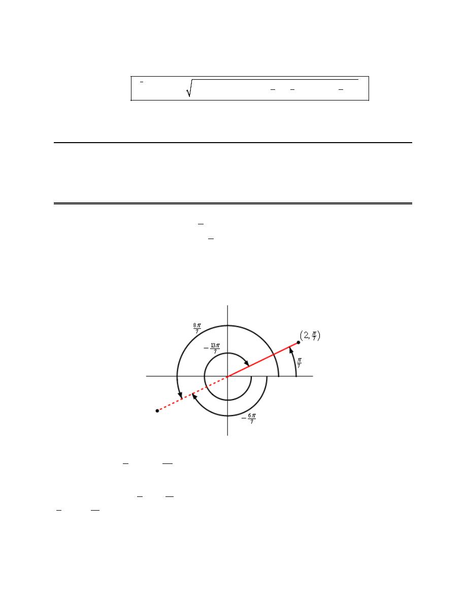
Calculus II

http://tutorial.math.lamar.edu/terms.aspx

The integral for the surface area is then,

(

)

( )

(

)

1 3

2 cos 2 cos

sin 2 sin

x ds

−

⌠

⌡

∫

Remember to be careful with the formula for the surface area! The formula used is dependent upon the
axis we are rotating about.

Polar Coordinates

1. For the point with polar coordinates

( )

determine three different sets of coordinates for the same

point all of which have angles different from

and are in the range

π θ

−

≤ ≤

Step 1
This problem is really as exercise in how well we understand the unit circle. Here is a quick sketch of the
point and some angles.

We can see that the negative angle ending at the solid red line that is in the range specified in the problem
statement is simply

−

= −

If we extend the solid line into the third quadrant (i.e. the dashed red line) then the positive angle ending
at the dashed red line is

+ =

. Likewise, the negative angle ending at the dashed red line is

− = −

With these angles getting the other three points should be pretty simple.

Calculus II

http://tutorial.math.lamar.edu/terms.aspx

Step 2
For the first “new” point we can use the negative angle that ends on the solid red line to get the point.

(

)

−

Step 3
For the remaining points recall that if we use a negative r then we go “backwards” from where the angle
ends to get the point. So, if we use

= −

, any angle that ends on the dashed red line will go

“backwards” into the first quadrant 2 units to get to the point.

This gives the remaining two points using both the positive and negative angle ending on the dashed red
line,

(

)

(

)

− −

−

2. The polar coordinates of a point are

(

)

5, 0.23

−

. Determine the Cartesian coordinates for the point.

Solution
There really isn’t too much to this problem. From the point we can see that we have

= −

and

0.23

(in radians of course!). Once we have these all we need to is plug into the formulas from this

section to get,

( ) (

)

( ) (

)

cos

5 cos 0.23

4.8683

sin

5 sin 0.23

1.1399

= −

So, the Cartesian coordinates for the point are then,

(

)

4.8683, 1.1399

−

3. The Cartesian coordinate of a point are

(

)

2, 6

−

. Determine a set of polar coordinates for the point.

Step 1
Let’s first determine r. That’s always simple.

( ) ( )

2 10

+ −

Step 2
Next let’s get

. As we do this we need to remember that we actually have two possible values of which

only one will work with the r we found in the first step.

Here are the two possible values of

Calculus II

http://tutorial.math.lamar.edu/terms.aspx

( )

tan

1.2490

1.8926

y
x

θ π

−

= −

+ =

So, we can see that

1.57

1.2490

− = −

= −

and so

is in the fourth quadrant. Likewise,

1.57

1.8926

3.14

< =

and so

is in the second quadrant.

We can also see from the Cartesian coordinates of the point that our point must be in the fourth quadrant
and so, for this problem,

is the correct value.

The polar coordinates of the point using the r from the first step and

from this step is,

(

)

2 10, 1.2490

−

Note of course that there are many other sets of polar coordinates that are just as valid for this
point. These are simply the set that we get from the formulas discussed in this section.

4. The Cartesian coordinate of a point are

(

)

8,1

−

. Determine a set of polar coordinates for the point.

Step 1
Let’s first determine r. That’s always simple.

( ) ( )

−

Step 2
Next let’s get

. As we do this we need to remember that we actually have two possible values of which

only one will work with the r we found in the first step.

Here are the two possible values of

( )

tan

0.1244

3.0172

y
x

θ π

−

= −

+ =

So, we can see that

1.57

0.1244

− = −

= −

and so

is in the fourth quadrant. Likewise,

1.57

3.0172

3.14

< =

and so

is in the second quadrant.

We can also see from the Cartesian coordinates of the point that our point must be in the second quadrant
and so, for this problem,

is the correct value.

The polar coordinates of the point using the r from the first step and

from this step is,

Calculus II

http://tutorial.math.lamar.edu/terms.aspx

(

)

65, 3.0172

Note of course that there are many other sets of polar coordinates that are just as valid for this
point. These are simply the set that we get from the formulas discussed in this section.

5. Convert the following equation into an equation in terms of polar coordinates.

= −

Solution
Basically what we need to do here is to convert all the x’s and y’s into r’s and

’s using the following

formulas.

cos

sin

Don’t forget about the last one! If it is possible to use this formula (and you can see where we’ll use it in
the case can’t you?) it will save a lot of work!

First let’s substitute in the equations as needed.

(

)

(

)(

)

cos

sin

= −

Finally, as we need to do is take care of little simplification to get,

4 cos

cos sin

= −

6. Convert the following equation into an equation in terms of polar coordinates.

−

Solution
Basically what we need to do here is to convert all the x’s and y’s into r’s and

’s using the following

formulas.

cos

sin

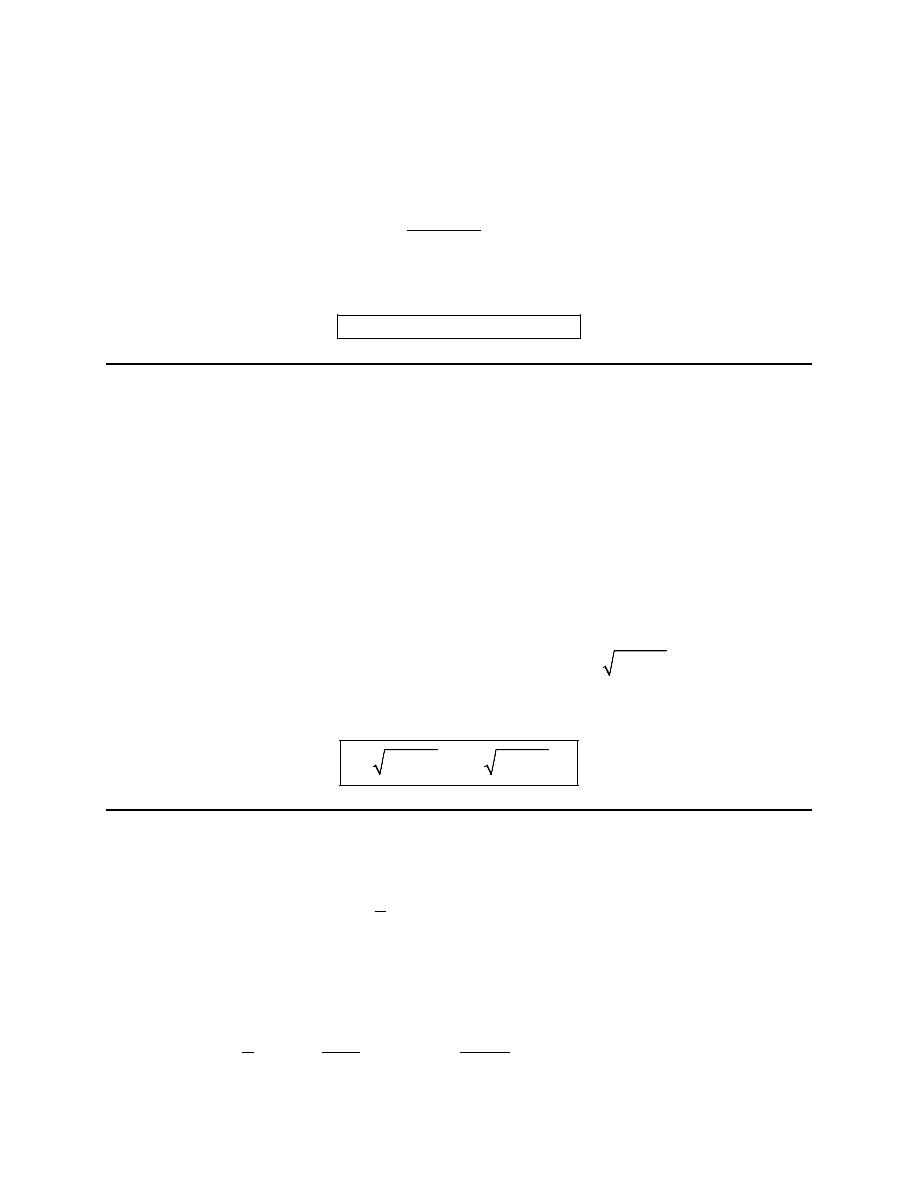
Calculus II

http://tutorial.math.lamar.edu/terms.aspx

Don’t forget about the last one! If it is possible to use this formula (which won’t do us a lot of good in
this problem) it will save a lot of work!

First let’s substitute in the equations as needed.

(

)

(

) (

)

cos

sin

−

Finally, as we need to do is take care of little simplification to get,

cos

4 cot

sin

−

7. Convert the following equation into an equation in terms of Cartesian coordinates.

sin

4 cos

= −

Solution
There is a variety of ways to work this problem. One way is to first multiply everything by r and then
doing a little rearranging as follows,

(

)

sin

cos

sin

cos

−

⇒

−

We can now use the following formulas to finish this problem.

cos

sin

Here is the answer for this problem,





−





8. Convert the following equation into an equation in terms of Cartesian coordinates.

sin

sec

−

Solution
There is a variety of ways to work this problem. One way is to first do the following
rearranging/rewriting of the equation.

2 cos

sin

sin cos

cos

−

→

−

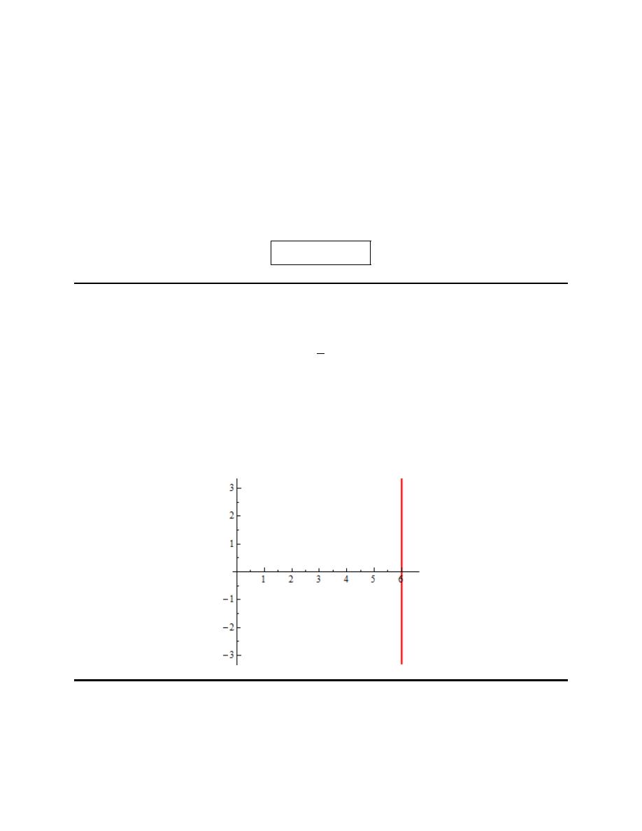
Calculus II

http://tutorial.math.lamar.edu/terms.aspx

At this point we can multiply everything by

and do a little rearranging as follows,

(

)(

)

2 cos

sin cos

2 cos

sin

cos

−

→

−

We can now use the following formulas to finish this problem.

cos

sin

Here is the answer for this problem,

(

)

−

9. Sketch the graph of the following polar equation.

cos

Solution
Multiplying both sides by r gives,

cos

and we know from the notes on this section that this is simply the vertical line

. So here is the graph

of this function.

10. Sketch the graph of the following polar equation.

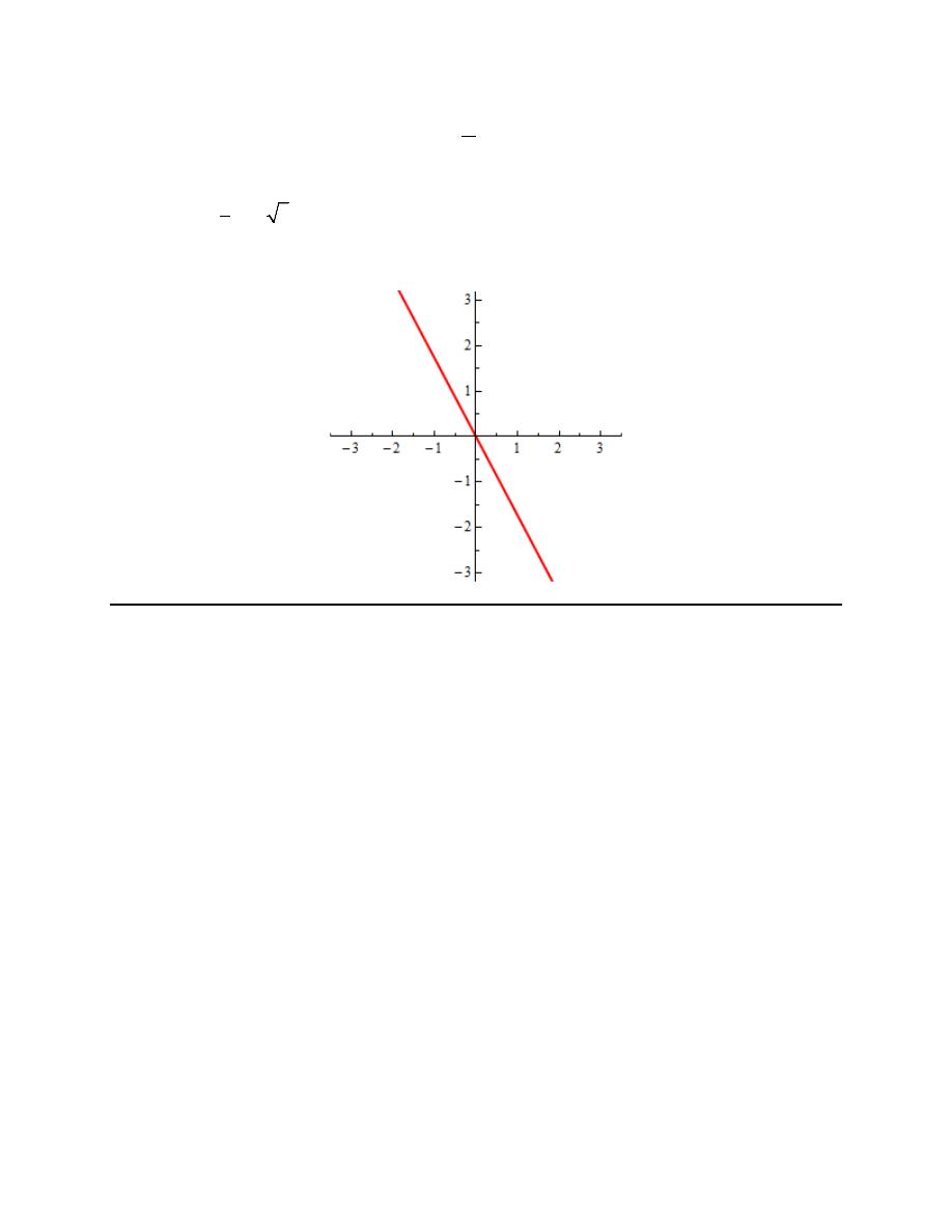
Calculus II

http://tutorial.math.lamar.edu/terms.aspx

= −

Solution
We know from the notes on this section that this is simply the line that goes through the origin and has

slope of

( )

tan

−

= −

So here is the graph of this function.

11. Sketch the graph of the following polar equation.

14 cos

= −

Solution
We can rewrite this as,

( )

7 cos

= −

and so we know from the notes on this section that this is simply the circle with radius -7 and center

(

)

7, 0

−

So here is the graph of this function.

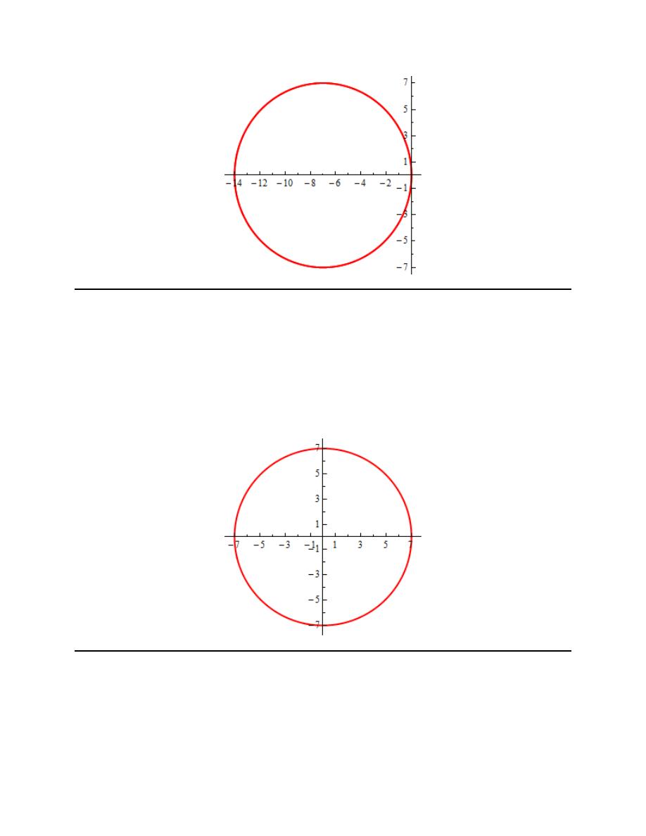
Calculus II

http://tutorial.math.lamar.edu/terms.aspx

12. Sketch the graph of the following polar equation.

Solution
We know from the notes on this section that this is simply the circle with radius 7 and centered at the
origin.

So here is the graph of this function.

13. Sketch the graph of the following polar equation.

9 sin

Solution
We can rewrite this as,

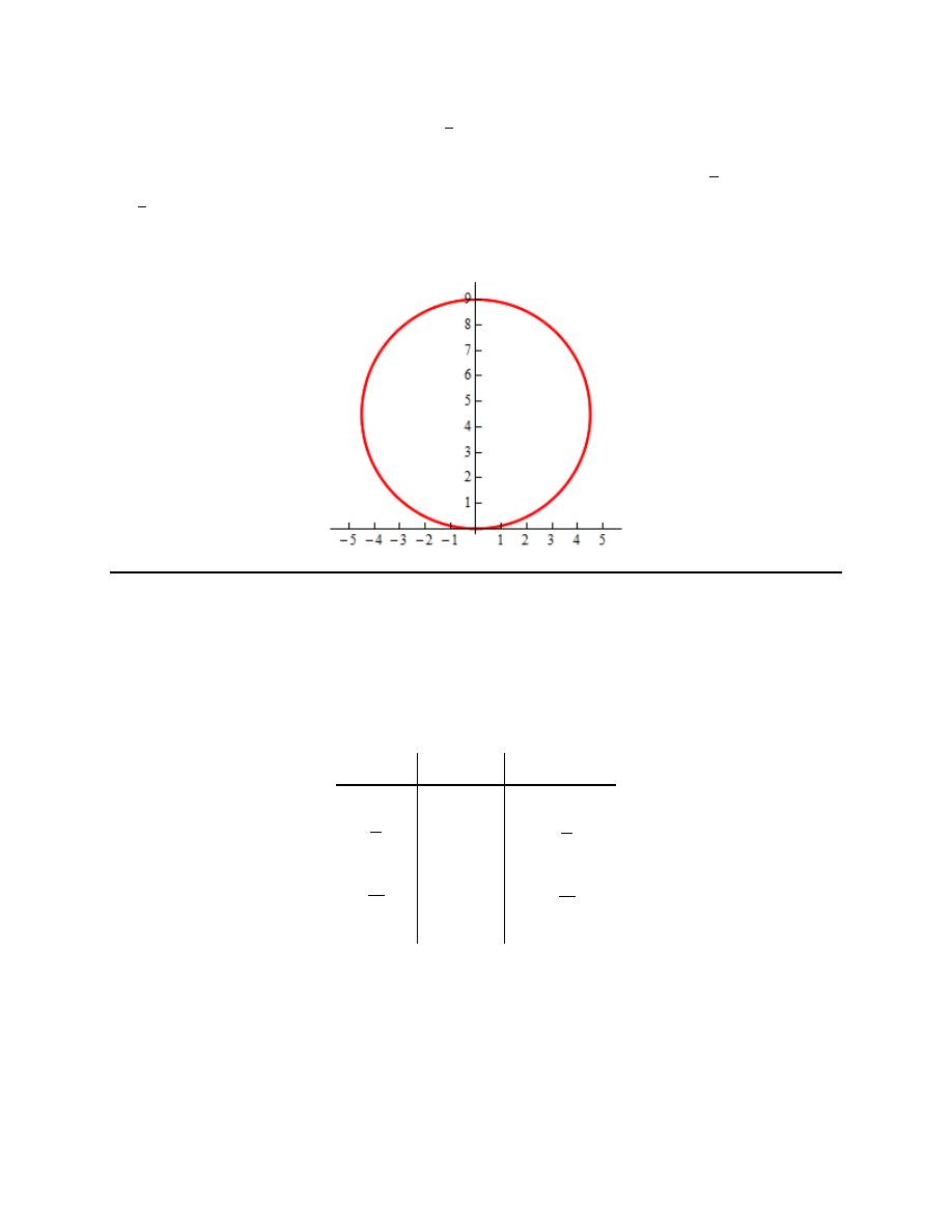
Calculus II

http://tutorial.math.lamar.edu/terms.aspx

( )

9
2

sin

and so we know from the notes on this section that this is simply the circle with radius

9
2

and center

( )

9
2

So here is the graph of this function.

14. Sketch the graph of the following polar equation.

8 8 cos

= +

Solution
We know from the notes on this section that this is a cardioid and so all we really need to get the graph is
a quick chart of points.

( )

(

)

16, 0

( )

(

)

(

)

16, 2

So here is the graph of this function.

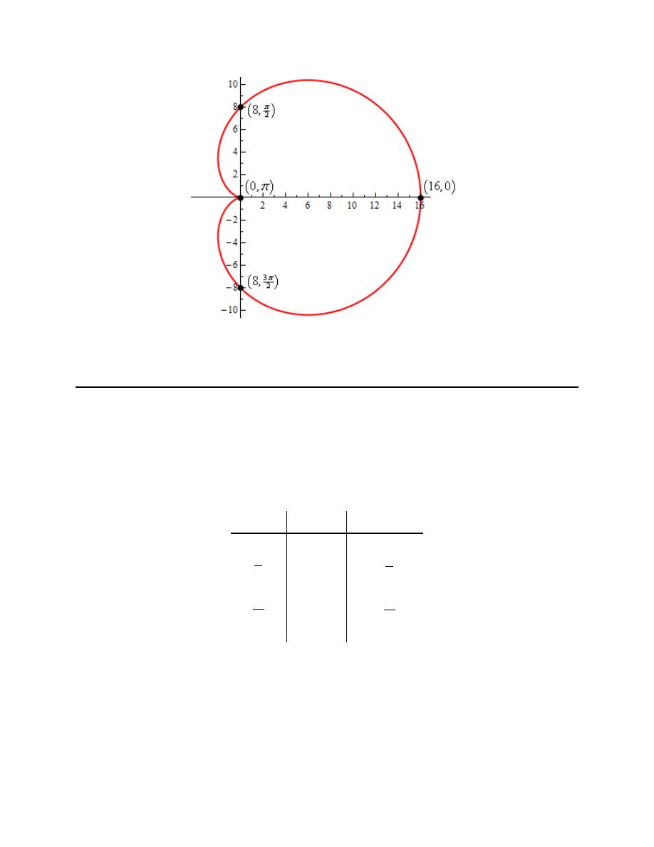
Calculus II

http://tutorial.math.lamar.edu/terms.aspx

15. Sketch the graph of the following polar equation.

5 2 sin

= −

Solution
We know from the notes on this section that this is a limacon without an inner loop and so all we really
need to get the graph is a quick chart of points.

( )

5, 0

( )

(

)

(

)

5, 2

So here is the graph of this function.

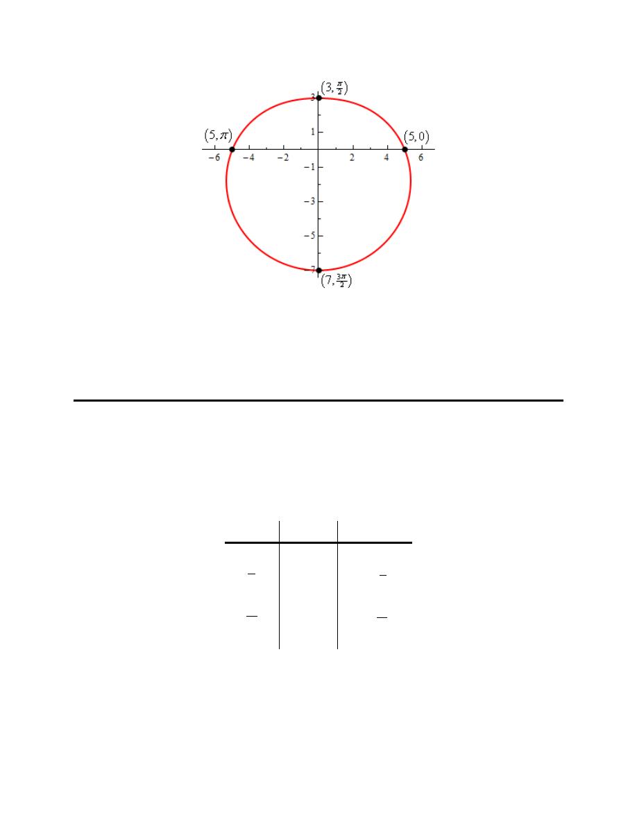
Calculus II

http://tutorial.math.lamar.edu/terms.aspx

Be careful when plotting these points and remember the rules for graphing polar coordinates. The “tick
marks” on the graph are really the Cartesian coordinate tick marks because those are the ones we are
familiar with. Do not let them confuse you when you go to plot the polar points for our sketch.

Also, many of these graphs are vaguely heart shaped although as this sketch has shown many do and this
one is more circular than heart shaped.

16. Sketch the graph of the following polar equation.

4 9 sin

= −

Solution
We know from the notes on this section that this is a limacon with an inner loop and so all we really need
to get the graph is a quick chart of points.

( )

4, 0

-5

(

)

−

( )

(

)

13,

(

)

4, 2

So here is the graph of this function.

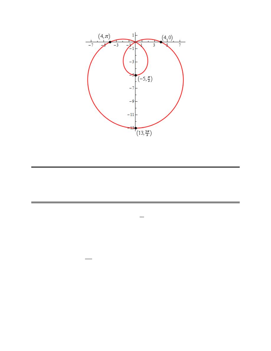
Calculus II

http://tutorial.math.lamar.edu/terms.aspx

Tangents with Polar Coordinates

1. Find the tangent line to

( ) ( )

sin 4

cos

Step 1
First, we’ll need to following derivative,

( ) ( )

4 cos 4

cos

sin 4

sin

−

Step 2
Next using the formula from the notes on this section we have,

Calculus II

http://tutorial.math.lamar.edu/terms.aspx

( ) ( )

(

)

( ) ( )

(

)

( ) ( )

(

)

( ) ( )

(

)

sin

cos

sin

4 cos 4

cos

sin 4

sin

sin 4

cos

4 cos 4

cos

sin 4

sin

cos

sin 4

cos

sin

−

This is a very messy derivative (these often are) and, at least in this case, there isn’t a lot of simplification
that we can do…

Step 3

Next we’ll need to evaluate both the derivative from the previous step as well as r at

3 3

You can see why we need both of these right?

Step 4

Lastly we need the x and y coordinate that we’ll be at when

. These values are easy enough to find

given that we know what r is at this point and we also know the polar to Cartesian coordinate conversion
formulas. So,

( )

3 3

cos

sin

Of course we also have the slope of the tangent line since it is just the value of the derivative we
computed in the previous step.

Step 5
The tangent line is then,

(

)

3 3

= +

−

2. Find the tangent line to

( )

cos

= −

Step 1
First, we’ll need to following derivative,

Calculus II

http://tutorial.math.lamar.edu/terms.aspx

( )

1 sin

= +

Step 2
Next using the formula from the notes on this section we have,

( )

(

)

( )

(

)

( )

(

)

( )

(

)

sin

cos

sin

1 sin

sin

cos

1 sin

cos

sin

−

This is a somewhat messy derivative (these often are) and, at least in this case, there isn’t a lot of
simplification that we can do…

Step 3

Next we’ll need to evaluate both the derivative from the previous step as well as r at

0.2843

3.0633

You can see why we need both of these right?

Step 4

Lastly we need the x and y coordinate that we’ll be at when

. These values are easy enough to

find given that we know what r is at this point and we also know the polar to Cartesian coordinate
conversion formulas. So,

( )

cos

3.0633cos

2.1661

sin

3.0633sin

2.1661

= −

Of course we also have the slope of the tangent line since it is just the value of the derivative we
computed in the previous step.

Step 5
The tangent line is then,

(

)

2.1661 0.2843

2.1661

0.2843

2.7819

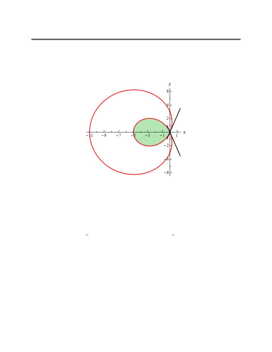
Calculus II

http://tutorial.math.lamar.edu/terms.aspx

Area with Polar Coordinates

1. Find the area inside the inner loop of

3 8 cos

= −

Step 1
First, here is a quick sketch of the graph of the region we are interested in.

Step 2
Now, we’ll need to determine the values of

that the graph goes through the origin (indicated by the

black lines on the graph in the previous step).

There are easy enough to find. Because they are where the graph goes through the origin we know that
we must have

. So,

( )

3 8 cos

cos

1.1864

θ
θ

−

=
=

⇒

This is the angle in the first quadrant where the graph goes through the origin.

We next need the angle in the fourth quadrant. We need to be a little careful with this second angle. We
need to always remember that the limits on the integral we’ll eventually be computing must go from
smaller to larger value. Also, as the angle moves from the smaller to larger value they must trace out the
boundary curve of the region we are interested in.

From a quick sketch of a unit circle we can quickly get two possible values for the angle in the fourth
quadrant.

1.1864

5.0968

1.1864

−

= −

Calculus II

http://tutorial.math.lamar.edu/terms.aspx

Depending upon the problem we are being asked to do either of these could be the one we need.
However, in this case we can see that if we use the first angle (i.e. the positive angle) we actually end up
tracing out the outer portion of the curve and that isn’t what we want here. However, if we use the second
angle (i.e. the negative angle) we will trace out the inner loop as we move from this angle to the angle in
the first quadrant.

So, for this particular problem, we need to use

1.1864

= −

The ranges of

for this problem is then

1.1864

−

≤ ≤

Step 3
The area of the inner loop is then,

(

)

( )

(

)

( )

(

)

1.1864

1
2

1.1864

1
2

1.1864

1
2

1.1864

1
2

1.1864

1
2

1.1864

3 8 cos

9 48 cos

64 cos

9 48 cos

32 1 cos 2

41 48 cos

32 cos 2

48sin

16 sin 2

15.2695

θ θ

−

∫

∫
∫
∫

Make sure you can do the trig manipulations required to do these integrals. Most of the
integrals in this section will involve this kind of manipulation. If you don’t recall how to do
them go back and take a look at the

Integrals Involving Trig Functions

section.

2. Find the area inside the graph of

7 3cos

= +

and to the left of the y-axis.

Step 1
First, here is a quick sketch of the graph of the region we are interested in.

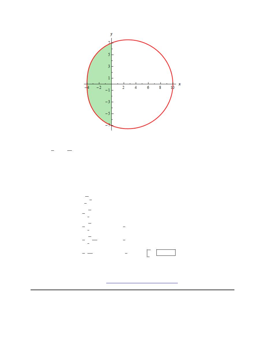
Calculus II

http://tutorial.math.lamar.edu/terms.aspx

Step 2
For this problem there isn’t too much difficulty in getting the limits for the problem. We will need to use
the limits

≤ ≤

to trace out the portion of the graph to the left of the y-axis.

Remember that it is important to trace out the portion of the curve defining the area we are interested in as
the

’s increase from the smaller to larger value.

Step 3
The area is then,

(

)

( )

(

)

( )

(

)

1
2

107

1
2

107

1
2

7 3cos

49 42 cos

9 cos

49 42 cos

1 cos 2

42 cos

cos 2

42 sin

sin 2

42.0376

θ θ

∫

∫
∫
∫

Integrals Involving Trig Functions

section.

3. Find the area that is inside

3 3sin

= +

and outside

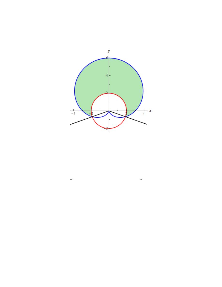
Calculus II

http://tutorial.math.lamar.edu/terms.aspx

Step 1
First, here is a quick sketch of the graph of the region we are interested in.

Step 2
Now, we’ll need to determine the values of

where the graphs intersect (indicated by the black lines on

the graph in the previous step).

There are easy enough to find. Because they are where the graphs intersect we know they must have the
same value of r. So,

( )

3 3sin

sin

0.3398

θ
θ

−

=
= −

⇒

− = −

This is the angle in the fourth quadrant where the graphs intersect.

From a quick sketch of a unit circle we can quickly get the angle in the third quadrant where the two
graphs intersect.

0.3398

3.4814

θ π

= +

The ranges of

for this problem is then

0.3398

3.4814

−

≤ ≤

Step 3
From the graph we can see that

3 3sin

= +

is the “outer” graph for this region and

is the

“inner” graph.

The area then,

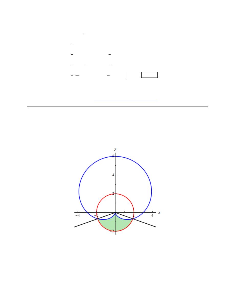
Calculus II

http://tutorial.math.lamar.edu/terms.aspx

(

) ( )

( )

(

)

( )

(

)

3.4814

1
2

0.3398

3.4814

1
2

0.3398

3.4814

1
2

0.3398

3.4814

1
2

0.3398

3.4814

1
2

0.3398

3 3sin

5 18sin

9 sin

5 18sin

1 cos 2

18sin

cos 2

18 cos

sin 2

33.7074

θ θ

−





−





−

∫

∫
∫
∫

Integrals Involving Trig Functions

section.

4. Find the area that is inside

3 3sin

= +

and outside

Step 1
First, here is a quick sketch of the graph of the region we are interested in.

Step 2
Now, we’ll need to determine the values of

where the graphs intersect (indicated by the black lines on

the graph in the previous step).

There are easy enough to find. Because they are where the graphs intersect we know they must have the
same value of r. So,

Calculus II

http://tutorial.math.lamar.edu/terms.aspx

( )

3 3sin

sin

0.3398

θ
θ

−

=
= −

⇒

− = −

This is one possible value for the angle in the fourth quadrant where the graphs intersect.

From a quick sketch of a unit circle we can quickly get the angle in the third quadrant where the two
graphs intersect.

0.3398

3.4814

θ π

= +

Now, we’ll have a problem if we use these two angles for our area integral. Recall that the angles must
go from smaller to larger values and as they do that they must trace out the boundary curves of the
enclosed area. These two clearly will not do that. In fact they trace out the area from the previous
problem.

To fix this problem it is probably easiest to use a quick sketch of a unit circle to see that another value for
the angle in the fourth quadrant is,

0.3398

5.9434

−

Using this angle along with the angle we already have in the third quadrant will trace out the area we are
interested in.

Therefore, the ranges of

for this problem is then

3.4814

5.9434

≤ ≤

Step 3
From the graph we can see that

is the “outer” graph for this region and

3 3sin

= +

is the

“inner” graph.

The area then,

( ) (

)

( )

(

)

( )

(

)

5.9434

1
2

3.4814

5.9434

1
2

3.4814

5.9434

1
2

3.4814

5.9434

1
2

3.4814

5.9434

1
2

3.4814

3 3sin

5 18sin

9 sin

5 18sin

1 cos 2

18sin

cos 2

18 cos

sin 2

3.8622

θ θ





− +





− −

−

− −

−

− −

= −

∫

∫
∫
∫

Do not get too excited about all the minus signs in the second step above. Just because all the
terms have minus signs in front of them does not mean that we should get a negative value from
out integral!

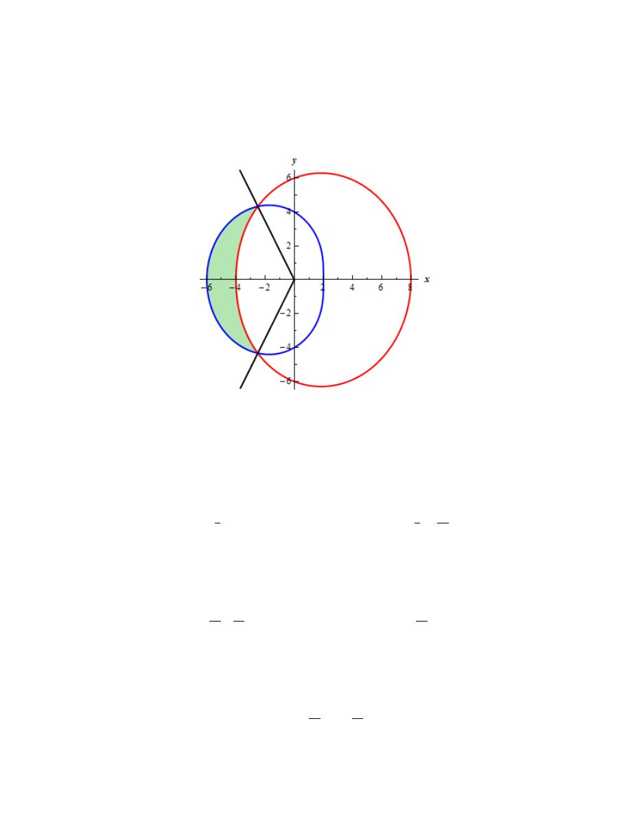
Calculus II

http://tutorial.math.lamar.edu/terms.aspx

5. Find the area that is inside

4 2 cos

= −

and outside

6 2 cos

= +

Step 1
First, here is a quick sketch of the graph of the region we are interested in.

Step 2
Now, we’ll need to determine the values of

where the graphs intersect (indicated by the black lines on

the graph in the previous step).

There are easy enough to find. Because they are where the graphs intersect we know they must have the
same value of r. So,

( )

6 2 cos

4 2 cos

cos

−

= −
= −

⇒

− =

This is the value for the angle in the second quadrant where the graphs intersect.

From a quick sketch of a unit circle we can quickly see two possible values for the angle in the third
quadrant where the two graphs intersect.

−

= −

Now, we need to recall that the angles must go from smaller to larger values and as they do that they must
trace out the boundary curves of the enclosed area. Keeping this in mind and we can see that we’ll need
to use the positive angle for this problem. If we used the negative angle we’d be tracing out the “right”
portions of our curves and we need to trace out the “left” portions of our curves.

Therefore, the ranges of

for this problem is then

≤ ≤

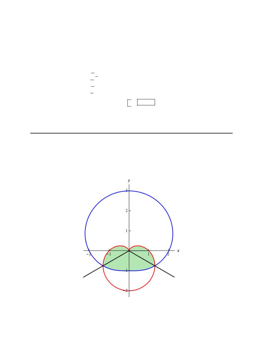
Calculus II

http://tutorial.math.lamar.edu/terms.aspx

Step 3
From the graph we can see that

4 2 cos

= −

is the “outer” graph for this region and

2 cos

= +

the “inner” graph.

The area then,

(

) (

)

( )

(

)

1
2

4 2 cos

6 2 cos

10 20 cos

20 sin

13.6971

θ θ





−

− +





− −

= −

−

∫
∫

Do not get too excited about all the minus signs in the integral. Just because all the terms have
minus signs in front of them does not mean that we should get a negative value from out integral!

6. Find the area that is inside both

1 sin

= −

and

2 sin

= +

Step 1
First, here is a quick sketch of the graph of the region we are interested in.

Step 2

Calculus II

http://tutorial.math.lamar.edu/terms.aspx

Now, we’ll need to determine the values of

where the graphs intersect (indicated by the black lines on

the graph in the previous step).

There are easy enough to find. Because they are where the graphs intersect we know they must have the
same value of r. So,

( )

2 sin

1 sin

sin

−

= −
= −

⇒

− = −

This is one possible value for the angle in the fourth quadrant where the graphs intersect. From a quick
sketch of a unit circle we can see that a second possible value for this angle is,

− =

From a quick sketch of a unit circle we can quickly get a value for the angle in the third quadrant where
the two graphs intersect.

θ π

= + =

Okay. We now have a real problem. Recall that the angles must go from smaller to larger values and as
they do that they must trace out the boundary curves of the enclosed area.

If we use

− ≤ ≤

we actually end up tracing out the large “open” or unshaded region that lies

above the shaded region.

Likewise, if we use

≤ ≤

we actually end up tracing out the smaller “open” or unshaded region

that lies below the shaded region.

In other words, we can’t find the shaded area simply by using the formula from this section.

Step 3
As we saw in the previous step we can’t just compute an integral in order to get the area of the shaded
region. However, that doesn’t mean that we can’t find the area of the shaded region. We just need to
work a little harder at it for this problem.

To find the area of the shaded area we can notice that the shaded area is really nothing more than the
remainder of the area inside

2 sin

= +

once we take out the portion that is also outside

1 sin

= −

Another way to look at is that the shaded area is simply the remainder of the area inside

1 sin

= −

once we take out the portion that is also outside

2 sin

= +

We can use either of these ideas to find the area of the shaded region. We’ll use the first one for no other
reason that it was the first one listed.

If we knew the total area that is inside

2 sin

= +

(which we can find with a simple integral) and if we

also knew the area that is inside

2 sin

= +

and outside

1 sin

= −

then the shaded area is nothing

more than the difference between these two areas.

Calculus II

http://tutorial.math.lamar.edu/terms.aspx

Step 4
Okay, let’s start this off by getting the total area that is inside

2 sin

= +

. This can be found by

evaluating the following integral.

(

)

( )

(

)

( )

(

)

1
2

2 sin

4 4 sin

sin

4 4 sin

1 cos 2

4 sin

cos 2

4 cos

sin 2

θ θ

−

∫

∫
∫
∫

Note that we need to do a full “revolution” to get all the area inside

2 sin

= +

and so we used the

range

≤ ≤

for this integral.

Step 5
Now, the area that is inside

2 sin

= +

and outside

1 sin

= −

is,

(

) (

)

( )

(

)

1
2

2 sin

1 sin

3 6 sin

6 cos

3 3

θ θ

−





− −





−

∫

Note that we found the limits for this region in Step 2.

Step 6

Finally the shaded area is simply,

(

)

3 3

2.6578

−

Arc Length with Polar Coordinates

1. Determine the length of the following polar curve. You may assume that the curve traces out exactly
once for the given range of

4 sin

= −

θ π

≤ ≤

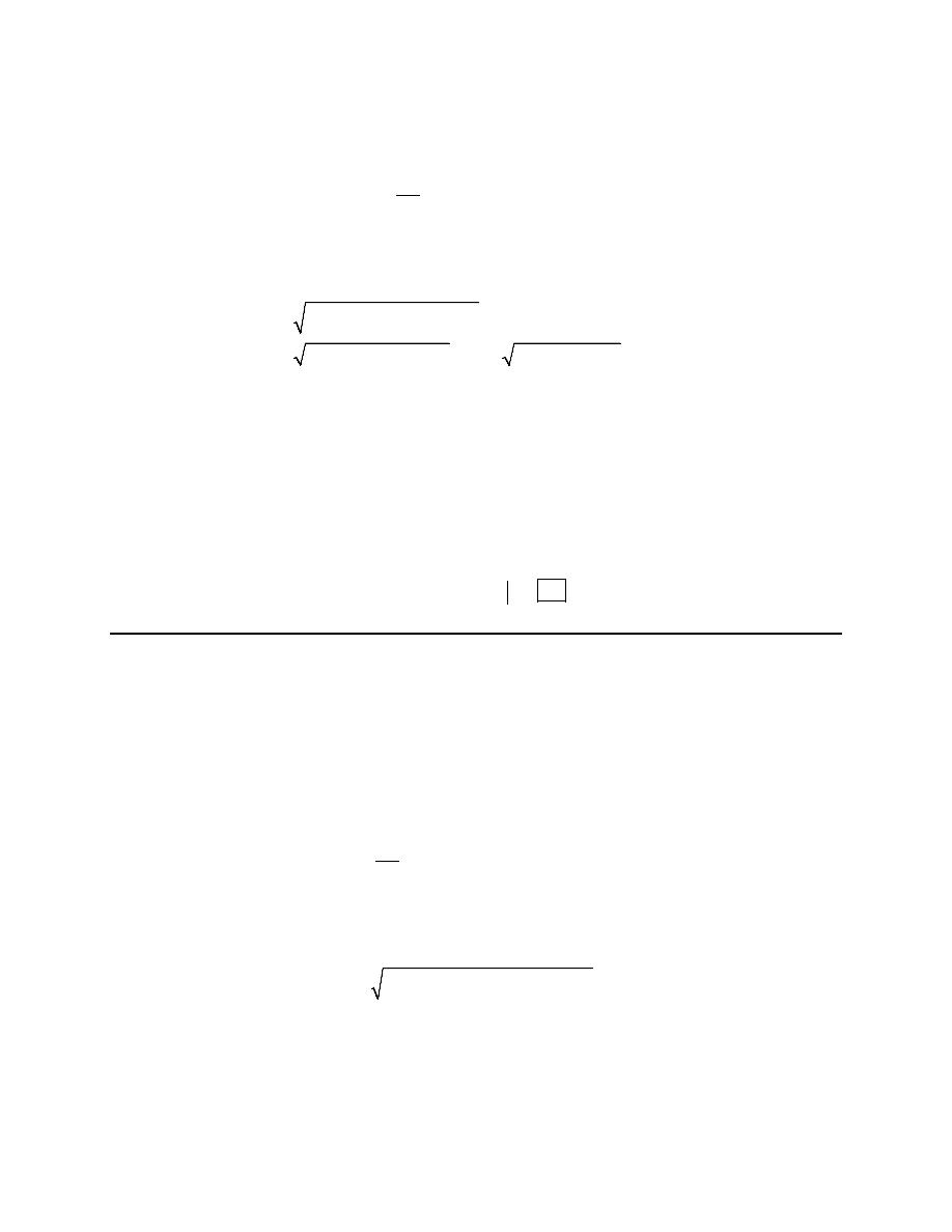
Calculus II

http://tutorial.math.lamar.edu/terms.aspx

Step 1
The first thing we’ll need here is the following derivative.

4 cos

= −

Step 2
We’ll need the ds for this problem.

[

] [

]

4 sin

4 cos

16 sin

16 cos

4 sin

cos

θ θ

−

+ −

Step 3
The integral for the arc length is then,

∫

Step 4
This is a really simple integral to compute. Here is the integral work,

∫

2. Set up, but do not evaluate, and integral that gives the length of the following polar curve. You may
assume that the curve traces out exactly once for the given range of

cos

θ π

≤ ≤

Step 1
The first thing we’ll need here is the following derivative.

cos

sin

θ θ

−

Step 2
We’ll need the ds for this problem.

[

] [

]

cos

sin

θ θ

−

Step 3
The integral for the arc length is then,

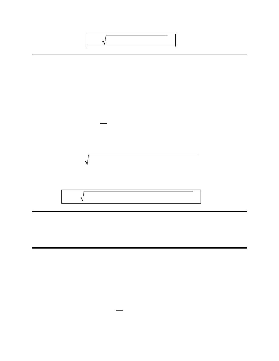
Calculus II

http://tutorial.math.lamar.edu/terms.aspx

[

] [

]

cos

sin

θ θ

−

∫

3. Set up, but do not evaluate, and integral that gives the length of the following polar curve. You may
assume that the curve traces out exactly once for the given range of

( )

cos 2

sin 3

≤ ≤

Step 1
The first thing we’ll need here is the following derivative.

( )

2 sin 2

3cos 3

= −

Step 2
We’ll need the ds for this problem.

( )

cos 2

sin 3

2 sin 2

3cos 3

+ −

















Step 3
The integral for the arc length is then,

( )

cos 2

sin 3

2 sin 2

3cos 3

+ −

















⌠

⌡

Surface Area with Polar Coordinates

1. Set up, but do not evaluate, an integral that gives the surface area of the curve rotated about the given
axis. You may assume that the curve traces out exactly once for the given range of

5 4 sin

= −

θ π

≤ ≤ rotated about the x-axis.

Step 1
The first thing we’ll need here is the following derivative.

4 cos

= −

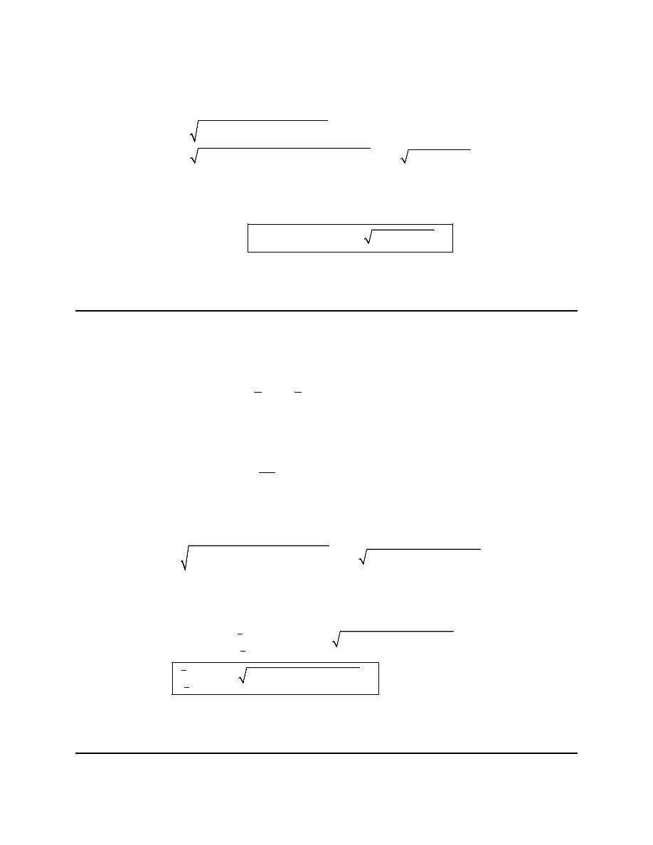
Calculus II

http://tutorial.math.lamar.edu/terms.aspx

Step 2
We’ll need the ds for this problem.

[

] [

]

5 4 sin

4 cos

25 40 sin

16 sin

16 cos

41 40 sin

θ θ

−

+ −

−

Step 3
The integral for the surface area is then,

(

)

5 4 sin

sin

41 40 sin

y ds

θ θ

−

∫

Remember to be careful with the formula for the surface area! The formula used is dependent upon the
axis we are rotating about. Also, do not forget to substitute the polar conversion formula for y!

2. Set up, but do not evaluate, an integral that gives the surface area of the curve rotated about the given
axis. You may assume that the curve traces out exactly once for the given range of

cos

− ≤ ≤ rotated about the y-axis.

Step 1
The first thing we’ll need here is the following derivative.

2 cos sin

= −

Step 2
We’ll need the ds for this problem.

[

]

cos

2 cos sin

cos

4 cos

sin

θ θ





+ −





Step 3
The integral for the surface area is then,

(

)

cos

4 cos

sin

2 cos

cos

4 cos

sin

x ds

θ θ

−

∫

Remember to be careful with the formula for the surface area! The formula used is dependent upon the
axis we are rotating about. Also, do not forget to substitute the polar conversion formula for x!

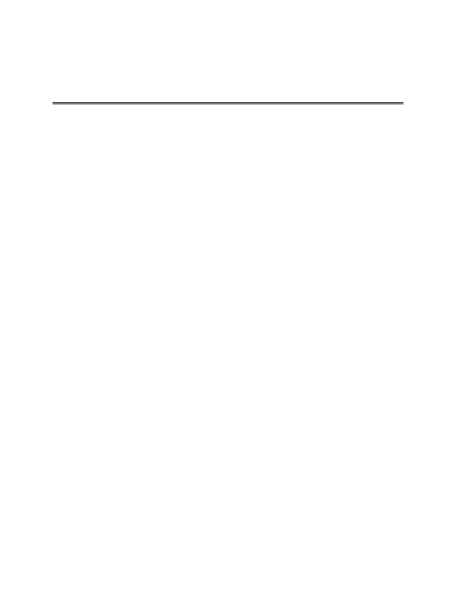
Calculus II

http://tutorial.math.lamar.edu/terms.aspx

Arc Length and Surface Area Revisited

Problems have not yet been written for this section and probably won’t be to be honest since this is just a
summary section.