CalcII_ParametricEqns_PolarCoords pdf - عبدالرحمن سهيل

CALCULUS II

Parametric Equations and Polar Coordinates

Paul Dawkins

Calculus II

http://tutorial.math.lamar.edu/terms.aspx

Table of Contents

Preface ............................................................................................................................................ ii

Parametric Equations and Polar Coordinates ............................................................................ 3

Introduction ................................................................................................................................................ 3

Parametric Equations and Curves .............................................................................................................. 5

Tangents with Parametric Equations .........................................................................................................25

Area with Parametric Equations ................................................................................................................32

Arc Length with Parametric Equations .....................................................................................................35

Surface Area with Parametric Equations...................................................................................................39

Polar Coordinates ......................................................................................................................................41

Tangents with Polar Coordinates ..............................................................................................................51

Area with Polar Coordinates .....................................................................................................................53

Arc Length with Polar Coordinates ...........................................................................................................60

Surface Area with Polar Coordinates ........................................................................................................62

Arc Length and Surface Area Revisited ....................................................................................................63

Calculus II

http://tutorial.math.lamar.edu/terms.aspx

Preface

Here are my online notes for my Calculus II course that I teach here at Lamar University.
Despite the fact that these are my “class notes”, they should be accessible to anyone wanting to
learn Calculus II or needing a refresher in some of the topics from the class.

These notes do assume that the reader has a good working knowledge of Calculus I topics
including limits, derivatives and basic integration and integration by substitution.

Calculus II tends to be a very difficult course for many students.  There are many reasons for this.

The first reason is that this course does require that you have a very good working knowledge of
Calculus I. The Calculus I portion of many of the problems tends to be skipped and left to the
student to verify or fill in the details. If you don’t have good Calculus I skills, and you are
constantly getting stuck on the Calculus I portion of the problem, you will find this course very
difficult to complete.

The second, and probably larger, reason many students have difficulty with Calculus II is that you
will be asked to truly think in this class.  That is not meant to insult anyone; it is simply an
acknowledgment that you can’t just memorize a bunch of formulas and expect to pass the course
as you can do in many math classes. There are formulas in this class that you will need to know,
but they tend to be fairly general. You will need to understand them, how they work, and more
importantly whether they can be used or not. As an example, the first topic we will look at is
Integration by Parts.  The integration by parts formula is very easy to remember. However, just
because you’ve got it memorized doesn’t mean that you can use it. You’ll need to be able to look
at an integral and realize that integration by parts can be used (which isn’t always obvious) and
then decide which portions of the integral correspond to the parts in the formula (again, not
always obvious).

Finally, many of the problems in this course will have multiple solution techniques and so you’ll
need to be able to identify all the possible techniques and then decide which will be the easiest
technique to use.

So, with all that out of the way let me also get a couple of warnings out of the way to my students
who may be here to get a copy of what happened on a day that you missed.

1. Because I wanted to make this a fairly complete set of notes for anyone wanting to learn

calculus I have included some material that I do not usually have time to cover in class
and because this changes from semester to semester it is not noted here. You will need to
find one of your fellow class mates to see if there is something in these notes that wasn’t
covered in class.

2. In general I try to work problems in class that are different from my notes. However,

with Calculus II many of the problems are difficult to make up on the spur of the moment
and so in this class my class work will follow these notes fairly close as far as worked
problems go. With that being said I will, on occasion, work problems off the top of my
head when I can to provide more examples than just those in my notes. Also, I often

Calculus II

iii

http://tutorial.math.lamar.edu/terms.aspx

don’t have time in class to work all of the problems in the notes and so you will find that
some sections contain problems that weren’t worked in class due to time restrictions.

3. Sometimes questions in class will lead down paths that are not covered here. I try to

anticipate as many of the questions as possible in writing these up, but the reality is that I
can’t anticipate all the questions. Sometimes a very good question gets asked in class
that leads to insights that I’ve not included here. You should always talk to someone who
was in class on the day you missed and compare these notes to their notes and see what
the differences are.

4. This is somewhat related to the previous three items, but is important enough to merit its

own item. THESE NOTES ARE NOT A SUBSTITUTE FOR ATTENDING CLASS!!
Using these notes as a substitute for class is liable to get you in trouble. As already noted
not everything in these notes is covered in class and often material or insights not in these
notes is covered in class.

Parametric Equations and Polar Coordinates

Introduction

In this section we will be looking at parametric equations and polar coordinates. While the two
subjects don’t appear to have that much in common on the surface we will see that several of the
topics in polar coordinates can be done in terms of parametric equations and so in that sense they
make a good match in this chapter

We will also be looking at how to do many of the standard calculus topics such as tangents and
area in terms of parametric equations and polar coordinates.

Here is a list of topics that we’ll be covering in this chapter.

Parametric Equations and Curves

– An introduction to parametric equations and parametric

curves (i.e. graphs of parametric equations)

Tangents with Parametric Equations

– Finding tangent lines to parametric curves.

Area with Parametric Equations

– Finding the area under a parametric curve.

Arc Length with Parametric Equations

– Determining the length of a parametric curve.

Surface Area with Parametric Equations

– Here we will determine the surface area of a solid

obtained by rotating a parametric curve about an axis.

Polar Coordinates

– We’ll introduce polar coordinates in this section. We’ll look at converting

between polar coordinates and Cartesian coordinates as well as some basic graphs in polar
coordinates.

Calculus II

http://tutorial.math.lamar.edu/terms.aspx

Tangents with Polar Coordinates

– Finding tangent lines of polar curves.

Area with Polar Coordinates

– Finding the area enclosed by a polar curve.

Arc Length with Polar Coordinates

– Determining the length of a polar curve.

Surface Area with Polar Coordinates

– Here we will determine the surface area of a solid

obtained by rotating a polar curve about an axis.

Arc Length and Surface Area Revisited

– In this section we will summarize all the arc length

and surface area formulas from the last two chapters.

Calculus II

http://tutorial.math.lamar.edu/terms.aspx

Parametric Equations and Curves

To this point (in both Calculus I and Calculus II) we’ve looked almost exclusively at functions in

the form

( )

f x

( )

h y

and almost all of the formulas that we’ve developed require

that functions be in one of these two forms. The problem is that not all curves or equations that
we’d like to look at fall easily into this form.

Take, for example, a circle. It is easy enough to write down the equation of a circle centered at
the origin with radius r.

However, we will never be able to write the equation of a circle down as a single equation in
either of the forms above. Sure we can solve for x or y as the following two formulas show

= ±

−

= ±

−

but there are in fact two functions in each of these. Each formula gives a portion of the circle.

( )

(

)

(

)

(

)

top

right side

bottom

left side

−

= −

−

= −

−

Unfortunately we usually are working on the whole circle, or simply can’t say that we’re going to
be working only on one portion of it. Even if we can narrow things down to only one of these
portions the function is still often fairly unpleasant to work with.

There are also a great many curves out there that we can’t even write down as a single equation in
terms of only x and y. So, to deal with some of these problems we introduce parametric

equations. Instead of defining y in terms of x (

( )

f x

) or x in terms of y (

( )

h y

) we

define both x and y in terms of a third variable called a parameter as follows,

( )

f t

g t

This third variable is usually denoted by t (as we did here) but doesn’t have to be of course.
Sometimes we will restrict the values of t that we’ll use and at other times we won’t. This will
often be dependent on the problem and just what we are attempting to do.

Each value of t defines a point

( )

( ) ( )

(

)

x y

f t

g t

that we can plot. The collection of points

that we get by letting t be all possible values is the graph of the parametric equations and is called
the parametric curve.

To help visualize just what a parametric curve is pretend that we have a big tank of water that is

in constant motion and we drop a ping pong ball into the tank. The point

( )

( ) ( )

(

)

x y

f t

g t

will then represent the location of the ping pong ball in the tank at time t and the parametric curve
will be a trace of all the locations of the ping pong ball. Note that this is not always a correct
analogy but it is useful initially to help visualize just what a parametric curve is.

Sketching a parametric curve is not always an easy thing to do. Let’s take a look at an example to
see one way of sketching a parametric curve. This example will also illustrate why this method is
usually not the best.

Calculus II

http://tutorial.math.lamar.edu/terms.aspx

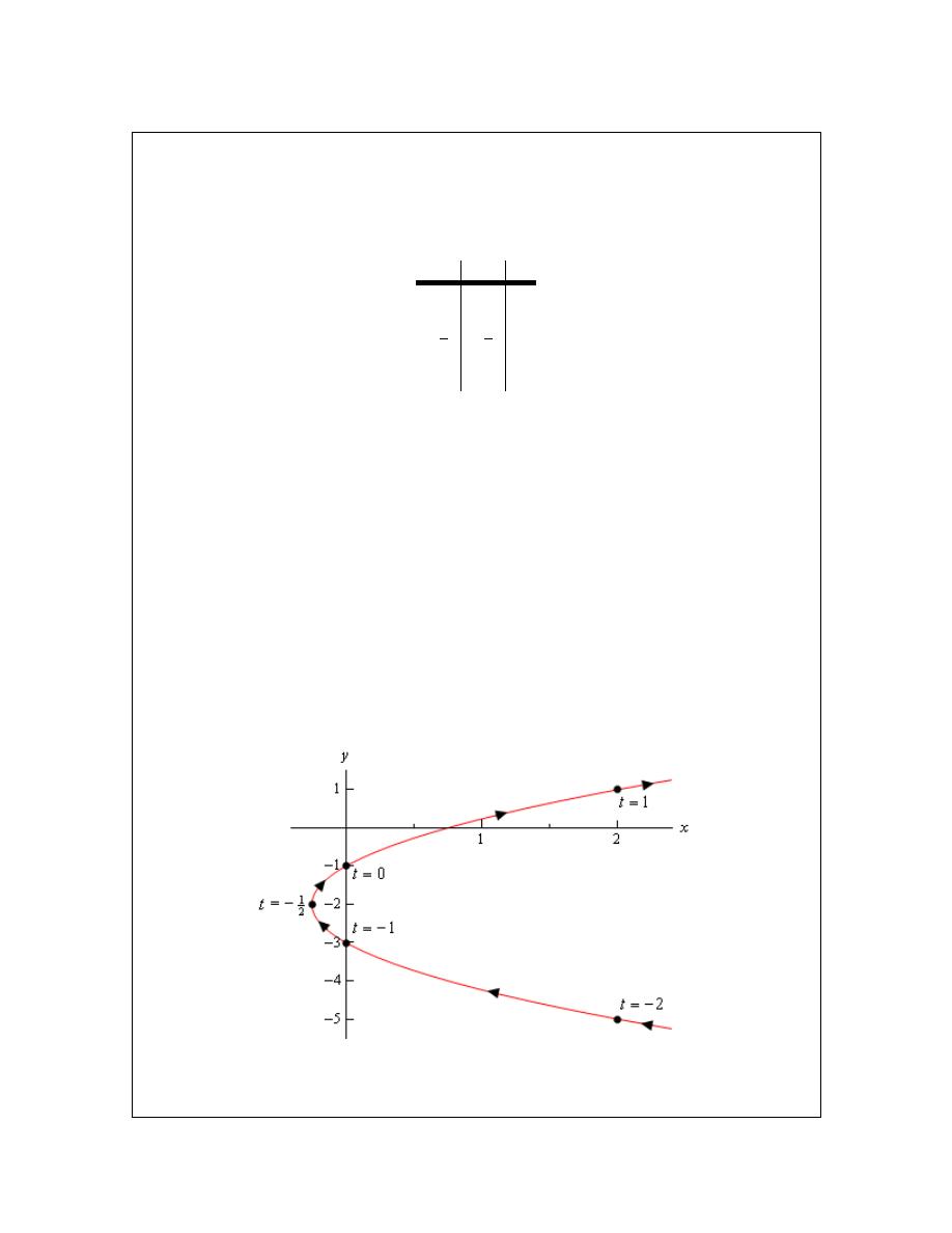
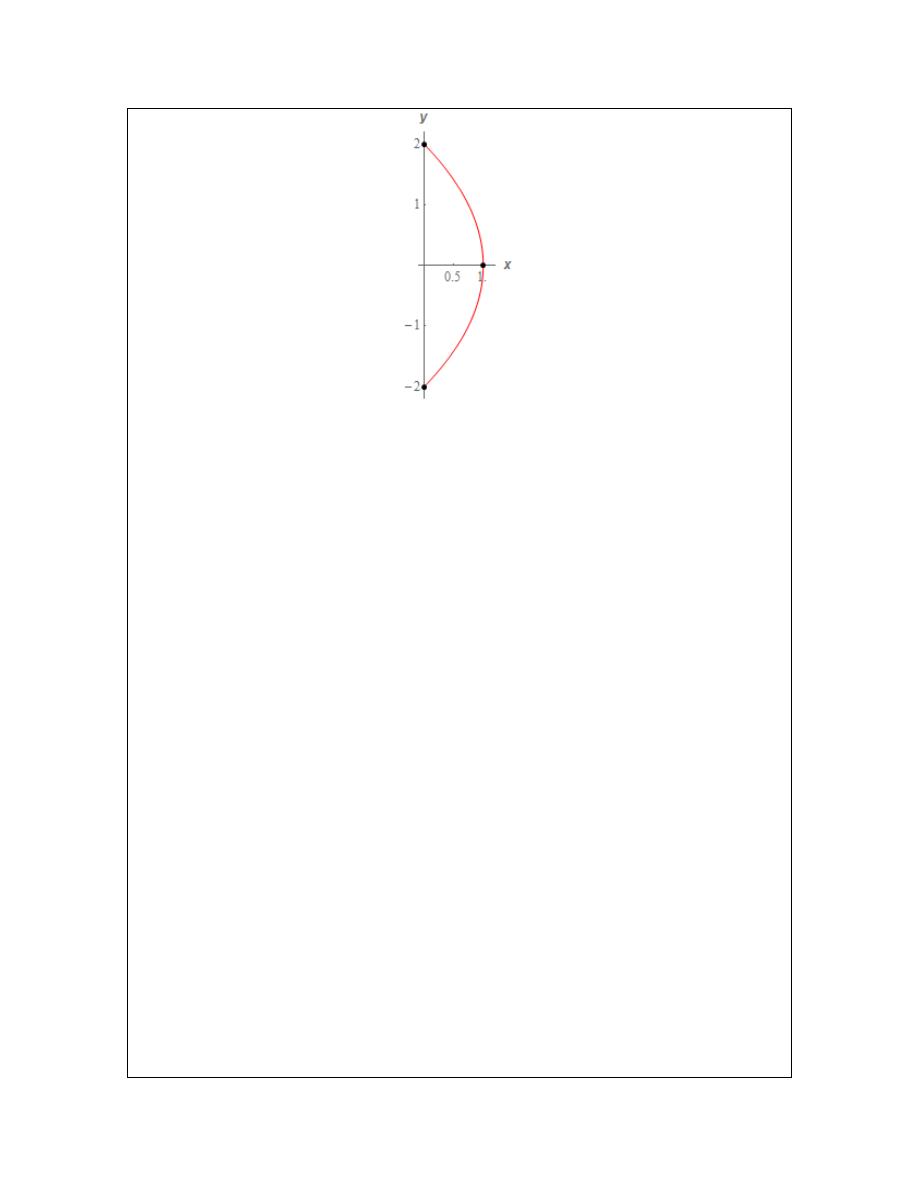
Example 1

Sketch the parametric curve for the following set of parametric equations.

= +

= −

Solution
At this point our only option for sketching a parametric curve is to pick values of t, plug them into
the parametric equations and then plot the points. So, let’s plug in some t’s.

-2

-5

-1

-3

1
2

−

1
4

−

-2

-1

The first question that should be asked at this point is, how did we know to use the values of t that
we did, especially the third choice? Unfortunately, there is no real answer to this question at this
point. We simply pick t’s until we are fairly confident that we’ve got a good idea of what the
curve looks like. It is this problem with picking “good” values of t that make this method of
sketching parametric curves one of the poorer choices. Sometimes we have no choice, but if we
do have a choice we should avoid it.

We’ll discuss an alternate graphing method in later examples that will help to explain how these
values of t were chosen.

We have one more idea to discuss before we actually sketch the curve. Parametric curves have a
direction of motion. The direction of motion is given by increasing t. So, when plotting
parametric curves, we also include arrows that show the direction of motion. We will often give
the value of t that gave specific points on the graph as well to make it clear the value of t that
gave that particular point.

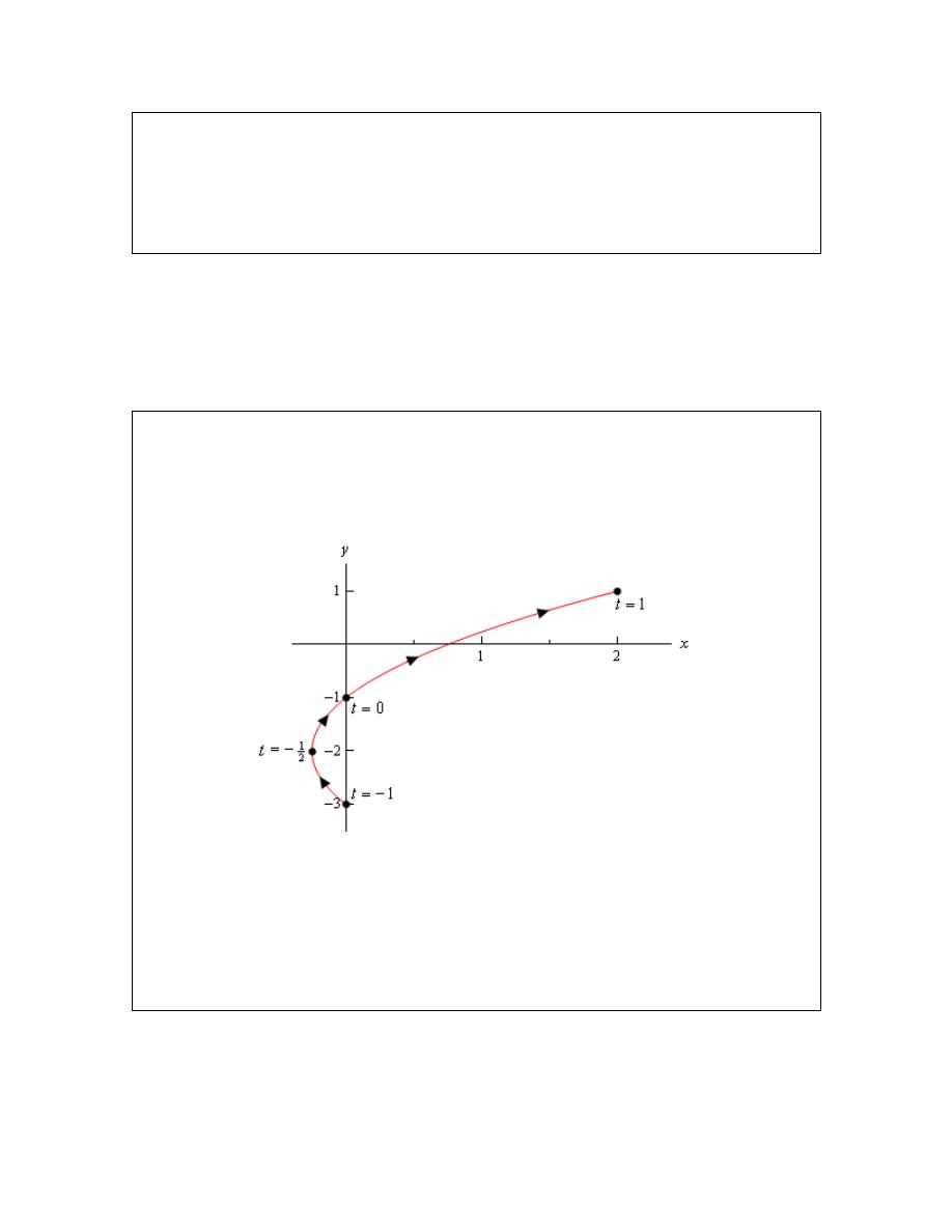
Here is the sketch of this parametric curve.

So, it looks like we have a parabola that opens to the right.

Before we end this example there is a somewhat important and subtle point that we need to

Calculus II

http://tutorial.math.lamar.edu/terms.aspx

discuss first. Notice that we made sure to include a portion of the sketch to the right of the points
corresponding to

= −

and

to indicate that there are portions of the sketch there. Had we

simply stopped the sketch at those points we are indicating that there was no portion of the curve
to the right of those points and there clearly will be. We just didn’t compute any of those points.

This may seem like an unimportant point, but as we’ll see in the next example it’s more important
than we might think.

Before addressing a much easier way to sketch this graph let’s first address the issue of limits on
the parameter.  In the previous example we didn’t have any limits on the parameter.  Without
limits on the parameter the graph will continue in both directions as shown in the sketch above.

We will often have limits on the parameter however and this will affect the sketch of the
parametric equations.  To see this effect let’s look a slight variation of the previous example.

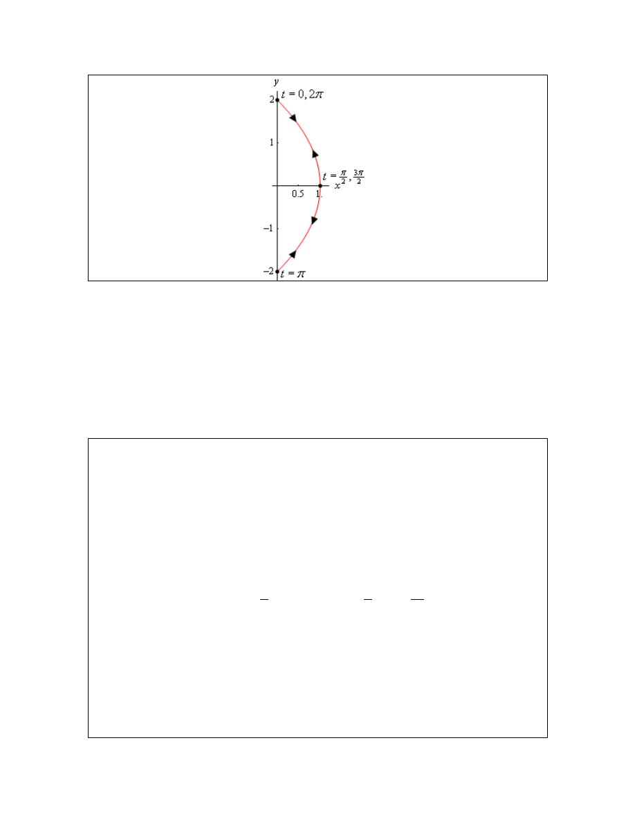
Example 2

Sketch the parametric curve for the following set of parametric equations.

= +

= −

− ≤ ≤

Solution
Note that the only difference here is the presence of the limits on t.  All these limits do is tell us
that we can’t take any value of t outside of this range.  Therefore, the parametric curve will only
be a portion of the curve above.  Here is the parametric curve for this example.

Notice that with this sketch we started and stopped the sketch right on the points originating from
the end points of the range of t’s. Contrast this with the sketch in the previous example where we
had a portion of the sketch to the right of the “start” and “end” points that we computed.

In this case the curve starts at

= −

and ends at

, whereas in the previous example the

curve didn’t really start at the right most points that we computed. We need to be clear in our
sketches if the curve starts/ends right at a point, or if that point was simply the first/last one that
we computed.

It is now time to take a look at an easier method of sketching this parametric curve. This method
uses the fact that in many, but not all, cases we can actually eliminate the parameter from the
parametric equations and get a function involving only x and y. We will sometimes call this the
algebraic equation to differentiate it from the original parametric equations. There will be two

Calculus II

http://tutorial.math.lamar.edu/terms.aspx

small problems with this method, but it will be easy to address those problems. It is important to
note however that we won’t always be able to do this.

Just how we eliminate the parameter will depend upon the parametric equations that we’ve got.
Let’s see how to eliminate the parameter for the set of parametric equations that we’ve been
working with to this point.

Example 3

Eliminate the parameter from the following set of parametric equations.

= +

= −

Solution
One of the easiest ways to eliminate the parameter is to simply solve one of the equations for the
parameter (t, in this case) and substitute that into the other equation. Note that while this may be
the easiest to eliminate the parameter, it’s usually not the best way as we’ll see soon enough.

In this case we can easily solve y for t.

(

)

Plugging this into the equation for x gives the following algebraic equation,

(

)

(

)





+ =

+ +









Sure enough from our Algebra knowledge we can see that this is a parabola that opens to the right

and will have a vertex at

(

)

1
4

, 2

− −

We won’t bother with a sketch for this one as we’ve already sketched this once and the point here
was more to eliminate the parameter anyway.

Before we leave this example let’s address one quick issue.

In the first example we just, seemingly randomly, picked values of t to use in our table, especially
the third value. There really was no apparent reason for choosing

1
2

= −

. It is however

probably the most important choice of t as it is the one that gives the vertex.

The reality is that when writing this material up we actually did this problem first then went back
and did the first problem. Plotting points is generally the way most people first learn how to
construct graphs and it does illustrate some important concepts, such as direction, so it made
sense to do that first in the notes. In practice however, this example is often done first.

So, how did we get those values of t? Well let’s start off with the vertex as that is probably the
most important point on the graph. We have the x and y coordinates of the vertex and we also
have x and y parametric equations for those coordinates. So, plug in the coordinates for the
vertex into the parametric equations and solve for t. Doing this gives,

(

)

1
2

double root

= −

− = +

⇒

= −

− = −

Calculus II

http://tutorial.math.lamar.edu/terms.aspx

So, as we can see, the value of t that will give both of these coordinates is

1
2

= −

. Note that the

x parametric equation gave a double root and this will often not happen. Often we would have
gotten two distinct roots from that equation. In fact, it won’t be unusual to get multiple values of
t from each of the equations.

However, what we can say is that there will be a value(s) of t that occurs in both sets of solutions
and that is the t that we want for that point. We’ll eventually see an example where this happens
in a later section.

Now, from this work we can see that if we use

1
2

= −

we will get the vertex and so we included

that value of t in the table in Example 1. Once we had that value of t we chose two integer values
of t on either side to finish out the table.

As we will see in later examples in this section determining values of t that will give specific
points is something that we’ll need to do on a fairly regular basis. It is fairly simple however as
this example has shown. All we need to be able to do is solve a (usually) fairly basic equation
which by this point in time shouldn’t be too difficult.

Getting a sketch of the parametric curve once we’ve eliminated the parameter seems fairly
simple.  All we need to do is graph the equation that we found by eliminating the parameter.  As
noted already however, there are two small problems with this method.  The first is direction of
motion.  The equation involving only x and y will NOT give the direction of motion of the
parametric curve.  This is generally an easy problem to fix however.  Let’s take a quick look at
the derivatives of the parametric equations from the last example.  They are,

= +

Now, all we need to do is recall our Calculus I knowledge. The derivative of y with respect to t is
clearly always positive. Recalling that one of the interpretations of the first derivative is rate of
change we now know that as t increases y must also increase. Therefore, we must be moving up
the curve from bottom to top as t increases as that is the only direction that will always give an
increasing y as t increases.

Note that the x derivative isn’t as useful for this analysis as it will be both positive and negative
and hence x will be both increasing and decreasing depending on the value of t. That doesn’t help
with direction much as following the curve in either direction will exhibit both increasing and
decreasing x.

In some cases, only one of the equations, such as this example, will give the direction while in
other cases either one could be used. It is also possible that, in some cases, both derivatives
would be needed to determine direction. It will always be dependent on the individual set of
parametric equations.

The second problem with eliminating the parameter is best illustrated in an example as we’ll be
running into this problem in the remaining examples.

Calculus II

http://tutorial.math.lamar.edu/terms.aspx

Example 4

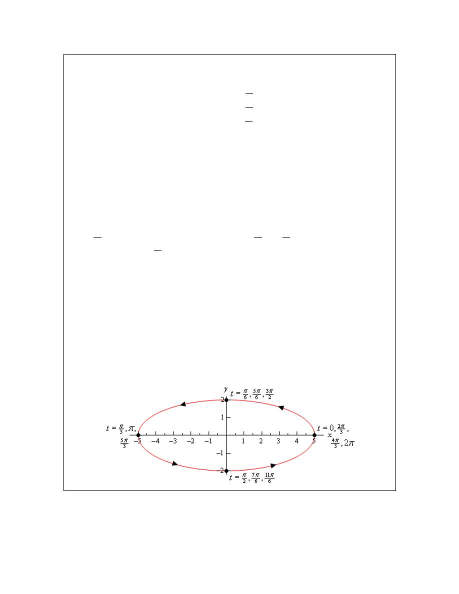
Sketch the parametric curve for the following set of parametric equations. Clearly

indicate direction of motion.

5 cos

2 sin

≤ ≤

Solution
Before we proceed with eliminating the parameter for this problem let’s first address again why
just picking t’s and plotting points is not really a good idea.

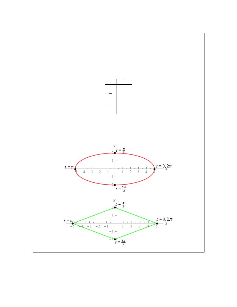
Given the range of t’s in the problem statement let’s use the following set of t’s.

-5

-2

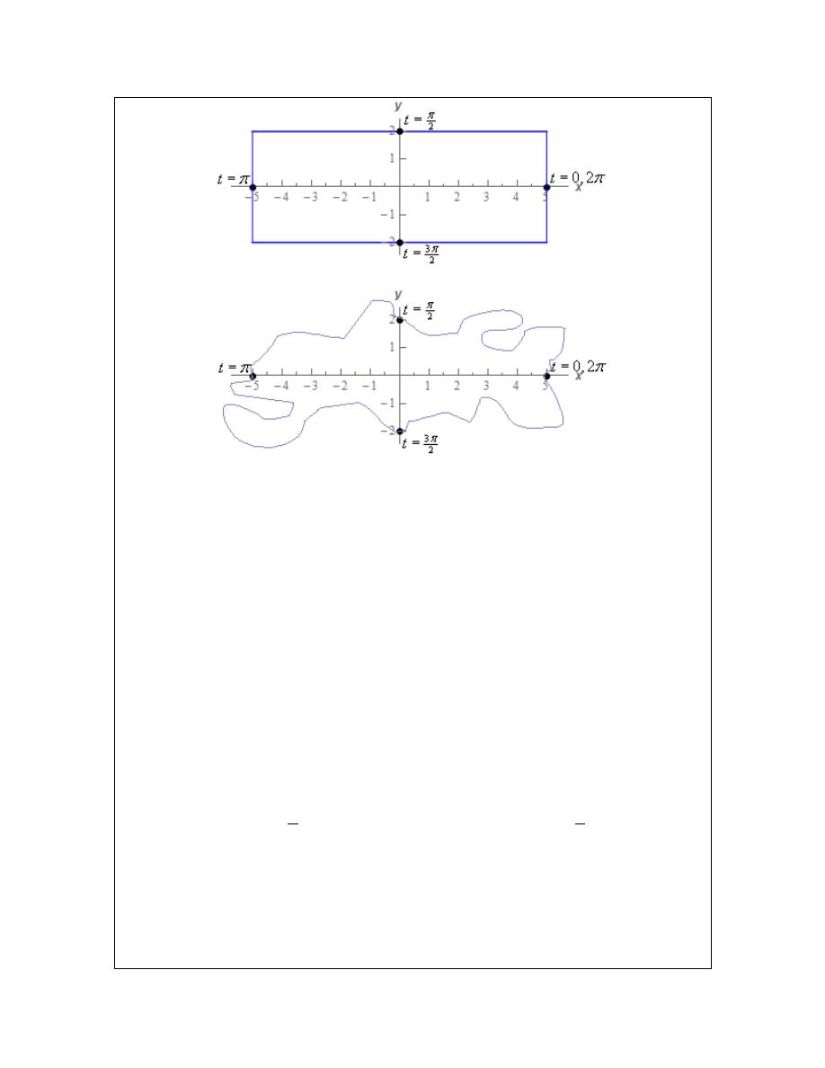
The question that we need to ask now is do we have enough points to accurately sketch the graph
of this set of parametric equations? Below are some sketches of some possible graphs of the
parametric equation based only on these five points.

Calculus II

http://tutorial.math.lamar.edu/terms.aspx

Given the nature of sine/cosine you might be able to eliminate the diamond and the square but
there is no denying that they are graphs that go through the given points. The last graph is also a
little silly but it does show a graph going through the given points.

Again, given the nature of sine/cosine you can probably guess that the correct graph is the ellipse.
However, that is all that would be at this point. A guess. Nothing actually says unequivocally
that the parametric curve is an ellipse just from those five points.  That is the danger of sketching
parametric curves based on a handful of points. Unless we know what the graph will be ahead of
time we are really just making a guess.

So, in general, we should avoid plotting points to sketch parametric curves. The best method,
provided it can be done, is to eliminate the parameter. As noted just prior to starting this example
there is still a potential problem with eliminating the parameter that we’ll need to deal with. We
will eventually discuss this issue. For now, let’s just proceed with eliminating the parameter.

We’ll start by eliminating the parameter as we did in the previous section.  We’ll solve one of the
of the equations for t and plug this into the other equation.  For example, we could do the
following,

cos

2 sin cos

−





 

⇒

 





 





Can you see the problem with doing this?  This is definitely easy to do but we have a greater
chance of correctly graphing the original parametric equations by plotting points than we do
graphing this!

There are many ways to eliminate the parameter from the parametric equations and solving for t
is usually not the best way to do it.  While it is often easy to do we will, in most cases, end up

Calculus II

http://tutorial.math.lamar.edu/terms.aspx

with an equation that is almost impossible to deal with.

So, how can we eliminate the parameter here? In this case all we need to do is recall a very nice
trig identity and the equation of an ellipse. Let’s notice that we could do the following here.

25 cos

4 sin

cos

sin

Eliminating the middle steps gives the following algebraic equation,

and so it looks like we’ve got an ellipse.

Before proceeding with this example it should be noted that what we did was probably not all that
obvious to most. However, once it’s been done it does clearly work and so it’s a nice idea that we
can use to eliminate the parameter from some parametric equations involving sines and cosines.
It won’t always work and sometimes it will take a lot more manipulation of things than we did
here.

An alternate method that we could have used here was to solve the two parametric equations for
sine and cosine as follows,

cos

sin

Then, recall the trig identity we used above and these new equations we get,

cos

sin

 

 

 

So, the same answer as the other method. Which method you use will probably depend on which
you find easier to use. Both are perfectly valid and will get the same result.

Now, let’s continue on with the example. We’ve identified that the parametric equations describe
an ellipse, but we can’t just sketch an ellipse and be done with it.

First, just because the algebraic equation was an ellipse doesn’t actually mean that the parametric
curve is the full ellipse. It is always possible that the parametric curve is only a portion of the
ellipse. In order to identify just how much of the ellipse the parametric curve will cover let’s go
back to the parametric equations and see what they tell us about any limits on x and y. Based on
our knowledge of sine and cosine we have the following,

1 cos

5 cos

1 sin

2 sin

− ≤

≤

⇒

− ≤

≤

⇒

− ≤ ≤

− ≤

≤

⇒

− ≤

≤

⇒

− ≤ ≤

So, by starting with sine/cosine and “building up” the equation for x and y using basic algebraic
manipulations we get that the parametric equations enforce the above limits on x and y. In this
case, these also happen to be the full limits on x and y we get by graphing the full ellipse.

Calculus II

http://tutorial.math.lamar.edu/terms.aspx

This is the second potential issue alluded to above.  The parametric curve may not always trace
out the full graph of the algebraic curve. We should always find limits on x and y enforced upon
us by the parametric curve to determine just how much of the algebraic curve is actually sketched
out by the parametric equations.

Therefore, in this case, we now know that we get a full ellipse from the parametric equations.
Before we proceed with the rest of the example be careful to not always just assume we will get
the full graph of the algebraic equation.  There are definitely times when we will not get the full
graph and we’ll need to do a similar analysis to determine just how much of the graph we actually
get. We’ll see an example of this later.

Note as well that any limits on t given in the problem statement can also affect how much of the
graph of the algebraic equation we get. In this case however, based on the table of values we
computed at the start of the problem we can see that we do indeed get the full ellipse in the range

≤ ≤

. That won’t always be the case however, so pay attention to any restrictions on t that

might exist!

Next, we need to determine a direction of motion for the parametric curve. Recall that all
parametric curves have a direction of motion and the equation of the ellipse simply tells us
nothing about the direction of motion.

To get the direction of motion it is tempting to just use the table of values we computed above to
get the direction of motion.  In this case, we would guess (and yes that is all it is – a guess) that
the curve traces out in a counter-clockwise direction.  We’d be correct. In this case, we’d be
correct! The problem is that tables of values can be misleading when determining a direction of
motion as we’ll see in the next example.

Therefore, it is best to not use a table of values to determine the direction of motion. To correctly
determine the direction of motion we’ll use the same method of determining the direction that we
discussed after Example 3.  In other words, we’ll take the derivative of the parametric equations
and use our knowledge of Calculus I and trig to determine the direction of motion.

The derivatives of the parametric equations are,

5sin

2 cos

= −

Now, at

we are at the point

( )

5, 0

and let’s see what happens if we start increasing t. Let’s

increase t from

. In this range of t’s we know that sine is always positive and so

from the derivative of the x equation we can see that x must be decreasing in this range of t’s.

This, however, doesn’t really help us determine a direction for the parametric curve. Starting at

( )

5, 0

no matter if we move in a clockwise or counter-clockwise direction x will have to decrease

so we haven’t really learned anything from the x derivative.

The derivative from the y parametric equation on the other hand will help us. Again, as we
increase t from

we know that cosine will be positive and so y must be increasing

in this range. That however, can only happen if we are moving in a counter-clockwise direction.

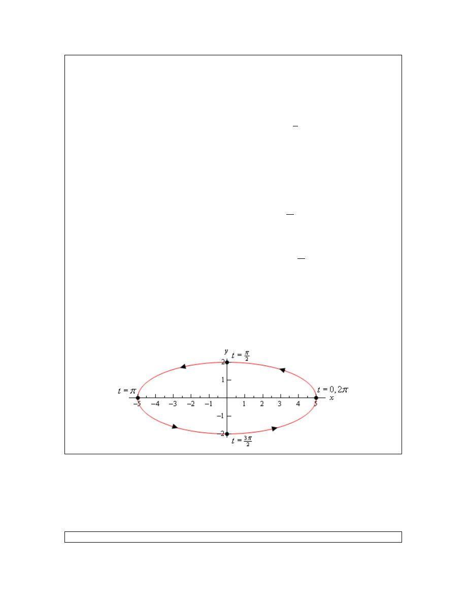
Calculus II

http://tutorial.math.lamar.edu/terms.aspx

If we were moving in a clockwise direction from the point

( )

5, 0

we can see that y would have to

decrease!

Therefore, in the first quadrant we must be moving in a counter-clockwise direction. Let’s move
on to the second quadrant.

So, we are now at the point

( )

0, 2

and we will increase t from

. In this range of t

we know that cosine will be negative and sine will be positive. Therefore, from the derivatives of
the parametric equations we can see that x is still decreasing and y will now be decreasing as well.

In this quadrant the y derivative tells us nothing as y simply must decrease to move from

( )

0, 2

However, in order for x to decrease, as we know it does in this quadrant, the direction must still
be moving a counter-clockwise rotation.

We are now at

(

)

5, 0

−

and we will increase t from

. In this range of t we know

that cosine is negative (and hence y will be decreasing) and sine is also negative (and hence x will
be increasing). Therefore, we will continue to move in a counter-clockwise motion.

For the 4

quadrant we will start at

(

)

0, 2

−

and increase t from

. In this range

of t we know that cosine is positive (and hence y will be increasing) and sine is negative (and
hence x will be increasing). So, as in the previous three quadrants, we continue to move in a
counter-clockwise motion.

At this point we covered the range of t’s we were given in the problem statement and during the
full range the motion was in a counter-clockwise direction.

We can now fully sketch the parametric curve so, here is the sketch.

Okay, that was a really long example. Most of these types of problems aren’t as long. We just
had a lot to discuss in this one so we could get a couple of important ideas out of the way. The
rest of the examples in this section shouldn’t take as long to go through.

Now, let’s take a look at another example that will illustrate an important idea about parametric
equations.

Example 5

Sketch the parametric curve for the following set of parametric equations. Clearly

Calculus II

http://tutorial.math.lamar.edu/terms.aspx

indicate direction of motion.

( )

5 cos 3

2 sin 3

≤ ≤

Solution
Note that the only difference in between these parametric equations and those in Example 4 is
that we replaced the t with 3t. We can eliminate the parameter here using either of the methods
we discussed in the previous example. In this case we’ll do the following,

( )

25 cos

4 sin

cos

sin

So, we get the same ellipse that we did in the previous example. Also note that we can do the
same analysis on the parametric equations to determine that we have exactly the same limits on x
and y. Namely,

− ≤ ≤

It’s starting to look like changing the t into a 3t in the trig equations will not change the
parametric curve in any way. That is not correct however. The curve does change in a small but
important way which we will be discussing shortly.

Before discussing that small change the 3t brings to the curve let’s discuss the direction of motion
for this curve. Despite the fact that we said in the last example that picking values of t and
plugging in to the equations to find points to plot is a bad idea let’s do it any way.

Given the range of t’s from the problem statement the following set looks like a good choice of
t’s to use.

-2

-5

So, the only change to this table of values/points from the last example is all the nonzero y values
changed sign. From a quick glance at the values in this table it would look like the curve, in this
case, is moving in a clockwise direction. But is that correct? Recall we said that these tables of
values can be misleading when used to determine direction and that’s why we don’t use them.

Let’s see if our first impression is correct. We can check our first impression by doing the
derivative work to get the correct direction. Let’s work with just the y parametric equation as the
x will have the same issue that it had in the previous example. The derivative of the y parametric
equation is,

( )

6 cos 3

Calculus II

http://tutorial.math.lamar.edu/terms.aspx

Now, if we start at

as we did in the previous example and start increasing t. At

the

derivative is clearly positive and so increasing t (at least initially) will force y to also be
increasing. The only way for this to happen is if the curve is in fact tracing out in a counter-
clockwise direction initially.

Now, we could continue to look at what happens as we further increase t, but when dealing with a
parametric curve that is a full ellipse (as this one is) and the argument of the trig functions is of
the form nt for any constant n the direction will not change so once we know the initial direction
we know that it will always move in that direction. Note that this is only true for parametric
equations in the form that we have here. We’ll see in later examples that for different kinds of
parametric equations this may no longer be true.

Okay, from this analysis we can see that the curve must be traced out in a counter-clockwise
direction. This is directly counter to our guess from the tables of values above and so we can see
that, in this case, the table would probably have led us to the wrong direction. So, once again,
tables are generally not very reliable for getting pretty much any real information about a
parametric curve other than a few points that must be on the curve. Outside of that the tables are
rarely useful and will generally not be dealt with in further examples.

So, why did our table give an incorrect impression about the direction? Well recall that we
mentioned earlier that the 3t will lead to a small but important change to the curve versus just a t?
Let’s take a look at just what that change is as it will also answer what “went wrong” with our
table of values.

Let’s start by look at

. At

we are at the point

( )

5, 0

and let’s ask ourselves what

values of t put us back at this point. We saw in Example 3 how to determine value(s) of t that put
us at certain points and the same process will work here with a minor modification.

Instead of looking at both the x and y equations as we did in that example let’s just look at the x
equation. The reason for this is that we’ll note that there are two points on the ellipse that will

have a y coordinate of zero,

( )

5, 0

and

(

)

5, 0

−

. If we set the y coordinate equal to zero we’ll

find all the t’s that are at both of these points when we only want the values of t that are at

( )

5, 0

So, because the x coordinate of five will only occur at this point we can simply use the x
parametric equation to determine the values of t that will put us at this point. Doing this gives the
following equation and solution,

( )

2
3

5 cos 3

cos

0 2

0, 1, 2, 3,

−

=
=

= +

→

= ± ± ± 

Don’t forget that when solving a trig equation we need to add on the “

2 n

” where n represents

the number of full revolutions in the counter-clockwise direction (positive n) and clockwise
direction (negative n) that we rotate from the first solution to get all possible solutions to the
equation.

Now, let’s plug in a few values of n starting at

. We don’t need negative n in this case

since all of those would result in negative t and those fall outside of the range of t’s we were

Calculus II

http://tutorial.math.lamar.edu/terms.aspx

given in the problem statement. The first few values of t are then,

We can stop here as all further values of t will be outside the range of t’s given in this problem.

So, what is this telling us? Well back in Example 4 when the argument was just t the ellipse was
traced out exactly once in the range

≤ ≤

. However, when we change the argument to 3t

(and recalling that the curve will always be traced out in a counter-clockwise direction for this

problem) we are going through the “starting” point of

( )

5, 0

two more times than we did in the

previous example.

In fact, this curve is tracing out three separate times. The first trace is completed in the range

≤ ≤

. The second trace is completed in the range

≤ ≤

and the third and final trace

is completed in the range

≤ ≤

. In other words, changing the argument from t to 3t

increase the speed of the trace and the curve will now trace out three times in the range

≤ ≤

This is why the table gives the wrong impression.  The speed of the tracing has increased leading
to an incorrect impression from the points in the table.  The table seems to suggest that between
each pair of values of t a quarter of the ellipse is traced out in the clockwise direction when in
reality it is tracing out three quarters of the ellipse in the counter-clockwise direction.

Here’s a final sketch of the curve and note that it really isn’t all that different from the previous
sketch.  The only differences are the values of t and the various points we included. We did
include a few more values of t at various points just to illustrate where the curve is at for various
values of t but in general these really aren’t needed.

So, we saw in the last two examples two sets of parametric equations that in some way gave the
same graph. Yet, because they traced out the graph a different number of times we really do need
to think of them as different parametric curves at least in some manner. This may seem like a
difference that we don’t need to worry about, but as we will see in later sections this can be a very

Calculus II

http://tutorial.math.lamar.edu/terms.aspx

important difference. In some of the later sections we are going to need a curve that is traced out
exactly once.

Before we move on to other problems let’s briefly acknowledge what happens by changing the t
to an nt in these kinds of parametric equations. When we are dealing with parametric equations
involving only sines and cosines and they both have the same argument if we change the
argument from t to nt we simply change the speed with which the curve is traced out. If

will increase the speed and if

we will decrease the speed.

Let’s take a look at a couple more examples.

Example 6

Sketch the parametric curve for the following set of parametric equations. Clearly

identify the direction of motion. If the curve is traced out more than once give a range of the
parameter for which the curve will trace out exactly once.

sin

2 cos

Solution
We can eliminate the parameter much as we did in the previous two examples. However, we’ll

need to note that the x already contains a

sin t

and so we won’t need to square the x. We will

however, need to square the y as we need in the previous two examples.

sin

cos

⇒

= −

In this case the algebraic equation is a parabola that opens to the left.

We will need to be very, very careful however in sketching this parametric curve. We will NOT
get the whole parabola. A sketch of the algebraic form parabola will exist for all possible values
of y. However, the parametric equations have defined both x and y in terms of sine and cosine
and we know that the ranges of these are limited and so we won’t get all possible values of x and
y here. So, first let’s get limits on x and y as we did in previous examples. Doing this gives,

1 sin

sin

1 cos

2 cos

− ≤

≤

⇒

≤

⇒

≤ ≤

− ≤

≤

⇒

− ≤

≤

⇒

− ≤ ≤

So, it is clear from this that we will only get a portion of the parabola that is defined by the
algebraic equation. Below is a quick sketch of the portion of the parabola that the parametric
curve will cover.

Calculus II

http://tutorial.math.lamar.edu/terms.aspx

To finish the sketch of the parametric curve we also need the direction of motion for the curve.
Before we get to that however, let’s jump forward and determine the range of t’s for one trace.
To do this we’ll need to know the t’s that put us at each end point and we can follow the same
procedure we used in the previous example. The only difference is this time let’s use the y
parametric equation instead of the x because the y coordinates of the two end points of the curve
are different whereas the x coordinates are the same.

So, for the top point we have,

( )

2 cos

cos

0 2

0, 1, 2, 3,

−

=
=

= +

= ± ± ± 

For, plugging in some values of n we get that the curve will be at the top point at,

, 4 , 2 , 0, 2 , 4 ,

π π

−



Similarly, for the bottom point we have,

( )

2 cos

cos

0, 1, 2, 3,

−

− =

− = +

= ± ± ± 

So, we see that we will be at the bottom point at,

, 3 ,

, , 3 ,

π π π π

−



So, if we start at say,

, we are at the top point and we increase t we have to move along the

curve downwards until we reach

at which point we are now at the bottom point. This

means that we will trace out the curve exactly once in the range

≤ ≤

This is not the only range that will trace out the curve however. Note that if we further increase t
from

we will now have to travel back up the curve until we reach

and we are now

back at the top point. Increasing t again until we reach

will take us back down the curve

Calculus II

http://tutorial.math.lamar.edu/terms.aspx

until we reach the bottom point again, etc. From this analysis we can get two more ranges of t for
one trace,

≤ ≤

As you can probably see there are an infinite number of ranges of t we could use for one trace of
the curve. Any of them would be acceptable answers for this problem.

Note that in the process of determining a range of t’s for one trace we also managed to determine
the direction of motion for this curve. In the range

≤ ≤

we had to travel downwards along

the curve to get from the top point at

to the bottom point at

. However, at

are back at the top point on the curve and to get there we must travel along the path. We can’t
just jump back up to the top point or take a different path to get there. All travel must be done on
the path sketched out. This means that we had to go back up the path. Further increasing t takes
us back down the path, then up the path again etc.

In other words, this path is sketched out in both directions because we are not putting any
restrictions on the t’s and so we have to assume we are using all possible values of t. If we had
put restrictions on which t’s to use we might really have ended up only moving in one direction.
That however would be a result only of the range of t’s we are using and not the parametric
equations themselves.

Note that we didn’t really need to do the above work to determine that the curve traces out in both
directions.in this case. Both the x and y parametric equations involve sine or cosine and we know
both of those functions oscillate. This, in turn means that both x and y will oscillate as well. The
only way for that to happen on this particular this curve will be for the curve to be traced out in
both directions.

Be careful with the above reasoning that the oscillatory nature of sine/cosine forces the curve to
be traced out in both directions. It can only be used in this example because the “starting” point
and “ending” point of the curves are in different places. The only way to get from one of the
“end” points on the curve to the other is to travel back along the curve in the opposite direction.

Contrast this with the ellipse in Example 4. In that case we had sine/cosine in the parametric
equations as well. However, the curve only traced out in one direction, not in both directions. In
Example 4 we were graphing the full ellipse and so no matter where we start sketching the graph
we will eventually get back to the “starting” point without ever retracing any portion of the graph.
In Example 4 as we trace out the full ellipse both x and y do in fact oscillate between their two
“endpoints” but the curve itself does not trace out in both directions for this to happen.

Basically, we can only use the oscillatory nature of sine/cosine to determine that the curve traces
out in both directions if the curve starts and ends at different points. If the starting/ending point is
the same then we generally need to go through the full derivative argument to determine the
actual direction of motion.

So, to finish this problem out, below is a sketch of the parametric curve. Note that we put
direction arrows in both directions to clearly indicate that it would be traced out in both
directions. We also put in a few values of t just to help illustrate the direction of motion.

Calculus II

http://tutorial.math.lamar.edu/terms.aspx

To this point we’ve seen examples that would trace out the complete graph that we got by
eliminating the parameter if we took a large enough range of t’s. However, in the previous
example we’ve now seen that this will not always be the case. It is more than possible to have a
set of parametric equations which will continuously trace out just a portion of the curve. We can
usually determine if this will happen by looking for limits on x and y that are imposed up us by
the parametric equation.

We will often use parametric equations to describe the path of an object or particle. Let’s take a
look at an example of that.

Example 7

The path of a particle is given by the following set of parametric equations.

( )

3cos 2

1 cos

= +

Completely describe the path of this particle. Do this by sketching the path, determining limits on
x and y and giving a range of t’s for which the path will be traced out exactly once (provide it
traces out more than once of course).

Solution
Eliminating the parameter this time will be a little different. We only have cosines this time and
we’ll use that to our advantage. We can solve the x equation for cosine and plug that into the
equation for y. This gives,

( )

cos 2

 

= +

 

 

This time the algebraic equation is a parabola that opens upward. We also have the following
limits on x and y.

( )

1 cos 2

3cos 2

cos

1 1 cos

− ≤

≤

− ≤

≤

− ≤ ≤

≤

≤ +

≤

≤ ≤

So, again we only trace out a portion of the curve. Here is a quick sketch of the portion of the
parabola that the parametric curve will cover.

Calculus II

http://tutorial.math.lamar.edu/terms.aspx

Now, as we discussed in the previous example because both the x and y parametric equations
involve cosine we know that both x and y must oscillate and because the “start” and “end” points
of the curve are not the same the only way x and y can oscillate is for the curve to trace out in
both directions.

To finish the problem then all we need to do is determine a range of t’s for one trace. Because the
“end” points on the curve have the same y value and different x values we can use the x
parametric equation to determine these values. Here is that work.

( )

3 :

3cos 2

cos 2

0 2

0, 1, 2, 3,

= +

→

= ± ± ± 

( )

1
2

3 :

3cos 2

cos 2

0, 1, 2, 3,

π π

= −

− =
− =

= +

→

= ± ± ± 

So, we will be at the right end point at

, 2 ,

, 0, , 2 ,

π π

−



and we’ll be at the left end

point at

π π π

−



. So, in this case there are an infinite number of ranges of

t’s for one trace. Here are a few of them.

−

≤ ≤

Here is a final sketch of the particle’s path with a few value of t on it.

Calculus II

http://tutorial.math.lamar.edu/terms.aspx

We should give a small warning at this point. Because of the ideas involved in them we
concentrated on parametric curves that retraced portions of the curve more than once. Do not,
however, get too locked into the idea that this will always happen.  Many, if not most parametric
curves will only trace out once.  The first one we looked at is a good example of this.  That
parametric curve will never repeat any portion of itself.

There is one final topic to be discussed in this section before moving on. So far we’ve started
with parametric equations and eliminated the parameter to determine the parametric curve.

However, there are times in which we want to go the other way. Given a function or equation we
might want to write down a set of parametric equations for it.  In these cases we say that we
parameterize the function.

If we take Examples 4 and 5 as examples we can do this for ellipses (and hence circles). Given
the ellipse

a set of parametric equations for it would be,

cos

sin

This set of parametric equations will trace out the ellipse starting at the point

( )

, 0

and will trace

in a counter-clockwise direction and will trace out exactly once in the range

≤ ≤

. This is

a fairly important set of parametric equations as it used continually in some subjects with dealing
with ellipses and/or circles.

Every curve can be parameterized in more than one way. Any of the following will also
parameterize the same ellipse.

( )

cos

sin

cos

sin

= −

The presence of the

will change the speed that the ellipse rotates as we saw in Example 5.

Note as well that the last two will trace out ellipses with a clockwise direction of motion (you
might want to verify this). Also note that they won’t all start at the same place (if we think of

as the starting point that is).

There are many more parameterizations of an ellipse of course, but you get the idea. It is
important to remember that each parameterization will trace out the curve once with a potentially
different range of t’s. Each parameterization may rotate with different directions of motion and
may start at different points.

You may find that you need a parameterization of an ellipse that starts at a particular place and
has a particular direction of motion and so you now know that with some work you can write
down a set of parametric equations that will give you the behavior that you’re after.

Now, let’s write down a couple of other important parameterizations and all the comments about
direction of motion, starting point, and range of t’s for one trace (if applicable) are still true.

Calculus II

http://tutorial.math.lamar.edu/terms.aspx

First, because a circle is nothing more than a special case of an ellipse we can use the
parameterization of an ellipse to get the parametric equations for a circle centered at the origin of
radius r as well. One possible way to parameterize a circle is,

cos

sin

Finally, even though there may not seem to be any reason to, we can also parameterize functions

in the form

( )

f x

( )

h y

. In these cases we parameterize them in the following way,

( )

h t

f t

At this point it may not seem all that useful to do a parameterization of a function like this, but
there are many instances where it will actually be easier, or it may even be required, to work with
the parameterization instead of the function itself. Unfortunately, almost all of these instances
occur in a Calculus III course.

Calculus II

http://tutorial.math.lamar.edu/terms.aspx

Tangents with Parametric Equations

In this section we want to find the tangent lines to the parametric equations given by,

( )

f t

g t

To do this let’s first recall how to find the tangent line to

( )

F x

. Here the tangent

line is given by,

( )

(

)

( )

, where

x a

F a

m x a

F a

′

−

Now, notice that if we could figure out how to get the derivative

from the parametric

equations we could simply reuse this formula since we will be able to use the parametric
equations to find the x and y coordinates of the point.

So, just for a second let’s suppose that we were able to eliminate the parameter from the

parametric form and write the parametric equations in the form

( )

F x

. Now, plug the

parametric equations in for x and y. Yes, it seems silly to eliminate the parameter, then
immediately put it back in, but it’s what we need to do in order to get our hands on the derivative.
Doing this gives,

( )

(

)

g t

F f t

Now, differentiate with respect to t and notice that we’ll need to use the Chain Rule on the right
hand side.

( )

(

)

( )

g t

f t

′

Let’s do another change in notation. We need to be careful with our derivatives here.
Derivatives of the lower case function are with respect to t while derivatives of upper case
functions are with respect to x. So, to make sure that we keep this straight let’s rewrite things as
follows.

( )

F x

′

At this point we should remind ourselves just what we are after. We needed a formula for

( )

F x

′

that is in terms of the parametric formulas. Notice however that we can get that from the

above equation.

, provided

≠

Notice as well that this will be a function of t and not x.

Calculus II

http://tutorial.math.lamar.edu/terms.aspx

As an aside, notice that we could also get the following formula with a similar derivation if we
needed to,

Derivative for Parametric E quations

, provided

≠

Why would we want to do this? Well, recall that in the

arc length

section of the Applications of

Integral section we actually needed this derivative on occasion.

So, let’s find a tangent line.

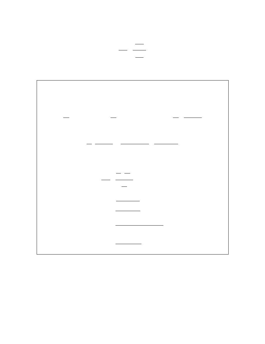
Example 1

Find the tangent line(s) to the parametric curve given by

= −

at (0,4).

Solution
Note that there is apparently the potential for more than one tangent line here! We will look into
this more after we’re done with the example.

The first thing that we should do is find the derivative so we can get the slope of the tangent line.

−

At this point we’ve got a small problem. The derivative is in terms of t and all we’ve got is an x-y
coordinate pair. The next step then is to determine the value(s) of t which will give this point.
We find these by plugging the x and y values into the parametric equations and solving for t.

(

)

0, 2

= −

−

⇒

= ±

⇒

= ±

Any value of t which appears in both lists will give the point. So, since there are two values of t
that give the point we will in fact get two tangent lines. That’s definitely not something that
happened back in Calculus I and we’re going to need to look into this a little more. However,
before we do that let’s actually get the tangent lines.

t = –2
Since we already know the x and y-coordinates of the point all that we need to do is find the slope
of the tangent line.

=−

= −

Calculus II

http://tutorial.math.lamar.edu/terms.aspx

The tangent line (at t = –2) is then,

= −

t = 2
Again, all we need is the slope.

The tangent line (at t = 2) is then,

= +

Now, let’s take a look at just how we could possibly get two tangents lines at a point. This was
definitely not possible back in Calculus I where we first ran across tangent lines.

A quick graph of the parametric curve will explain what is going on here.

So, the parametric curve crosses itself!  That explains how there can be more than one tangent
line.  There is one tangent line for each instance that the curve goes through the point.

The next topic that we need to discuss in this section is that of horizontal and vertical tangents.
We can easily identify where these will occur (or at least the t’s that will give them) by looking at
the derivative formula.

Horizontal tangents will occur where the derivative is zero and that means that we’ll get
horizontal tangent at values of t for which we have,

Calculus II

http://tutorial.math.lamar.edu/terms.aspx

Horizontal Tangent for Parametric Equations

0, provided

≠

Vertical tangents will occur where the derivative is not defined and so we’ll get vertical tangents
at values of t for which we have,

Vertical Tangent for Parametric Equations

0, provided

≠

Let’s take a quick look at an example of this.

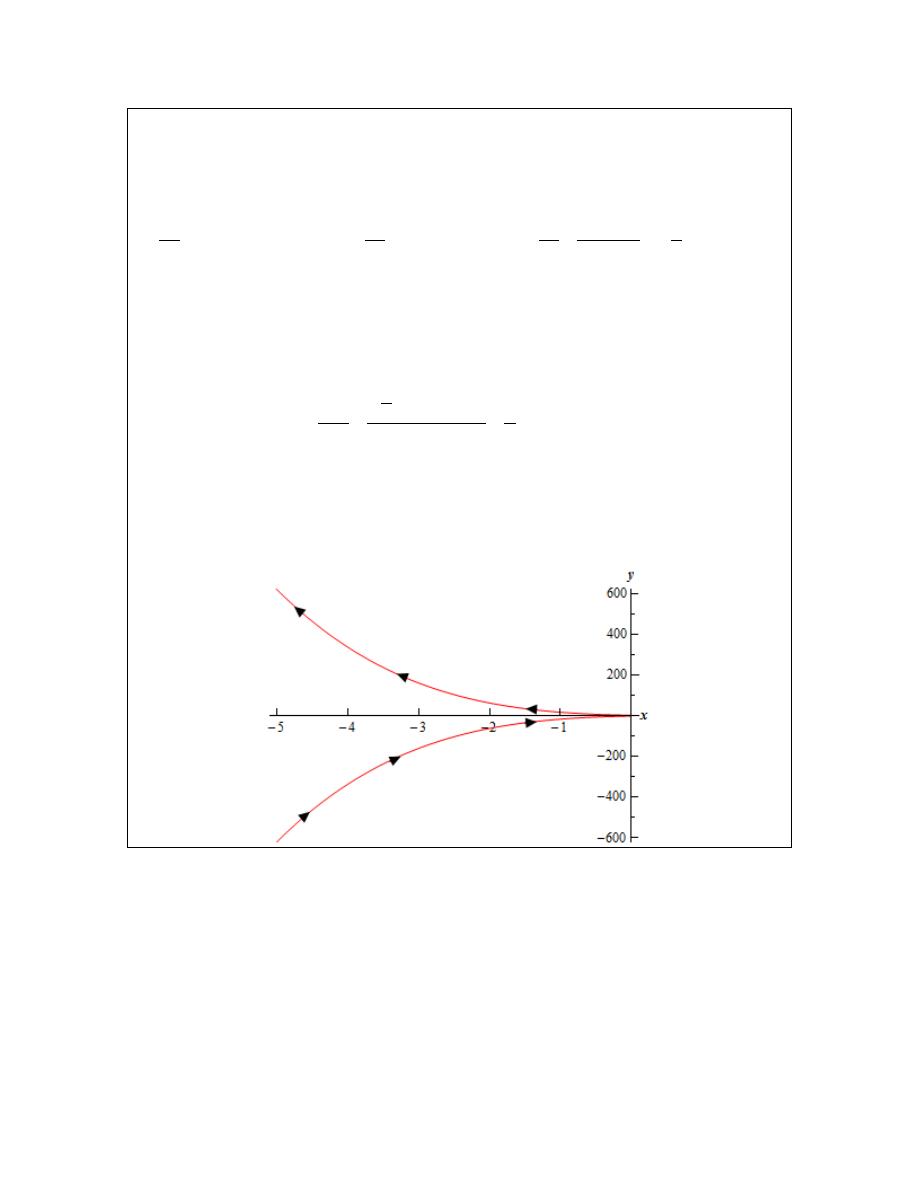
Example 2

Determine the x-y coordinates of the points where the following parametric

equations will have horizontal or vertical tangents.

= −

−

Solution
We’ll first need the derivatives of the parametric equations.

(

)

− =

−

Horizontal Tangents
We’ll have horizontal tangents where,

⇒

Now, this is the value of t which gives the horizontal tangents and we were asked to find the x-y
coordinates of the point. To get these we just need to plug t into the parametric equations.
Therefore, the only horizontal tangent will occur at the point (0,-9).

Vertical Tangents
In this case we need to solve,

(

)

− =

⇒

= ±

The two vertical tangents will occur at the points (2,-6) and (-2,-6).

For the sake of completeness and at least partial verification here is the sketch of the parametric
curve.

Calculus II

http://tutorial.math.lamar.edu/terms.aspx

The final topic that we need to discuss in this section really isn’t related to tangent lines, but does
fit in nicely with the derivation of the derivative that we needed to get the slope of the tangent
line.

Before moving into the new topic let’s first remind ourselves of the formula for the first
derivative and in the process rewrite it slightly.

( )

Written in this way we can see that the formula actually tells us how to differentiate a function y
(as a function of t) with respect to x (when x is also a function of t) when we are using parametric
equations.

Now let’s move onto the final topic of this section. We would also like to know how to get the
second derivative of y with respect to x.

d y

Getting a formula for this is fairly simple if we remember the rewritten formula for the first
derivative above.

Second Derivative for Parametric Equations

d y

dt dx

dx dx

























Calculus II

http://tutorial.math.lamar.edu/terms.aspx

Note that,

d y

d x

≠

Let’s work a quick example.

Example 3

Find the second derivative for the following set of parametric equations.

= −

Solution
This is the set of parametric equations that we used in the first example and so we already have
the following computations completed.

−

We will first need the following,

(

)

(

)

(

)

2 15

24 30

−



 =





−





−

The second derivative is then,

(

)

(

)(

)

(

)

24 30

d y

dt dx













−

So, why would we want the second derivative? Well, recall from your Calculus I class that with
the second derivative we can determine where a curve is concave up and concave down. We
could do the same thing with parametric equations if we wanted to.

Calculus II

http://tutorial.math.lamar.edu/terms.aspx

Example 4

Determine the values of t for which the parametric curve given by the following set

of parametric equations is concave up and concave down.

= −

= +

Solution
To compute the second derivative we’ll first need the following.

(

)

= −

−

Note that we can also use the first derivative above to get some information about the
increasing/decreasing nature of the curve as well. In this case it looks like the parametric curve
will be increasing if

and decreasing if

Now let’s move on to the second derivative.

(

)

(

)

d y

−

It’s clear, hopefully, that the second derivative will only be zero at

. Using this we can see

that the second derivative will be negative if

and positive if

. So the parametric curve

will be concave down for

and concave up for

Here is a sketch of the curve for completeness sake.

Calculus II

http://tutorial.math.lamar.edu/terms.aspx

Area with Parametric Equations

In this section we will find a formula for determining the area under a parametric curve given by
the parametric equations,

( )

f t

g t

We will also need to further add in the assumption that the curve is traced out exactly once as t
increases from

We will do this in much the same way that we found the first derivative in the previous section.

We will first recall how to find the area under

( )

F x

≤ ≤

( )

F x dx

∫

We will now think of the parametric equation

( )

f t

as a substitution in the integral. We will

also assume that

( )

and

( )

for the purposes of this formula. There is actually no

reason to assume that this will always be the case and so we’ll give a corresponding formula later

if it’s the opposite case (

( )

and

( )

So, if this is going to be a substitution we’ll need,

( )

t dt

′

Plugging this into the area formula above and making sure to change the limits to their
corresponding t values gives us,

( )

(

)

( )

F f t

t dt

′

∫

Since we don’t know what F(x) is we’ll use the fact that

( )

(

)

( )

F x

F f t

g t

and we arrive at the formula that we want.

Area Under Parametric Curve, Formula I

( ) ( )

g t f

t dt

′

∫

Now, if we should happen to have

( )

and

( )

the formula would be,

Area Under Parametric Curve, Formula II

( ) ( )

g t f

t dt

′

∫

Let’s work an example.

Calculus II

http://tutorial.math.lamar.edu/terms.aspx

Example 1

Determine the area under the parametric curve given by the following parametric

equations.

(

)

(

)

sin

6 1 cos

−

≤ ≤

Solution
First, notice that we’ve switched the parameter to

for this problem. This is to make sure that

we don’t get too locked into always having t as the parameter.

Now, we could graph this to verify that the curve is traced out exactly once for the given range if
we wanted to. We are going to be looking at this curve in more detail after this example so we
won’t sketch its graph here.

There really isn’t too much to this example other than plugging the parametric equations into the
formula. We’ll first need the derivative of the parametric equation for x however.

(

)

6 1 cos

−

The area is then,

(

)

( )

36 1 cos

1 2 cos

cos

2 cos

cos 2

2 sin

sin 2

108

θ θ

−





−









⌠



⌡

∫

The parametric curve (without the limits) we used in the previous example is called a cycloid. In
its general form the cycloid is,

(

)

(

)

sin

1 cos

−

The cycloid represents the following situation. Consider a wheel of radius r. Let the point where
the wheel touches the ground initially be called P. Then start rolling the wheel to the right. As
the wheel rolls to the right trace out the path of the point P. The path that the point P traces out is
called a cycloid and is given by the equations above. In these equations we can think of

as the

angle through which the point P has rotated.

Here is a cycloid sketched out with the wheel shown at various places. The blue dot is the point
P on the wheel that we’re using to trace out the curve.

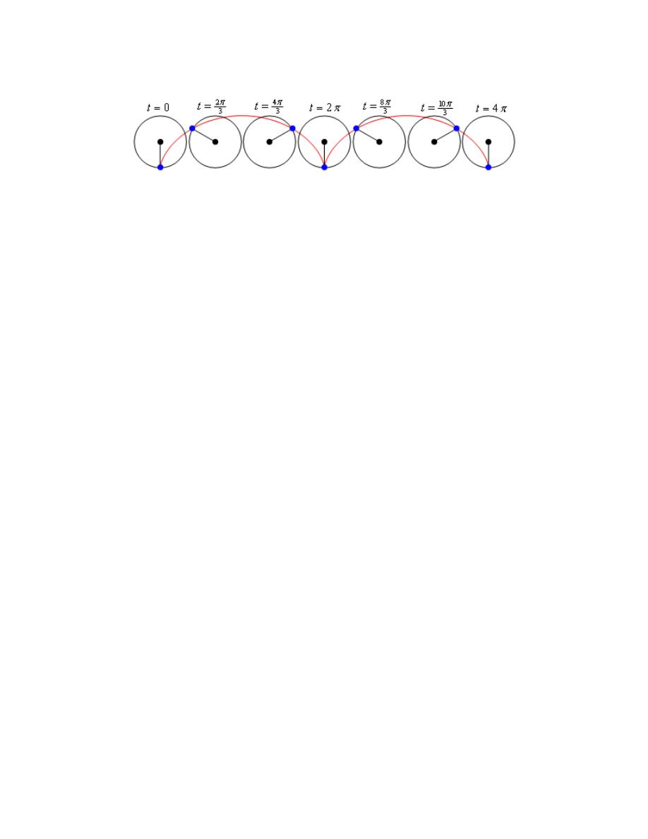
Calculus II

http://tutorial.math.lamar.edu/terms.aspx

From this sketch we can see that one arch of the cycloid is traced out in the range

≤ ≤

This makes sense when you consider that the point P will be back on the ground after it has
rotated through an angle of 2

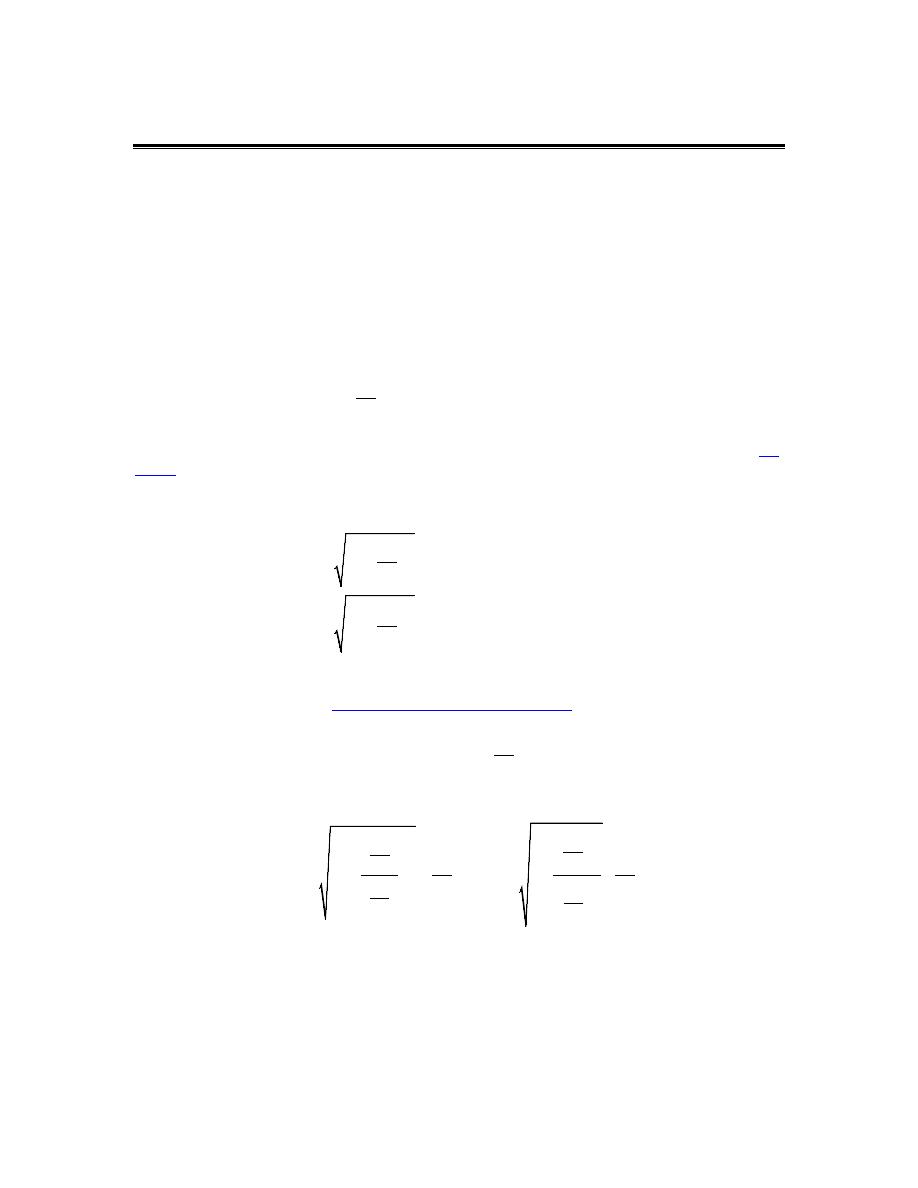
Calculus II

http://tutorial.math.lamar.edu/terms.aspx

Arc Length with Parametric Equations

In the previous two sections we’ve looked at a couple of Calculus I topics in terms of parametric
equations. We now need to look at a couple of Calculus II topics in terms of parametric
equations.

In this section we will look at the arc length of the parametric curve given by,

( )

f t

g t

≤ ≤

We will also be assuming that the curve is traced out exactly once as t increases from

. We

will also need to assume that the curve is traced out from left to right as t increases. This is
equivalent to saying,

for

≥

≤ ≤

So, let’s start out the derivation by recalling the arc length formula as we first derived it in the

arc

length

section of the Applications of Integrals chapter.

∫

where,

( )

if ,

f x

h y





≤ ≤













≤ ≤









We will use the first ds above because we have a nice formula for the derivative in terms of the
parametric equations (see the

Tangents with Parametric Equations

section). To use this we’ll also

need to know that,

( )

t dt

′

The arc length formula then becomes,













































⌠



⌡

This is a particularly unpleasant formula. However, if we factor out the denominator from the
square root we arrive at,

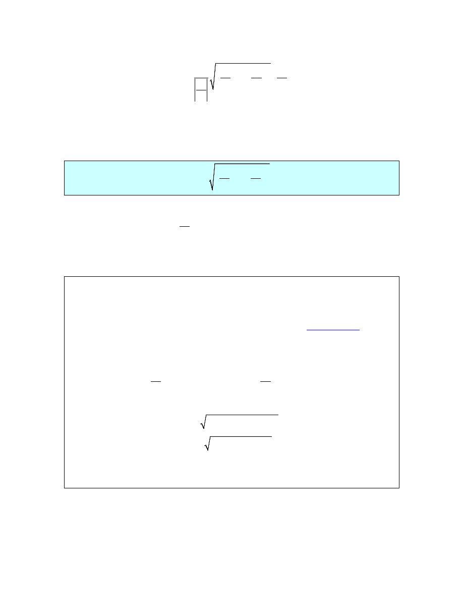
Calculus II

http://tutorial.math.lamar.edu/terms.aspx

























⌠



⌡

Now, making use of our assumption that the curve is being traced out from left to right we can
drop the absolute value bars on the derivative which will allow us to cancel the two derivatives
that are outside the square root and this gives,

Arc Length for Parametric Equations

























⌠



⌡

Notice that we could have used the second formula for ds above if we had assumed instead that

for

≥

≤ ≤

If we had gone this route in the derivation we would have gotten the same formula.

Let’s take a look at an example.

Example 1

Determine the length of the parametric curve given by the following parametric

equations.

( )

3sin

3cos

≤ ≤

Solution
We know that this is a circle of radius 3 centered at the origin from our

prior discussion

about

graphing parametric curves. We also know from this discussion that it will be traced out exactly
once in this range.

So, we can use the formula we derived above. We’ll first need the following,

( )

3cos

3sin

= −

The length is then,

( )

9 sin

9 cos

3 sin

cos

t dt

∫
∫

∫

Since this is a circle we could have just used the fact that the length of the circle is just the
circumference of the circle. This is a nice way, in this case, to verify our result.

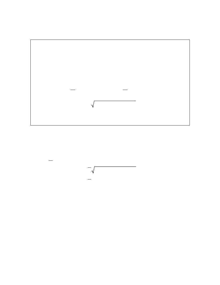
Calculus II

http://tutorial.math.lamar.edu/terms.aspx

Let’s take a look at one possible consequence if a curve is traced out more than once and we try
to find the length of the curve without taking this into account.

Example 2

Use the arc length formula for the following parametric equations.

( )

3sin 3

3cos 3

≤ ≤

Solution
Notice that this is the identical circle that we had in the previous example and so the length is still
6

. However, for the range given we know it will trace out the curve three times instead once as

required for the formula. Despite that restriction let’s use the formula anyway and see what
happens.

In this case the derivatives are,

( )

9 cos 3

9 sin 3

= −

and the length formula gives,

( )

81sin

81cos

t dt

∫
∫

The answer we got form the arc length formula in this example was 3 times the actual length.
Recalling that we also determined that this circle would trace out three times in the range given,
the answer should make some sense.

If we had wanted to determine the length of the circle for this set of parametric equations we
would need to determine a range of t for which this circle is traced out exactly once. This
is,

≤ ≤

. Using this range of t we get the following for the length.

( )

81sin

81cos

t dt

∫
∫

which is the correct answer.

Be careful to not make the assumption that this is always what will happen if the curve is traced
out more than once. Just because the curve traces out n times does not mean that the arc length
formula will give us n times the actual length of the curve!

Before moving on to the next section let’s notice that we can put the arc length formula derived in
this section into the same form that we had when we first looked at arc length. The only
difference is that we will add in a definition for ds when we have parametric equations.

The arc length formula can be summarized as,

∫

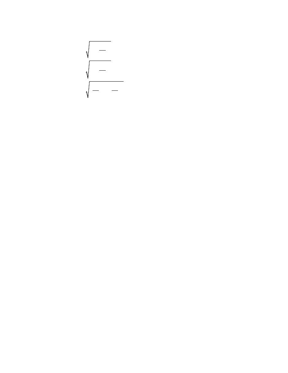
Calculus II

http://tutorial.math.lamar.edu/terms.aspx

where,

( )

if ,

f x

h y

f t

g t





≤ ≤













≤ ≤

















≤ ≤

















Calculus II

http://tutorial.math.lamar.edu/terms.aspx

Surface Area with Parametric Equations

In this final section of looking at calculus applications with parametric equations we will take a
look at determining the surface area of a region obtained by rotating a parametric curve about the
x or y-axis.

We will rotate the parametric curve given by,

( )

f t

g t

≤ ≤

about the x or y-axis. We are going to assume that the curve is traced out exactly once as t
increases from

. At this point there actually isn’t all that much to do. We know that the

surface area can be found by using one of the following two formulas depending on the axis of
rotation (recall the

Surface Area

section of the Applications of Integrals chapter).

rotation about

axis

rotation about

axis

y ds

x ds

−

∫
∫

All that we need is a formula for ds to use and from the previous section we have,

( )

if ,

f t

g t









≤ ≤

















which is exactly what we need.

We will need to be careful with the x or y that is in the original surface area formula. Back when
we first looked at surface area we saw that sometimes we had to substitute for the variable in the
integral and at other times we didn’t. This was dependent upon the ds that we used. In this case
however, we will always have to substitute for the variable. The ds that we use for parametric
equations introduces a dt into the integral and that means that everything needs to be in terms of t.
Therefore, we will need to substitute the appropriate parametric equation for x or y depending on
the axis of rotation.

Let’s take a quick look at an example.

Example 1

Determine the surface area of the solid obtained by rotating the following

parametric curve about the x-axis.

cos

sin

≤ ≤

Solution
We’ll first need the derivatives of the parametric equations.

3cos

sin

3sin

cos

= −

Before plugging into the surface area formula let’s get the ds out of the way.

Calculus II

http://tutorial.math.lamar.edu/terms.aspx

9 cos

sin

9 sin

cos

3 cos sin

cos

sin

3cos sin

Notice that we could drop the absolute value bars since both sine and cosine are positive in this
range of

given.

Now let’s get the surface area and don’t forget to also plug in for the y.

(

)

sin

3cos sin

sin

cos

sin

y ds

u du

θ θ

∫

∫
∫
∫

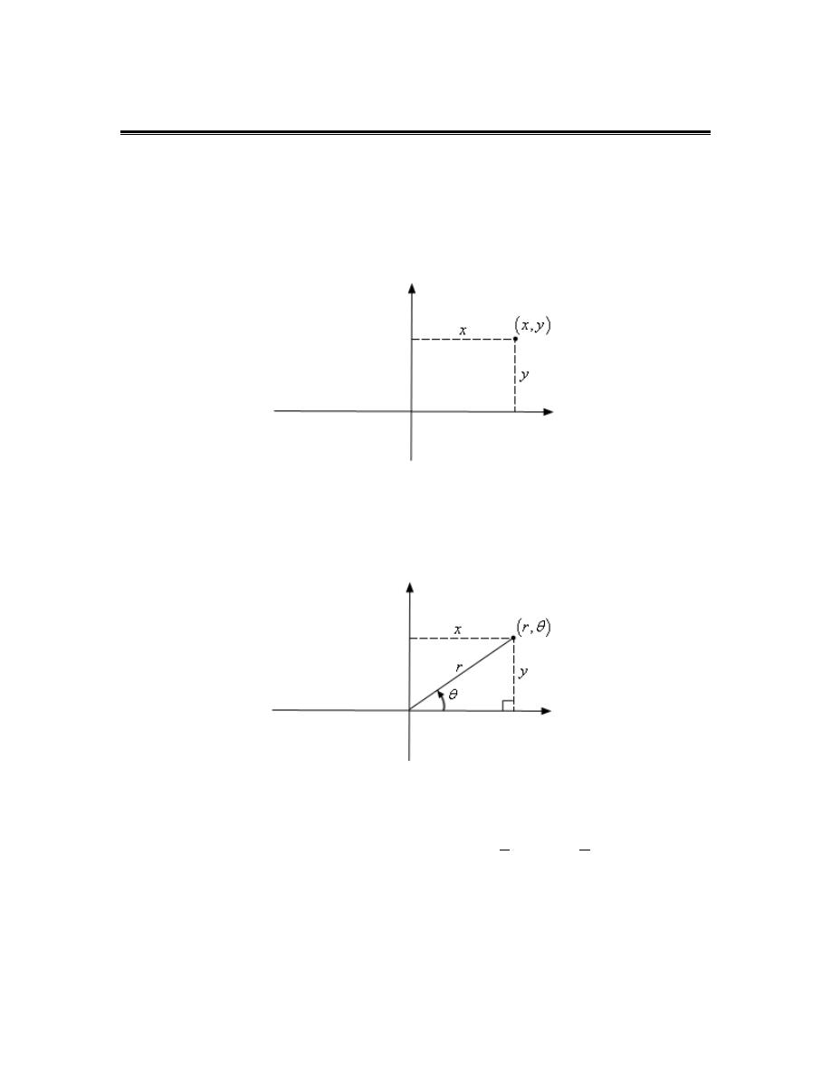
Calculus II

http://tutorial.math.lamar.edu/terms.aspx

Polar Coordinates

Up to this point we’ve dealt exclusively with the Cartesian (or Rectangular, or x-y) coordinate
system. However, as we will see, this is not always the easiest coordinate system to work in. So,
in this section we will start looking at the polar coordinate system.

Coordinate systems are really nothing more than a way to define a point in space. For instance in
the Cartesian coordinate system at point is given the coordinates (x,y) and we use this to define
the point by starting at the origin and then moving x units horizontally followed by y units
vertically. This is shown in the sketch below.

This is not, however, the only way to define a point in two dimensional space. Instead of moving
vertically and horizontally from the origin to get to the point we could instead go straight out of
the origin until we hit the point and then determine the angle this line makes with the positive x-
axis. We could then use the distance of the point from the origin and the amount we needed to
rotate from the positive x-axis as the coordinates of the point. This is shown in the sketch below.

Coordinates in this form are called polar coordinates.

The above discussion may lead one to think that r must be a positive number. However, we also

allow r to be negative. Below is a sketch of the two points

( )

and

(

)

−

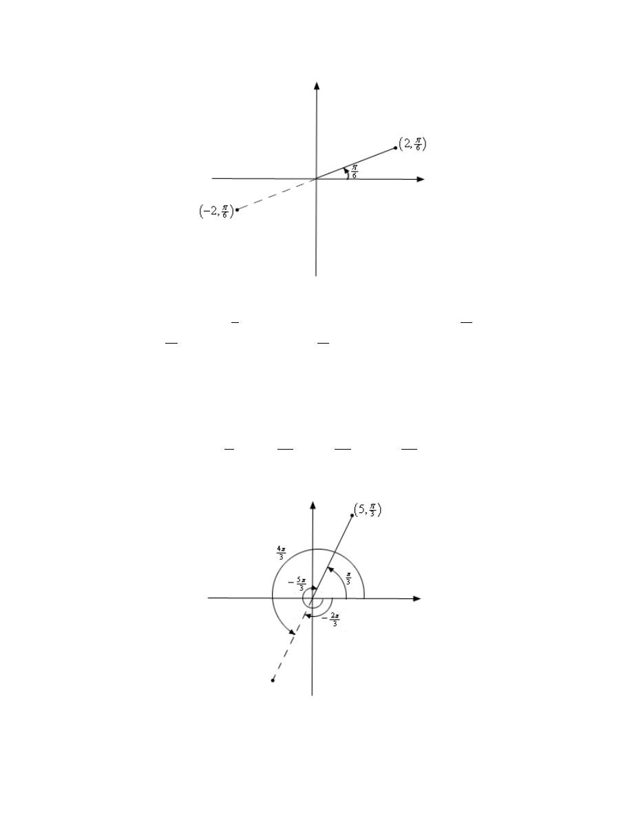
Calculus II

http://tutorial.math.lamar.edu/terms.aspx

From this sketch we can see that if r is positive the point will be in the same quadrant as

. On

the other hand if r is negative the point will end up in the quadrant exactly opposite

. Notice as

well that the coordinates

(

)

−

describe the same point as the coordinates

(

)

do. The

coordinates

(

)

tells us to rotate an angle of

from the positive x-axis, this would put us

on the dashed line in the sketch above, and then move out a distance of 2.

This leads to an important difference between Cartesian coordinates and polar coordinates. In
Cartesian coordinates there is exactly one set of coordinates for any given point. With polar
coordinates this isn’t true. In polar coordinates there is literally an infinite number of coordinates
for a given point. For instance, the following four points are all coordinates for the same point.



 



−

= −

= − −



 





 



Here is a sketch of the angles used in these four sets of coordinates.

In the second coordinate pair we rotated in a clock-wise direction to get to the point. We
shouldn’t forget about rotating in the clock-wise direction. Sometimes it’s what we have to do.

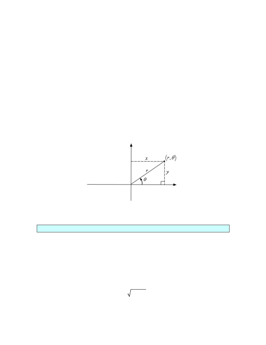
Calculus II

http://tutorial.math.lamar.edu/terms.aspx

The last two coordinate pairs use the fact that if we end up in the opposite quadrant from the point
we can use a negative r to get back to the point and of course there is both a counter clock-wise
and a clock-wise rotation to get to the angle.

These four points only represent the coordinates of the point without rotating around the system
more than once. If we allow the angle to make as many complete rotations about the axis system
as we want then there are an infinite number of coordinates for the same point. In fact the point

( )

can be represented by any of the following coordinate pairs.

(

)

(

)

(

)

where is any integer.

−

Next we should talk about the origin of the coordinate system. In polar coordinates the origin is
often called the pole. Because we aren’t actually moving away from the origin/pole we know
that

. However, we can still rotate around the system by any angle we want and so the

coordinates of the origin/pole are

( )

Now that we’ve got a grasp on polar coordinates we need to think about converting between the
two coordinate systems. Well start out with the following sketch reminding us how both
coordinate systems work.

Note that we’ve got a right triangle above and with that we can get the following equations that
will convert polar coordinates into Cartesian coordinates.

Polar to Cartesian Conversion Formulas

cos

sin

Converting from Cartesian is almost as easy. Let’s first notice the following.

(

) (

)

(

)

cos

sin

cos

sin

cos

sin

This is a very useful formula that we should remember, however we are after an equation for r so
let’s take the square root of both sides. This gives,

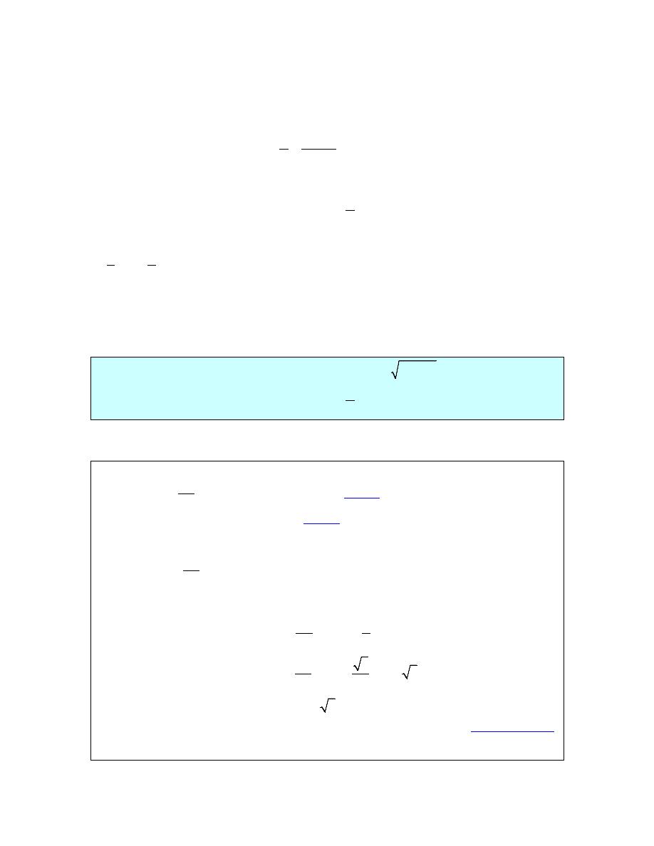
Calculus II

http://tutorial.math.lamar.edu/terms.aspx

Note that technically we should have a plus or minus in front of the root since we know that r can
be either positive or negative. We will run with the convention of positive r here.

Getting an equation for

is almost as simple. We’ll start with,

sin

tan

cos

Taking the inverse tangent of both sides gives,

tan

−

 

 

 

We will need to be careful with this because inverse tangents only return values in the range

− < <

. Recall that there is a second possible angle and that the second angle is given by

θ π

Summarizing then gives the following formulas for converting from Cartesian coordinates to
polar coordinates.

Cartesian to Polar Conversion Formulas

tan

−

 

 

 

Let’s work a quick example.

Example 1

Convert each of the following points into the given coordinate system.

(a)





−









into Cartesian coordinates.

[

Solution

]

(b) (-1,-1) into polar coordinates.

[

Solution

]

Solution

(a) Convert





−









into Cartesian coordinates.

This conversion is easy enough. All we need to do is plug the points into the formulas.

4 cos

4 sin

2 3









= −

= − −

























= −





















So, in Cartesian coordinates this point is

(

)

2, 2 3

−

[

Return to Problems

]

Calculus II

http://tutorial.math.lamar.edu/terms.aspx

(b) Convert (-1,-1) into polar coordinates.

Let’s first get r.

( ) ( )

−

+ −

Now, let’s get

( )

tan

−









−





This is not the correct angle however. This value of

is in the first quadrant and the point we’ve

been given is in the third quadrant. As noted above we can get the correct angle by adding

onto

this. Therefore, the actual angle is,

= + =

So, in polar coordinates the point is

(

)

. Note as well that we could have used the first

that we got by using a negative r. In this case the point could also be written in polar coordinates

(

)

−

[

Return to Problems

]

We can also use the above formulas to convert equations from one coordinate system to the other.

Example 2

Convert each of the following into an equation in the given coordinate system.

(a) Convert

−

= +

into polar coordinates.

[

Solution

]

(b) Convert

8 cos

= −

into Cartesian coordinates.

[

Solution

]

Solution

(a) Convert

−

= +

into polar coordinates.

In this case there really isn’t much to do other than plugging in the formulas for x and y (i.e. the
Cartesian coordinates) in terms of r and

(i.e. the polar coordinates).

(

) (

)

(

)(

)

cos

sin

2 cos

cos

cos sin

−

= +

−

= +

[

Return to Problems

]

(b) Convert

8 cos

= −

into Cartesian coordinates.

This one is a little trickier, but not by much. First notice that we could substitute straight for the
r. However, there is no straight substitution for the cosine that will give us only Cartesian
coordinates. If we had an r on the right along with the cosine then we could do a direct
substitution. So, if an r on the right side would be convenient let’s put one there, just don’t forget
to put one on the left side as well.

8 cos

= −

We can now make some substitutions that will convert this into Cartesian coordinates.

= −

[

Return to Problems

]

Calculus II

http://tutorial.math.lamar.edu/terms.aspx

Before moving on to the next subject let’s do a little more work on the second part of the previous
example.

The equation given in the second part is actually a fairly well known graph; it just isn’t in a form
that most people will quickly recognize. To identify it let’s take the Cartesian coordinate
equation and do a little rearranging.

Now, complete the square on the x portion of the equation.

(

)

So, this was a circle of radius 4 and center (-4,0).

This leads us into the final topic of this section.

Common Polar Coordinate Graphs
Let’s identify a few of the more common graphs in polar coordinates. We’ll also take a look at a
couple of special polar graphs.

Lines
Some lines have fairly simple equations in polar coordinates.

θ β

We can see that this is a line by converting to Cartesian coordinates as follows

(

)

tan

θ β

−

  =

 

 

This is a line that goes through the origin and makes an angle of

with the positive x-

axis. Or, in other words it is a line through the origin with slope of

tan

cos

This is easy enough to convert to Cartesian coordinates to

. So, this is a vertical

line.

sin

Likewise, this converts to

and so is a horizontal line.

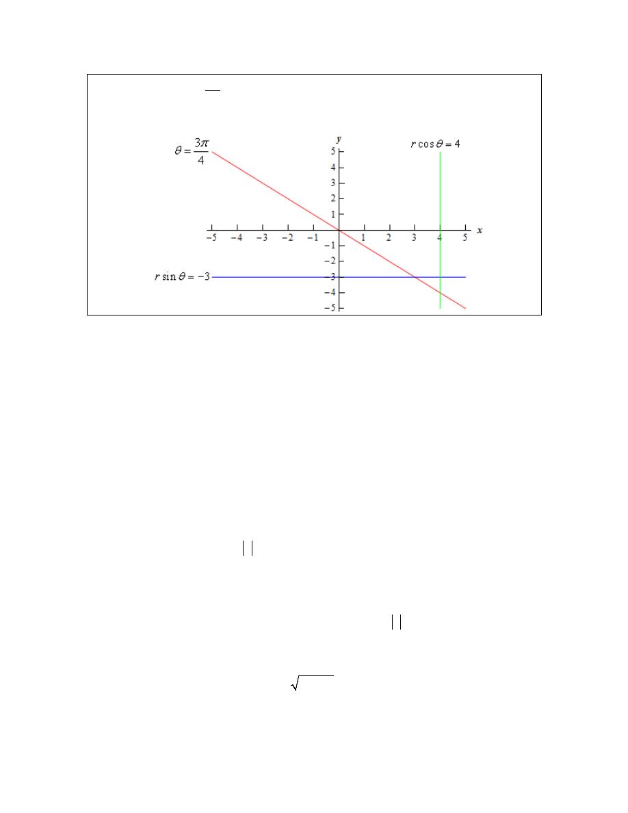
Calculus II

http://tutorial.math.lamar.edu/terms.aspx

Example 3

Graph

cos

and

sin

= −

on the same axis system.

Solution
There really isn’t too much to this one other than doing the graph so here it is.

Circles
Let’s take a look at the equations of circles in polar coordinates.

This equation is saying that no matter what angle we’ve got the distance from the origin
must be a. If you think about it that is exactly the definition of a circle of radius a
centered at the origin.

So, this is a circle of radius a centered at the origin. This is also one of the reasons why
we might want to work in polar coordinates. The equation of a circle centered at the
origin has a very nice equation, unlike the corresponding equation in Cartesian
coordinates.

2 cos

We looked at a specific example of one of these when we were converting equations to
Cartesian coordinates.

This is a circle of radius

and center

( )

, 0

. Note that a might be negative (as it was

in our example above) and so the absolute value bars are required on the radius. They
should not be used however on the center.

2 sin

This is similar to the previous one. It is a circle of radius

and center

( )

0, b

2 cos

2 sin

This is a combination of the previous two and by completing the square twice it can be

shown that this is a circle of radius

and center

( )

a b

. In other words, this is

the general equation of a circle that isn’t centered at the origin.

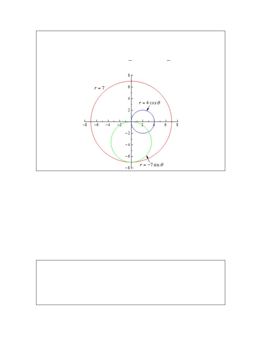
Calculus II

http://tutorial.math.lamar.edu/terms.aspx

Example 4

Graph

4 cos

, and

7 sin

= −

on the same axis system.

Solution
The first one is a circle of radius 7 centered at the origin. The second is a circle of radius 2

centered at (2,0). The third is a circle of radius

centered at





−









. Here is the graph of the

three equations.

Note that it takes a range of

≤ ≤

for a complete graph of

and it only takes a range

θ π

≤ ≤

to graph the other circles given here.

Cardioids and Limacons
These can be broken up into the following three cases.

1. Cardioids :

cos

= ±

and

sin

= ±

These have a graph that is vaguely heart shaped and always contain the origin.

2. Limacons with an inner loop :

cos

a b

= ±

and

sin

a b

= ±

with

These will have an inner loop and will always contain the origin.

3. Limacons without an inner loop :

cos

a b

= ±

and

sin

a b

= ±

with

These do not have an inner loop and do not contain the origin.

Example 5

Graph

5 5sin

= −

7 6 cos

= −

, and

2 4 cos

= +

Solution
These will all graph out once in the range

≤ ≤

. Here is a table of values for each

followed by graphs of each.

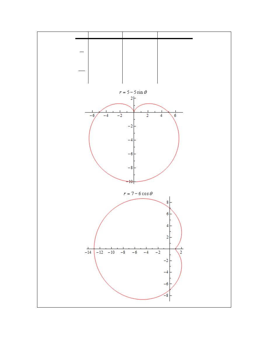
Calculus II

http://tutorial.math.lamar.edu/terms.aspx

5 5sin

= −

7 6 cos

= −

2 4 cos

= +

-2

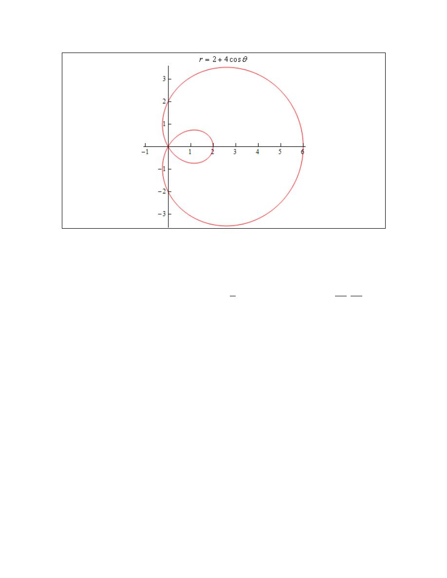
Calculus II

http://tutorial.math.lamar.edu/terms.aspx

There is one final thing that we need to do in this section. In the third graph in the previous
example we had an inner loop. We will, on occasion, need to know the value of

for which the

graph will pass through the origin. To find these all we need to do is set the equation equal to
zero and solve as follows,

2 4 cos

cos

π π

= +

⇒

= −

⇒

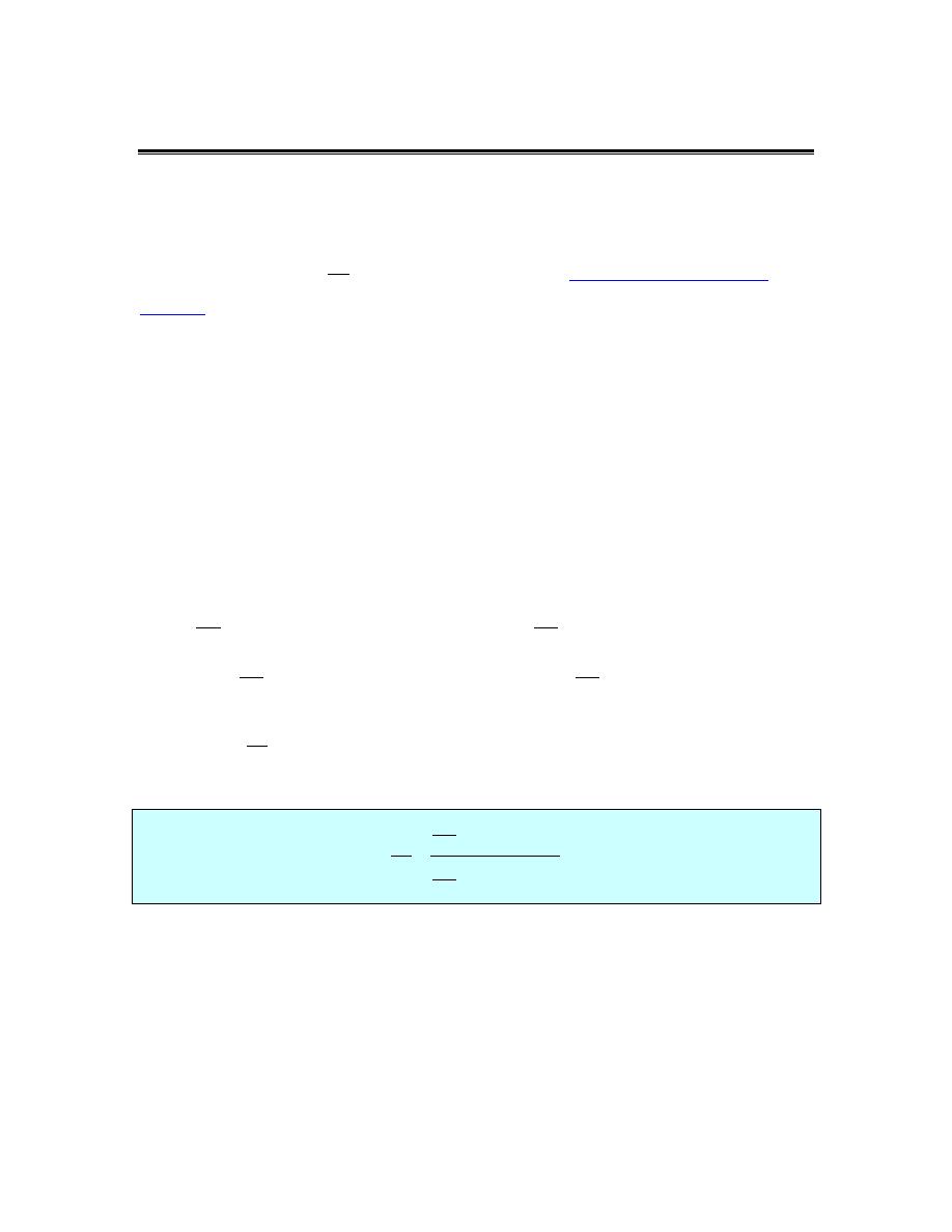
Calculus II

http://tutorial.math.lamar.edu/terms.aspx

Tangents with Polar Coordinates

We now need to discuss some calculus topics in terms of polar coordinates.

We will start with finding tangent lines to polar curves. In this case we are going to assume that

the equation is in the form

( )

. With the equation in this form we can actually use the

equation for the derivative

we derived when we looked at

tangent lines with parametric

equations

. To do this however requires us to come up with a set of parametric equations to

represent the curve. This is actually pretty easy to do.

From our work in the previous section we have the following set of conversion equations for
going from polar coordinates to Cartesian coordinates.

cos

sin

Now, we’ll use the fact that we’re assuming that the equation is in the form

( )

Substituting this into these equations gives the following set of parametric equations (with

the parameter) for the curve.

( )

cos

sin

Now, we will need the following derivatives.

( )

cos

sin

cos

sin

cos

′

−

The derivative

is then,

Derivative with Polar Coordinates

sin

cos

sin

−

Note that rather than trying to remember this formula it would probably be easier to remember
how we derived it and just remember the formula for parametric equations.

Let’s work a quick example with this.

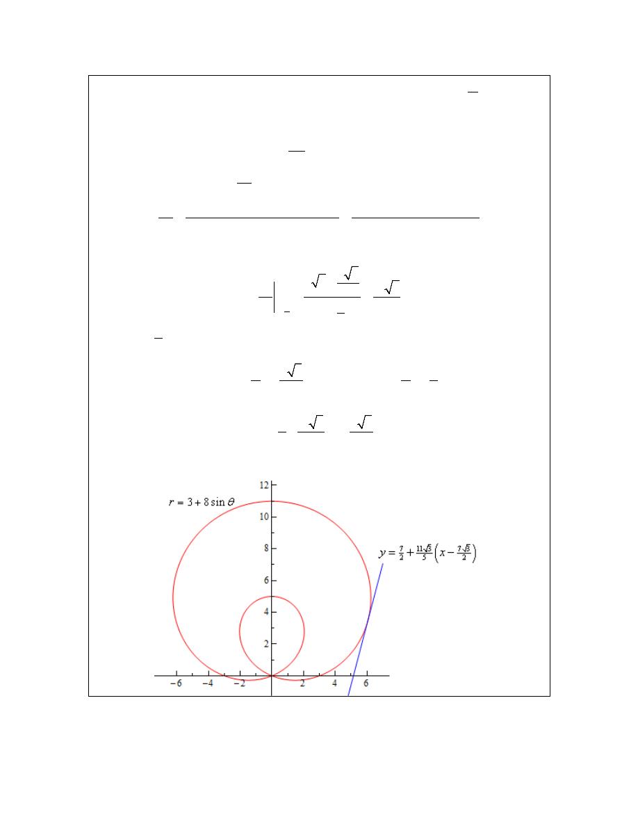
Calculus II

http://tutorial.math.lamar.edu/terms.aspx

Example 1

Determine the equation of the tangent line to

3 8sin

= +

Solution
We’ll first need the following derivative.

8 cos

The formula for the derivative

becomes,

(

)

(

)

8 cos sin

3 8sin

cos

16 cos sin

3cos

8 cos

3 8sin

sin

8 cos

3sin

8sin

+ +

− +

−

The slope of the tangent line is,

3 3

4 3

11 3

θ =

−

Now, at

θ =

we have

. We’ll need to get the corresponding x-y coordinates so we can

get the tangent line.

7 3

7 cos

7 sin

 

 

 

The tangent line is then,

11 3

7 3





= +

−













For the sake of completeness here is a graph of the curve and the tangent line.

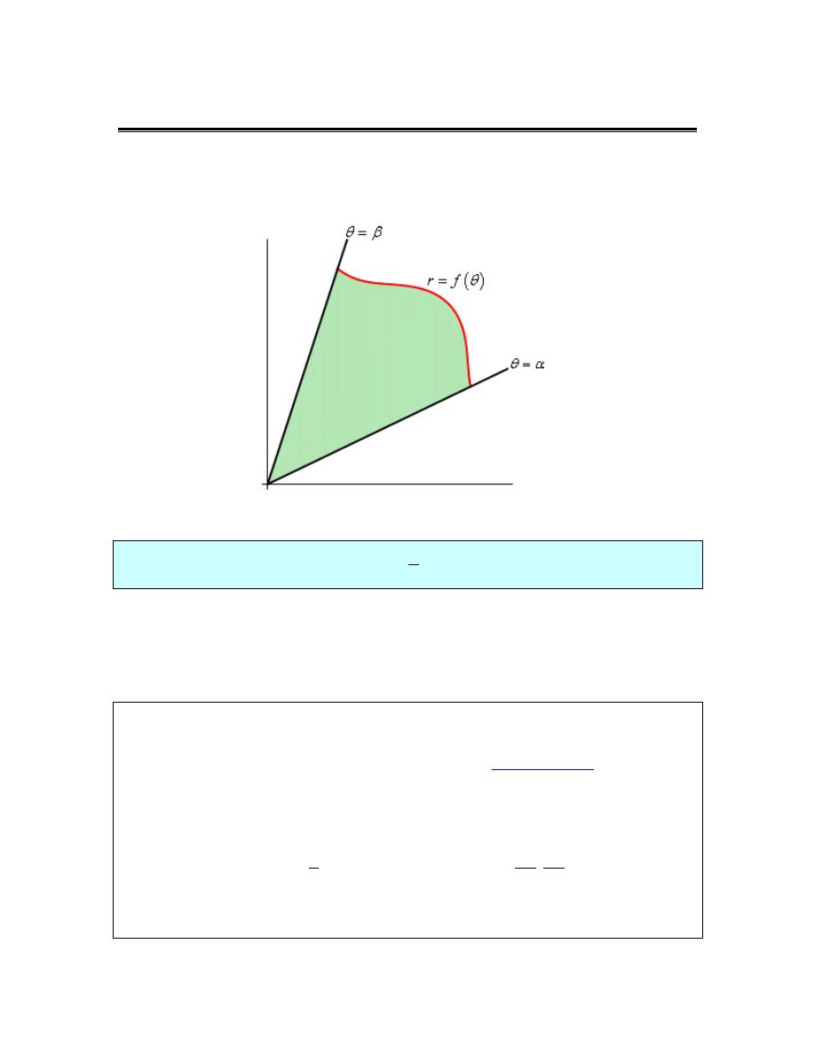
Calculus II

http://tutorial.math.lamar.edu/terms.aspx

Area with Polar Coordinates

In this section we are going to look at areas enclosed by polar curves. Note as well that we said
“enclosed by” instead of “under” as we typically have in these problems. These problems work a
little differently in polar coordinates. Here is a sketch of what the area that we’ll be finding in
this section looks like.

We’ll be looking for the shaded area in the sketch above. The formula for finding this area is,

r d

= ⌠



⌡

Notice that we use r in the integral instead of

( )

so make sure and substitute accordingly

when doing the integral.

Let’s take a look at an example.

Example 1

Determine the area of the inner loop of

2 4 cos

= +

Solution
We graphed this function back when we first started looking at

polar coordinates

. For this

problem we’ll also need to know the values of

where the curve goes through the origin. We

can get these by setting the equation equal to zero and solving.

2 4 cos

cos

π π

= +

= −

⇒

Here is the sketch of this curve with the inner loop shaded in.

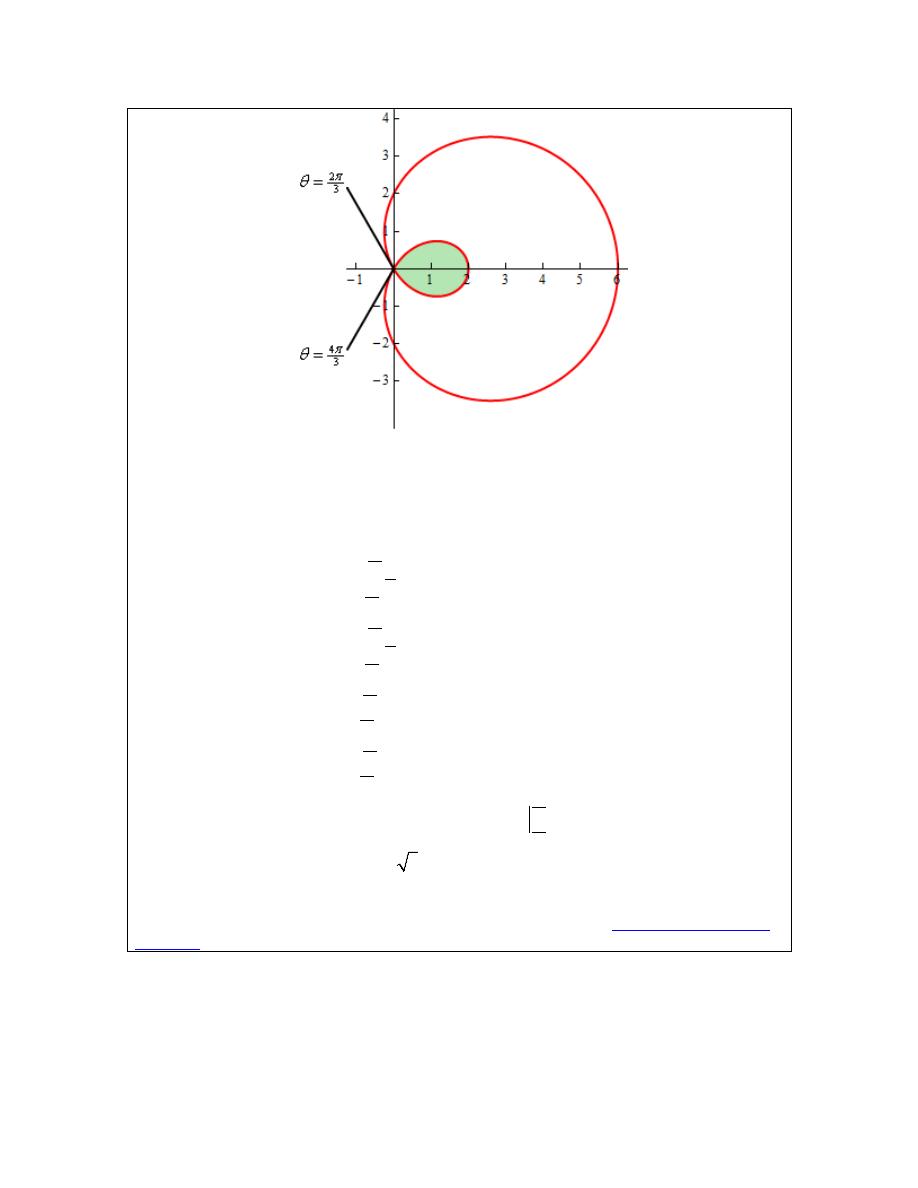
Calculus II

http://tutorial.math.lamar.edu/terms.aspx

Can you see why we needed to know the values of

where the curve goes through the origin?

These points define where the inner loop starts and ends and hence are also the limits of
integration in the formula.

So, the area is then,

(

)

(

)

( )

(

)

( )

(

)

2 4 cos

4 16 cos

16 cos

2 8 cos

4 1 cos 2

6 8 cos

4 cos 2

8sin

2 sin 2

6 3

2.174

θ θ

−

⌠



⌡

⌠



⌡

∫

You did follow the work done in this integral didn’t you? You’ll run into quite a few integrals of
trig functions in this section so if you need to you should go back to the

Integrals Involving Trig

Functions

sections and do a quick review.

So, that’s how we determine areas that are enclosed by a single curve, but what about situations
like the following sketch were we want to find the area between two curves.

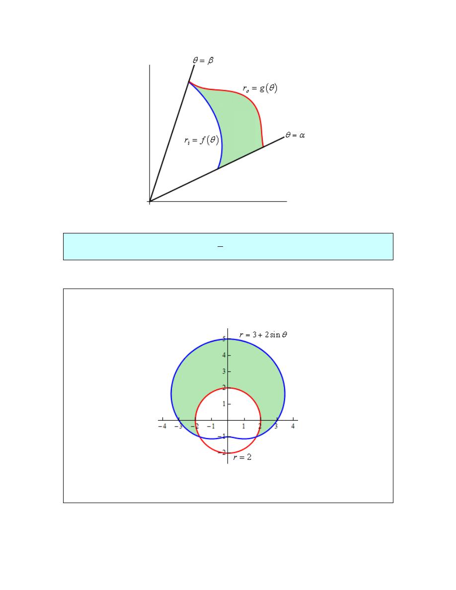
Calculus II

http://tutorial.math.lamar.edu/terms.aspx

In this case we can use the above formula to find the area enclosed by both and then the actual
area is the difference between the two. The formula for this is,

(

)

−

⌠



⌡

Let’s take a look at an example of this.

Example 2

Determine the area that lies inside

3 2 sin

= +

and outside

Solution
Here is a sketch of the region that we are after.

To determine this area we’ll need to know the values of

for which the two curves intersect. We

can determine these points by setting the two equations and solving.

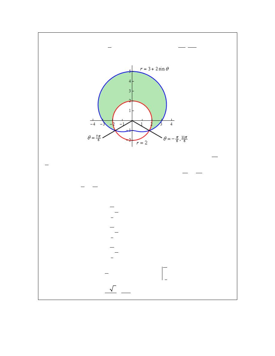
Calculus II

http://tutorial.math.lamar.edu/terms.aspx

3 2 sin

sin

= −

⇒

Here is a sketch of the figure with these angles added.

Note as well here that we also acknowledged that another representation for the angle

−

. This is important for this problem. In order to use the formula above the area must be

enclosed as we increase from the smaller to larger angle. So, if we use

we will not

enclose the shaded area, instead we will enclose the bottom most of the three regions. However if
we use the angles

−

we will enclose the area that we’re after.

So, the area is then,

(

) ( )

(

)

(

)

( )

(

)

( )

(

)

3 2 sin

5 12 sin

4 sin

7 12 sin

2 cos 2

12 cos

sin 2

11 3

24.187

θ θ

−

⌠



⌡

⌠



⌡

⌠



⌡

Let’s work a slight modification of the previous example.

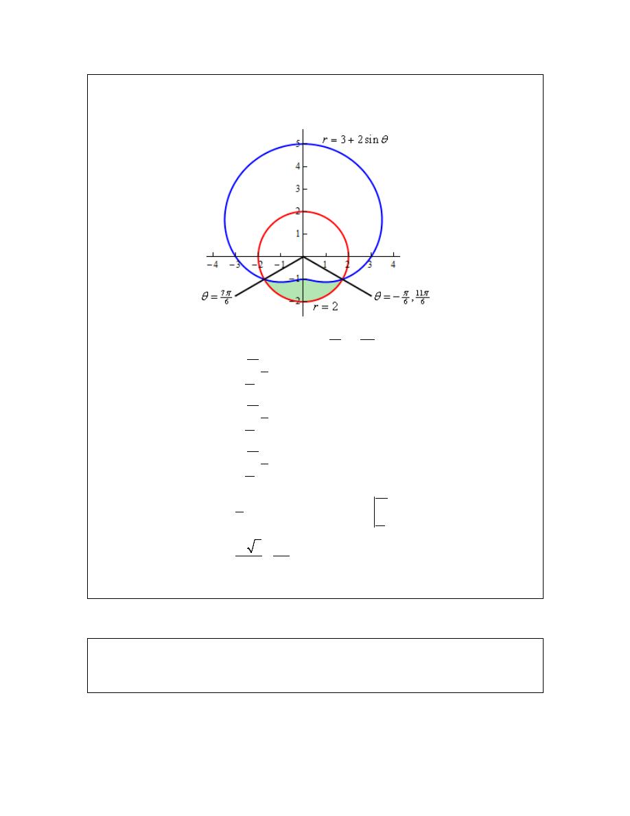
Calculus II

http://tutorial.math.lamar.edu/terms.aspx

Example 3

Determine the area of the region outside

3 2 sin

= +

and inside

Solution
This time we’re looking for the following region.

So, this is the region that we get by using the limits

. The area for this region is,

( ) (

)

(

)

(

)

( )

(

)

( )

(

)

3 2 sin

5 12 sin

4 sin

7 12 sin

2 cos 2

12 cos

sin 2

11 3

2.196

θ θ

− +

− −

−

− −

−

⌠



⌡

⌠



⌡

⌠



⌡

Notice that for this area the “outer” and “inner” function were opposite!

Let’s do one final modification of this example.

Example 4

Determine the area that is inside both

3 2 sin

= +

and

Solution
Here is the sketch for this example.

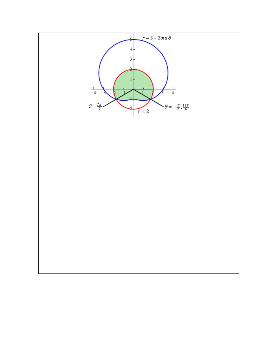
Calculus II

http://tutorial.math.lamar.edu/terms.aspx

We are not going to be able to do this problem in the same fashion that we did the previous two.
There is no set of limits that will allow us to enclose this area as we increase from one to the
other. Remember that as we increase

the area we’re after must be enclosed. However, the

only two ranges for

that we can work with enclose the area from the previous two examples

and not this region.

In this case however, that is not a major problem. There are two ways to do get the area in this
problem. We’ll take a look at both of them.

Solution 1
In this case let’s notice that the circle is divided up into two portions and we’re after the upper
portion. Also notice that we found the area of the lower portion in Example 3. Therefore, the
area is,

( )

Area

Area of Circle Area from Example 3

2.196

10.370

−

Solution 2
In this case we do pretty much the same thing except this time we’ll think of the area as the other
portion of the limacon than the portion that we were dealing with in Example 2. We’ll also need
to actually compute the area of the limacon in this case.

So, the area using this approach is then,

Calculus II

http://tutorial.math.lamar.edu/terms.aspx

(

)

(

)

( )

(

)

( )

(

)

Area

Area of Limacon

Area from Example 2

3 2 sin

24.187

9 12 sin

4 sin

24.187

11 12 sin

2 cos 2

24.187

12 cos

sin 2

24.187

10.370

θ θ

−

⌠



⌡

⌠



⌡

⌠



⌡

A slightly longer approach, but sometimes we are forced to take this longer approach.

As this last example has shown we will not be able to get all areas in polar coordinates straight
from an integral.

Calculus II

http://tutorial.math.lamar.edu/terms.aspx

Arc Length with Polar Coordinates

We now need to move into the Calculus II applications of integrals and how we do them in terms
of polar coordinates. In this section we’ll look at the arc length of the curve given by,

( )

α θ β

≤ ≤

where we also assume that the curve is traced out exactly once. Just as we did with the

tangent

lines in polar coordinates

we’ll first write the curve in terms of a set of parametric equations,

( )

cos

sin

cos

sin

and we can now use the parametric formula for finding the arc length.

We’ll need the following derivatives for these computations.

( )

cos

sin

cos

sin

cos

′

−

We’ll need the following for our ds.

(

) (

)

cos

sin

cos

cos sin

sin

cos sin

cos

sin

cos

sin

















−





































−





































+ 







The arc length formula for polar coordinates is then,

∫

where,





+ 







Let’s work a quick example of this.

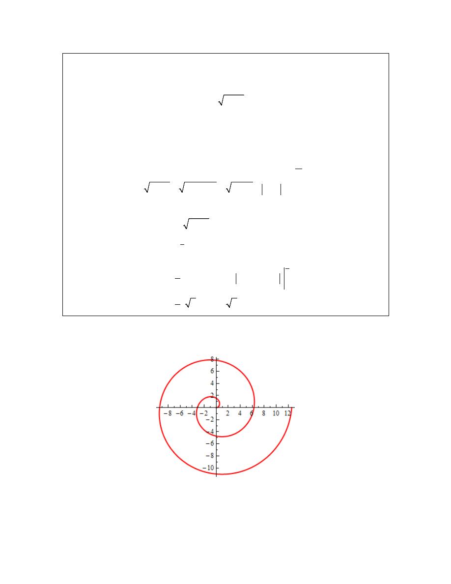
Calculus II

http://tutorial.math.lamar.edu/terms.aspx

Example 1

Determine the length of

≤ ≤

Solution
Okay, let’s just jump straight into the formula since this is a fairly simple function.

∫

We’ll need to use a trig substitution here.

tan

sec

x dx

tan

sec

+ =

The arc length is then,

(

)

(

)

(

)

sec

sec tan

ln sec

tan

ln 1

x dx

∫
∫

Just as an aside before we leave this chapter. The polar equation

is the equation of a

spiral. Here is a quick sketch of

for

≤ ≤

Calculus II

http://tutorial.math.lamar.edu/terms.aspx

Surface Area with Polar Coordinates

We will be looking at surface area in polar coordinates in this section. Note however that all
we’re going to do is give the formulas for the surface area since most of these integrals tend to be
fairly difficult.

We want to find the surface area of the region found by rotating,

( )

α θ β

≤ ≤

about the x or y-axis.

As we did in the

tangent

and

arc length

sections we’ll write the curve in terms of a set of

parametric equations.

( )

cos

sin

cos

sin

If we now use the parametric formula for finding the surface area we’ll get,

rotation about

axis

rotation about

axis

y ds

x ds

−

∫
∫

where,

( )

α θ β





≤ ≤









Note that because we will pick up a

from the ds we’ll need to substitute one of the parametric

equations in for x or y depending on the axis of rotation. This will often mean that the integrals
will be somewhat unpleasant.

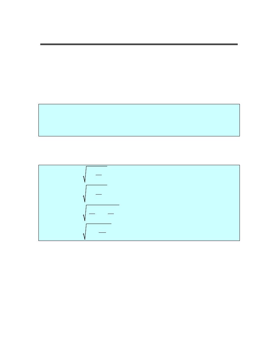
Calculus II

http://tutorial.math.lamar.edu/terms.aspx

Arc Length and Surface Area Revisited

We won’t be working any examples in this section.  This section is here solely for the purpose of
summarizing up all the arc length and surface area problems.

Over the course of the last two chapters the topic of arc length and surface area has arisen many
times and each time we got a new formula out of the mix. Students often get a little overwhelmed
with all the formulas.

However, there really aren’t as many formulas as it might seem at first glance.  There is exactly
one arc length formula and exactly two surface area formulas. These are,

rotation about

axis

rotation about

axis

y ds

x ds

−

∫
∫
∫

The problems arise because we have quite a few ds’s that we can use. Again students often have
trouble deciding which one to use. The examples/problems usually suggest the correct one to use
however. Here is a complete listing of all the ds’s that we’ve seen and when they are used.

( )

if ,

f x

h y

f t

g t

α θ β





≤ ≤













≤ ≤

















≤ ≤





















≤ ≤









Depending on the form of the function we can quickly tell which ds to use.

There is only one other thing to worry about in terms of the surface area formula. The ds will
introduce a new differential to the integral. Before integrating make sure all the variables are in
terms of this new differential. For example if we have parametric equations we’ll use the third ds
and then we’ll need to make sure and substitute for the x or y depending on which axis we rotate
about to get everything in terms of t.

Likewise, if we have a function in the form

( )

h y

then we’ll use the second ds and if the

rotation is about the y-axis we’ll need to substitute for the x in the integral. On the other hand if
we rotate about the x-axis we won’t need to do a substitution for the y.

Calculus II

http://tutorial.math.lamar.edu/terms.aspx

Keep these rules in mind and you’ll always be able to determine which formula to use and how to
correctly do the integral.

Calculus II

http://tutorial.math.lamar.edu/terms.aspx