
CALCULUS II
Solutions to Practice Problems
Integration Techniques
Paul Dawkins

Calculus II
© 2007 Paul Dawkins
i
http://tutorial.math.lamar.edu/terms.aspx
Table of Contents
Preface ............................................................................................................................................ 1
Integration Techniques ................................................................................................................. 1
Integration by Parts .................................................................................................................................... 1
Integrals Involving Trig Functions ............................................................................................................11
Trig Substitutions ......................................................................................................................................23
Partial Fractions ........................................................................................................................................46
Integrals Involving Roots ..........................................................................................................................56
Integrals Involving Quadratics ..................................................................................................................60
Integration Strategy ...................................................................................................................................65
Improper Integrals .....................................................................................................................................65
Comparison Test for Improper Integrals ...................................................................................................81
Approximating Definite Integrals .............................................................................................................93
Preface
Here are the solutions to the practice problems for my Calculus II notes. Some solutions will have more
or less detail than other solutions. As the difficulty level of the problems increases less detail will go into
the basics of the solution under the assumption that if you’ve reached the level of working the harder
problems then you will probably already understand the basics fairly well and won’t need all the
explanation.
This document was written with presentation on the web in mind. On the web most solutions are broken
down into steps and many of the steps have hints. Each hint on the web is given as a popup however in
this document they are listed prior to each step. Also, on the web each step can be viewed individually by
clicking on links while in this document they are all showing. Also, there are liable to be some formatting
parts in this document intended for help in generating the web pages that haven’t been removed here.
These issues may make the solutions a little difficult to follow at times, but they should still be readable.
Integration Techniques
Integration by Parts
1. Evaluate
(
)
4 cos 2 3
x
x dx
−
∫
.
Hint : Remember that we want to pick u and dv so that upon computing du and v and plugging everything
into the Integration by Parts formula the new integral is one that we can do.
Step 1

Calculus II
© 2007 Paul Dawkins
2
http://tutorial.math.lamar.edu/terms.aspx
The first step here is to pick u and dv. We want to choose u and dv so that when we compute du and v
and plugging everything into the Integration by Parts formula the new integral we get is one that we can
do.
With that in mind it looks like the following choices for u and dv should work for us.
(
)
4
cos 2 3
u
x
dv
x dx
=
=
−
Step 2
Next we need to compute du (by differentiating u) and v (by integrating dv).
(
)
(
)
1
3
4
4
cos 2 3
sin 2 3
u
x
du
dx
dv
x dx
v
x
=
→
=
=
−
→
= −
−
Step 3
Plugging u, du, v and dv into the Integration by Parts formula gives,
(
)
( )
(
)
(
)
(
)
(
)
(
)
1
4
3
3
4
4
3
3
4 cos 2 3
4
sin 2 3
sin 2 3
sin 2 3
sin 2 3
x
x dx
x
x
x dx
x
x
x dx
−
=
−
−
− −
−
= −
−
+
−
∫
∫
∫
Step 4
Okay, the new integral we get is easily doable and so all we need to do to finish this problem out is do the
integral.
(
)
(
)
(
)
4
4
3
9
4 cos 2 3
sin 2 3
cos 2 3
x
x dx
x
x
x
c
−
= −
−
+
−
+
∫
2. Evaluate
(
)
1
3
0
6
2 5
x
x
dx
+
∫
e
.
Hint : Remember that we want to pick u and dv so that upon computing du and v and plugging everything
into the Integration by Parts formula the new integral is one that we can do.
Also, don’t forget that the limits on the integral won’t have any effect on the choices of u and dv.
Step 1
The first step here is to pick u and dv. We want to choose u and dv so that when we compute du and v
and plugging everything into the Integration by Parts formula the new integral we get is one that we can
do.
With that in mind it looks like the following choices for u and dv should work for us.
1
3
2 5
x
u
x
dv
dx
= +
= e
Step 2

Calculus II
© 2007 Paul Dawkins
3
http://tutorial.math.lamar.edu/terms.aspx
Next we need to compute du (by differentiating u) and v (by integrating dv).
1
1
3
3
2 5
5
3
x
x
u
x
du
dx
dv
dx
v
= +
→
=
=
→
=
e
e
Step 3
We can deal with the limits as we do the integral or we can just do the indefinite integral and then take
care of the limits in the last step. We will be using the later way of dealing with the limits for this
problem.
So, plugging u, du, v and dv into the Integration by Parts formula gives,
(
)
(
)
( ) ( )
(
)
1
1
1
1
1
3
3
3
3
3
2 5
2 5
3
5 3
3
2 5
15
x
x
x
x
x
x
x
dx
x
dx
+
=
+
−
=
+
−
∫
∫
∫
e
e
e
e
e
Step 4
Okay, the new integral we get is easily doable so let’s evaluate it to get,
(
)
(
)
1
1
1
1
1
3
3
3
3
3
2 5
3
2 5
45
15
39
x
x
x
x
x
x
x
c
x
c
+
=
+
−
+ =
−
+
∫
e
e
e
e
e
Step 5
The final step is then to take care of the limits.
(
)
(
)
1
1
1
3
3
3
0
0
2
6
6
2 5
15
39
39 51
415.8419
x
x
x
x
dx
x
+
=
−
= − −
= −
∫
e
e
e
e
Do not get excited about the fact that the lower limit is larger than the upper limit. This can happen on
occasion and in no way affects how the integral is evaluated.
3. Evaluate
(
)
( )
2
3
sin 2
t
t
t dt
+
∫
.
Hint : Remember that we want to pick u and dv so that upon computing du and v and plugging everything
into the Integration by Parts formula the new integral is one that we can do (or at least will be easier to
deal with).
Step 1
The first step here is to pick u and dv. We want to choose u and dv so that when we compute du and v
and plugging everything into the Integration by Parts formula the new integral we get is one that we can
do, or will at least be an integral that will be easier to deal with.
With that in mind it looks like the following choices for u and dv should work for us.
( )
2
3
sin 2
u
t
t
dv
t dt
= +
=
Calculus II
© 2007 Paul Dawkins
4
http://tutorial.math.lamar.edu/terms.aspx
Step 2
Next we need to compute du (by differentiating u) and v (by integrating dv).
(
)
( )
( )
2
1
2
3
3 2
sin 2
cos 2
u
t
t
du
t dt
dv
t dt
v
t
= +
→
= +
=
→
= −
Step 3
Plugging u, du, v and dv into the Integration by Parts formula gives,
(
)
( )
(
)
( )
(
) ( )
2
2
1
1
2
2
3
sin 2
3
cos 2
3 2 cos 2
t
t
t dt
t
t
t
t
t dt
+
= −
+
+
+
∫
∫
Step 4
Now, the new integral is still not one that we can do with only Calculus I techniques. However, it is one
that we can do another integration by parts on and because the power on the t’s have gone down by one
we are heading in the right direction.
So, here are the choices for u and dv for the new integral.
( )
( )
1
2
3 2
2
cos 2
sin 2
u
t
du
dt
dv
t dt
v
t
= +
→
=
=
→
=
Step 5
Okay, all we need to do now is plug these new choices of u and dv into the new integral we got in Step 3
and finish the problem out.
(
)
( )
(
)
( )
(
) ( )
( )
(
)
( )
(
) ( )
( )
(
)
( ) (
) ( )
( )
2
2
1
1
1
2
2
2
2
1
1
1
1
2
2
2
2
2
1
1
1
2
4
4
3
sin 2
3
cos 2
3 2 sin 2
sin 2
3
cos 2
3 2 sin 2
cos 2
3
cos 2
3 2 sin 2
cos 2
t
t
t dt
t
t
t
t
t
t dt
t
t
t
t
t
t
c
t
t
t
t
t
t
c
+
= −
+
+
+
−
= −
+
+
+
+
+
= −
+
+
+
+
+
∫
∫
4. Evaluate
( )
1
8
6 tan
w
dw
−
∫
.
Hint : Be careful with your choices of u and dv here. If you think about it there is really only one way
that the choice can be made here and have the problem be workable.
Step 1
The first step here is to pick u and dv.
Note that if we choose the inverse tangent for dv the only way to get v is to integrate dv and so we would
need to know the answer to get the answer and so that won’t work for us. Therefore, the only real choice
for the inverse tangent is to let it be u.
So, here are our choices for u and dv.

Calculus II
© 2007 Paul Dawkins
5
http://tutorial.math.lamar.edu/terms.aspx
( )
1
8
6 tan
w
u
dv
dw
−
=
=
Don’t forget the dw! The differential dw still needs to be put into the dv even though there is nothing else
left in the integral.
Step 2
Next we need to compute du (by differentiating u) and v (by integrating dv).
( )
( )
2
2
2
8
8
1
8
2
64
8
6 tan
6
6
1
1
w
w
w
w
w
u
du
dw
dw
dv
dw
v
w
−
−
−
=
→
=
=
+
+
=
→
=
Step 3
In order to complete this problem we’ll need to do some rewrite on du as follows,
2
48
64
du
dw
w
−
=
+
Plugging u, du, v and dv into the Integration by Parts formula gives,
( )
( )
1
1
8
8
2
6 tan
6 tan
48
64
w
w
w
dw
w
dw
w
−
−
=
+
+
⌠
⌡
∫
Step 4
Okay, the new integral we get is easily doable (with the substitution
2
64
u
w
=
+
) and so all we need to
do to finish this problem out is do the integral.
( )
( )
1
1
2
8
8
6 tan
6 tan
24 ln
64
w
w
dw
w
w
c
−
−
=
+
+
+
∫
5. Evaluate
( )
2
1
4
cos
z
z dz
∫
e
.
Hint : This is one of the few integration by parts problems where either function can go on u and dv. Be
careful however to not get locked into an endless cycle of integration by parts.
Step 1
The first step here is to pick u and dv.
In this case we can put the exponential in either the u or the dv and the cosine in the other. It is one of the
few problems where the choice doesn’t really matter.
For this problem well use the following choices for u and dv.
( )
2
1
4
cos
z
u
z
dv
dz
=
= e

Calculus II
© 2007 Paul Dawkins
6
http://tutorial.math.lamar.edu/terms.aspx
Step 2
Next we need to compute du (by differentiating u) and v (by integrating dv).
( )
( )
1
1
1
4
4
4
2
2
1
2
cos
sin
z
z
u
z
du
z dz
dv
dz
v
=
→
= −
=
→
=
e
e
Step 3
Plugging u, du, v and dv into the Integration by Parts formula gives,
( )
( )
( )
2
2
2
1
1
1
1
1
4
2
4
8
4
cos
cos
sin
z
z
z
z dz
z
z dz
=
+
∫
∫
e
e
e
Step 4
We’ll now need to do integration by parts again and to do this we’ll use the following choices.
( )
( )
1
1
1
4
4
4
2
2
1
2
sin
cos
z
z
u
z
du
z dz
dv
dz
v
=
→
=
=
→
=
e
e
Step 5
Plugging these into the integral from Step 3 gives,
( )
( )
( )
( )
( )
( )
( )
2
2
2
2
1
1
1
1
1
1
1
1
4
2
4
8
2
4
8
4
2
2
2
1
1
1
1
1
1
2
4
16
4
64
4
cos
cos
sin
cos
cos
sin
cos
z
z
z
z
z
z
z
z dz
z
z
z dz
z
z
z dz
=
+
−
=
+
−
∫
∫
∫
e
e
e
e
e
e
e
Step 6
To finish this problem all we need to do is some basic algebraic manipulation to get the identical integrals
on the same side of the equal sign.
( )
( )
( )
( )
( )
( )
( )
( )
( )
( )
( )
2
2
2
2
1
1
1
1
1
1
1
4
2
4
16
4
64
4
2
2
2
2
1
1
1
1
1
1
1
4
64
4
2
4
16
4
2
2
2
65
1
1
1
1
1
64
4
2
4
16
4
cos
cos
sin
cos
cos
cos
cos
sin
cos
cos
sin
z
z
z
z
z
z
z
z
z
z
z
z dz
z
z
z dz
z dz
z dz
z
z
z dz
z
z
=
+
−
+
=
+
=
+
∫
∫
∫
∫
∫
e
e
e
e
e
e
e
e
e
e
e
Finally, all we need to do is move the coefficient on the integral over to the right side.
( )
( )
( )
2
2
2
32
1
1
4
1
4
65
4
65
4
cos
cos
sin
z
z
z
z dz
z
z
c
=
+
+
∫
e
e
e
6. Evaluate
( )
2
0
cos 4
x
x dx
π
∫
.
Hint : Remember that we want to pick u and dv so that upon computing du and v and plugging everything
into the Integration by Parts formula the new integral is one that we can do (or at least will be easier to
deal with).

Calculus II
© 2007 Paul Dawkins
7
http://tutorial.math.lamar.edu/terms.aspx
Also, don’t forget that the limits on the integral won’t have any effect on the choices of u and dv.
Step 1
The first step here is to pick u and dv. We want to choose u and dv so that when we compute du and v
and plugging everything into the Integration by Parts formula the new integral we get is one that we can
do, or will at least be an integral that will be easier to deal with.
With that in mind it looks like the following choices for u and dv should work for us.
( )
2
cos 4
u
x
dv
x dx
=
=
Step 2
Next we need to compute du (by differentiating u) and v (by integrating dv).
( )
( )
2
1
4
2
cos 4
sin 4
u
x
du
x dx
dv
x dx
v
x
=
→
=
=
→
=
Step 3
We can deal with the limits as we do the integral or we can just do the indefinite integral and then take
care of the limits in the last step. We will be using the later way of dealing with the limits for this
problem.
So, plugging u, du, v and dv into the Integration by Parts formula gives,
( )
( )
( )
2
2
1
1
4
2
cos 4
sin 4
sin 4
x
x dx
x
x
x
x dx
=
−
∫
∫
Step 4
Now, the new integral is still not one that we can do with only Calculus I techniques. However, it is one
that we can do another integration by parts on and because the power on the x’s have gone down by one
we are heading in the right direction.
So, here are the choices for u and dv for the new integral.
( )
( )
1
4
sin 4
cos 4
u
x
du
dx
dv
x dx
v
x
=
→
=
=
→
= −
Step 5
Okay, all we need to do now is plug these new choices of u and dv into the new integral we got in Step 3
and evaluate the integral.
( )
( )
( )
( )
( )
( )
( )
( )
( )
( )
2
2
1
1
1
1
4
2
4
4
2
1
1
1
1
4
2
4
16
2
1
1
1
4
8
32
cos 4
sin 4
cos 4
cos 4
sin 4
cos 4
sin 4
sin 4
cos 4
sin 4
x
x dx
x
x
x
x
x dx
x
x
x
x
x
c
x
x
x
x
x
c
=
− −
+
=
− −
+
+
=
+
−
+
∫
∫

Calculus II
© 2007 Paul Dawkins
8
http://tutorial.math.lamar.edu/terms.aspx
Step 6
The final step is then to take care of the limits.
( )
( )
( )
( )
(
)
2
2
1
1
1
1
4
8
32
8
0
0
cos 4
sin 4
cos 4
sin 4
x
x dx
x
x
x
x
x
π
π
π
=
+
−
=
∫
7. Evaluate
( )
7
4
sin 2
t
t
dt
∫
.
Hint : Be very careful with your choices of u and dv for this problem. It looks a lot like previous practice
problems but it isn’t!
Step 1
The first step here is to pick u and dv and, in this case, we’ll need to be careful how we chose them.
If we follow the model of many of the examples/practice problems to this point it is tempting to let u be
7
t
and to let dv be
( )
4
sin 2t
.
However, this will lead to some real problems. To compute v we’d have to integrate the sine and because
of the
4
t
in the argument this is not possible. In order to integrate the sine we would have to have a
3
t
in
the integrand as well in order to a substitution as shown below,
( )
( )
( )
3
4
4
4
1
1
8
8
sin 2
sin
cos 2
2
t
t
dt
w dw
t
c
w
t
=
= −
+
=
∫
∫
Now, this may seem like a problem, but in fact it’s not a problem for this particular integral. Notice that
we actually have 7 t’s in the integral and there is no reason that we can’t split them up as follows,
( )
( )
7
4
4
3
4
sin 2
sin 2
t
t
dt
t t
t
dt
=
∫
∫
After doing this we can now choose u and dv as follows,
( )
4
3
4
sin 2
u
t
dv
t
t
dt
=
=
Step 2
Next we need to compute du (by differentiating u) and v (by integrating dv).
( )
( )
4
3
3
4
4
1
8
4
sin 2
cos 2
u
t
du
t dt
dv t
t
dt
v
t
=
→
=
=
→
= −
Step 3
Plugging u, du, v and dv into the Integration by Parts formula gives,
( )
( )
( )
7
4
4
4
3
4
1
1
8
2
sin 2
cos 2
cos 2
t
t
dt
t
t
t
t
dt
= −
+
∫
∫

Calculus II
© 2007 Paul Dawkins
9
http://tutorial.math.lamar.edu/terms.aspx
Step 4
At this point, notice that the new integral just requires the same Calculus I substitution that we used to
find v. So, all we need to do is evaluate the new integral and we’ll be done.
( )
( )
( )
7
4
4
4
4
1
1
8
16
sin 2
cos 2
sin 2
t
t
dt
t
t
t
c
= −
+
+
∫
Do not get so locked into patterns for these problems that you end up turning the patterns into “rules” on
how certain kinds of problems work. Most of the easily seen patterns are also easily broken (as this
problem has shown).
Because we (as instructors) tend to work a lot of “easy” problems initially they also tend to conform to
the patterns that can be easily seen. This tends to lead students to the idea that the patterns will always
work and then when they run into one where the pattern doesn’t work they get in trouble. So, be careful!
Note as well that we’re not saying that patterns don’t exist and that it isn’t useful to recognize them. You
just need to be careful and understand that there will, on occasion, be problems where it will look like a
pattern you recognize, but in fact will not quite fit the pattern and another approach will be needed to
work the problem.
Alternate Solution
Note that there is an alternate solution to this problem. We could use the substitution
4
2
w
t
=
as the first
step as follows.
4
3
4
1
2
2
8
&
w
t
dw
t dt
t
w
=
→
=
=
( )
( )
( )
( )
( )
( )
7
4
4
3
4
1
1
1
2
8
16
sin 2
sin 2
sin
sin
t
t
dt
t t
t
dt
w
w dw
w
w dw
=
=
=
∫
∫
∫
∫
We won’t avoid integration by parts as we can see here, but it is somewhat easier to see it this time. Here
is the rest of the work for this problem.
( )
( )
1
1
16
16
sin
cos
u
w
du
dw
dv
w dw
v
w
=
→
=
=
→
= −
( )
( )
( )
( )
( )
7
4
1
1
1
1
16
16
16
16
sin 2
cos
cos
cos
sin
t
t
dt
w
w
w dw
w
w
w
c
= −
+
= −
+
+
∫
∫
As the final step we just need to substitution back in for w.
( )
( )
( )
7
4
4
4
4
1
1
8
16
sin 2
cos 2
sin 2
t
t
dt
t
t
t
c
= −
+
+
∫
8. Evaluate
( )
6
cos 3
y
y dy
∫
.
Hint : Doing this with “standard” integration by parts would take a fair amount of time so maybe this
would be a good candidate for the “table” method of integration by parts.
Calculus II
© 2007 Paul Dawkins
10
http://tutorial.math.lamar.edu/terms.aspx
Step 1
Okay, with this problem doing the “standard” method of integration by parts (i.e. picking u and dv and
using the formula) would take quite a bit of time. So, this looks like a good problem to use the table that
we saw in the notes to shorten the process up.
Here is the table for this problem.
( )
( )
( )
( )
( )
( )
( )
( )
6
5
1
3
4
1
9
3
1
27
2
1
81
1
243
1
729
1
2187
cos 3
6
sin 3
30
cos 3
120
sin 3
360
cos 3
720
sin 3
720
cos 3
0
sin 3
y
y
y
y
y
y
y
y
y
y
y
y
y
y
+
−
−
+
−
−
+
−
−
+
−
−
Step 2
Here’s the integral for this problem,
( )
( )
( )
(
)
( )
( )
(
)
(
)
( )
(
)
(
)
( )
(
)
(
)
( )
(
)
(
)
( )
(
)
(
)
( )
(
)
( )
( )
( )
( )
( )
( )
( )
6
6
5
4
1
1
1
3
9
27
3
2
1
1
81
243
1
1
729
2187
6
5
4
3
10
40
1
2
3
3
9
27
2
40
80
80
27
81
243
cos 3
sin 3
6
cos 3
30
sin 3
120
cos 3
360
sin 3
720
cos 3
720
sin 3
sin 3
cos 3
sin 3
cos 3
sin 3
cos 3
sin 3
y
y dy
y
y
y
y
y
y
y
y
y
y
y
y
y
c
y
y
y
y
y
y
y
y
y
y
y
y
y
c
=
−
−
+
−
−
+
−
−
+
−
+
+
−
−
=
+
+
−
+
∫
9. Evaluate
(
)
3
2
4
9
7
3
x
x
x
x
dx
−
−
+
+
∫
e
.
Hint : Doing this with “standard” integration by parts would take a fair amount of time so maybe this
would be a good candidate for the “table” method of integration by parts.
Step 1
Okay, with this problem doing the “standard” method of integration by parts (i.e. picking u and dv and
using the formula) would take quite a bit of time. So, this looks like a good problem to use the table that
we saw in the notes to shorten the process up.
Here is the table for this problem.

Calculus II
© 2007 Paul Dawkins
11
http://tutorial.math.lamar.edu/terms.aspx
3
2
2
4
9
7
3
12
18
7
24
18
24
0
x
x
x
x
x
x
x
x
x
x
x
−
−
−
−
−
−
+
+
+
−
+
−
−
−
+
−
−
+
e
e
e
e
e
Step 2
Here’s the integral for this problem,
(
)
(
)(
) (
)( )
(
)
(
)
( )
( )
(
)
(
)
(
)
(
)
3
2
3
2
2
3
2
2
3
2
4
9
7
3
4
9
7
3
12
18
7
24
18
24
4
9
7
3
12
18
7
24
18
24
4
3
13
16
x
x
x
x
x
x
x
x
x
x
x
x
x
dx
x
x
x
x
x
x
c
x
x
x
x
x
x
c
x
x
x
−
−
−
−
−
−
−
−
−
−
−
+
+
=
−
+
+
−
−
−
+
+
−
−
−
+
= −
−
+
+ −
−
+
−
−
−
+
= −
+
+
+
∫
e
e
e
e
e
e
e
e
e
e
Integrals Involving Trig Functions
1. Evaluate
( )
( )
3
4
2
2
3
3
sin
cos
x
x dx
∫
.
Hint : Pay attention to the exponents and recall that for most of these kinds of problems you’ll need to use
trig identities to put the integral into a form that allows you to do the integral (usually with a Calc I
substitution).
Step 1
The first thing to notice here is that the exponent on the sine is odd and so we can strip one of them out.
( )
( )
( )
( ) ( )
3
4
2
4
2
2
2
2
2
3
3
3
3
3
sin
cos
sin
cos
sin
x
x dx
x
x
x dx
=
∫
∫
Step 2
Now we can use the trig identity
2
2
sin
cos
1
θ
θ
+
=
to convert the remaining sines to cosines.
( )
( )
( )
(
)
( ) ( )
3
4
2
4
2
2
2
2
2
3
3
3
3
3
sin
cos
1 cos
cos
sin
x
x dx
x
x
x dx
=
−
∫
∫
Step 3
We can now use the substitution
( )
2
3
cos
u
x
=
to evaluate the integral.

Calculus II
© 2007 Paul Dawkins
12
http://tutorial.math.lamar.edu/terms.aspx
( )
( )
(
)
(
)
3
4
2
4
3
2
2
3
3
2
4
6
5
7
3
3
1
1
2
2
5
7
sin
cos
1
x
x dx
u
u du
u
u du
u
u
c
= −
−
= −
−
= −
−
+
∫
∫
∫
Note that we’ll not be doing the actual substitution work here. At this point it is assumed that you recall
substitution well enough to fill in the details if you need to. If you are rusty on substitutions you should
probably go back to the Calculus I practice problems and practice on the substitutions.
Step 4
Don’t forget to substitute back in for u!
( )
( )
( )
( )
3
4
7
5
3
3
2
2
2
2
3
3
14
3
10
3
sin
cos
cos
cos
x
x dx
x
x
c
=
−
+
∫
2. Evaluate
( )
( )
8
5
sin
3
cos
3
z
z dz
∫
.
Hint : Pay attention to the exponents and recall that for most of these kinds of problems you’ll need to use
trig identities to put the integral into a form that allows you to do the integral (usually with a Calc I
substitution).
Step 1
The first thing to notice here is that the exponent on the cosine is odd and so we can strip one of them out.
( )
( )
( )
( ) ( )
8
5
8
4
sin
3
cos
3
sin
3
cos
3
cos 3
z
z dz
z
z
z dz
=
∫
∫
Step 2
Now we can use the trig identity
2
2
sin
cos
1
θ
θ
+
=
to convert the remaining cosines to sines.
( )
( )
( )
( )
( )
( )
( )
( )
2
8
5
8
2
2
8
2
sin
3
cos
3
sin
3
cos
3
cos 3
sin
3
1 sin
3
cos 3
z
z dz
z
z
z dz
z
z
z dz
=
=
−
∫
∫
∫
Step 3
We can now use the substitution
( )
sin 3
u
z
=
to evaluate the integral.
( )
( )
(
)
2
8
5
8
2
1
3
8
10
12
9
11
13
1
1
1
2
1
3
3
9
11
13
sin
3
cos 3
1
2
z
z dz
u
u
du
u
u
u du
u
u
u
c
=
−
=
−
+
=
−
+
+
∫
∫
∫
Note that we’ll not be doing the actual substitution work here. At this point it is assumed that you recall
substitution well enough to fill in the details if you need to. If you are rusty on substitutions you should
probably go back to the Calculus I practice problems and practice on the substitutions.

Calculus II
© 2007 Paul Dawkins
13
http://tutorial.math.lamar.edu/terms.aspx
Step 4
Don’t forget to substitute back in for u!
( )
( )
( )
( )
( )
8
5
9
11
13
1
2
1
27
33
39
sin
3
cos 3
sin
3
sin
3
sin
3
z
z dz
z
z
z
c
=
−
+
+
∫
3. Evaluate
( )
4
cos
2t dt
∫
.
Hint : Pay attention to the exponents and recall that for most of these kinds of problems you’ll need to use
trig identities to put the integral into a form that allows you to do the integral (usually with a Calc I
substitution).
Step 1
The first thing to notice here is that we only have even exponents and so we’ll need to use half-angle and
double-angle formulas to reduce this integral into one that we can do.
Also, do not get excited about the fact that we don’t have any sines in the integrand. Sometimes we will
not have both trig functions in the integrand. That doesn’t mean that that we can’t use the same
techniques that we used in this section.
So, let’s start this problem off as follows.
( )
( )
(
)
2
4
2
cos
2
cos
2
t dt
t
dt
=
∫
∫
Step 2
Now we can use the half-angle formula to get,
( )
( )
(
)
( )
( )
(
)
2
4
2
1
1
2
4
cos
2
1 cos 4
1 2 cos 4
cos
4
t dt
t
dt
t
t
dt
=
+
=
+
+
∫
∫
∫
Step 3
We’ll need to use the half-angle formula one more time on the third term to get,
( )
( )
( )
( )
( )
4
1
1
4
2
3
1
1
4
2
2
cos
2
1 2 cos 4
1 cos 8
2 cos 4
cos 8
t dt
t
t
dt
t
t dt
=
+
+
+
=
+
+
∫
∫
∫
Step 4
Now all we have to do is evaluate the integral.
( )
( )
( )
(
)
( )
( )
4
3
3
1
1
1
1
1
4
2
2
16
8
8
64
cos
2
sin 4
sin 8
sin 4
sin 8
t dt
t
t
t
c
t
t
t
c
=
+
+
+ =
+
+
+
∫

Calculus II
© 2007 Paul Dawkins
14
http://tutorial.math.lamar.edu/terms.aspx
4. Evaluate
( )
( )
2
3
5
1
1
2
2
cos
sin
w
w dw
π
π
∫
.
Hint : Pay attention to the exponents and recall that for most of these kinds of problems you’ll need to use
trig identities to put the integral into a form that allows you to do the integral (usually with a Calc I
substitution).
Step 1
We have two options for dealing with the limits. We can deal with the limits as we do the integral or we
can evaluate the indefinite integral and take care of the limits in the last step. We’ll use the latter method
of dealing with the limits for this problem.
In this case notice that both exponents are odd. This means that we can either strip out a cosine and
convert the rest to sines or strip out a sine and convert the rest to cosines. Either are perfectly acceptable
solutions. However, the exponent on the cosine is smaller and so there will be less conversion work if we
strip out a cosine and convert the remaining cosines to sines.
Here is that work.
( )
( )
( )
( ) ( )
( )
(
)
( ) ( )
3
5
2
5
1
1
1
1
1
2
2
2
2
2
2
5
1
1
1
2
2
2
cos
sin
cos
sin
cos
1 sin
sin
cos
w
w dw
w
w
w dw
w
w
w dw
=
=
−
∫
∫
∫
Step 2
We can now use the substitution
( )
1
2
sin
u
w
=
to evaluate the integral.
( )
( )
(
)
(
)
3
5
2
5
1
1
2
2
5
7
6
8
1
1
6
8
cos
sin
2 1
2
2
w
w dw
u
u du
u
u du
u
u
c
=
−
=
−
=
−
+
∫
∫
∫
Note that we’ll not be doing the actual substitution work here. At this point it is assumed that
you recall substitution well enough to fill in the details if you need to. If you are rusty on
substitutions you should probably go back to the Calculus I practice problems and practice on the
substitutions.
Step 3
Don’t forget to substitute back in for u!
( )
( )
( )
( )
3
5
6
8
1
1
1
1
1
1
2
2
3
2
4
2
cos
sin
sin
sin
w
w dw
w
w
c
=
−
+
∫
Step 4
Now all we need to do is deal with the limits.
( )
( )
( )
( )
(
)
2
2
3
5
6
8
1
1
1
1
1
1
1
2
2
3
2
4
2
12
cos
sin
sin
sin
w
w dw
w
w
π
π
π
π
=
−
= −
∫
Alternate Solution

Calculus II
© 2007 Paul Dawkins
15
http://tutorial.math.lamar.edu/terms.aspx
As we noted above we could just have easily stripped out a sine and converted the rest to cosines if we’d
wanted to. We’ll not put that work in here, but here is the indefinite integral that you should have gotten
had you done it that way.
( )
( )
( )
( )
( )
3
5
4
6
8
1
1
1
1
2
1
1
1
2
2
2
2
3
2
4
2
cos
sin
cos
cos
cos
w
w dw
w
w
w
c
= −
+
−
+
∫
Note as well that regardless of which approach we use to doing the indefinite integral the value of the
definite integral will be the same.
5. Evaluate
( )
( )
6
2
sec
3
tan
3
y
y dy
∫
.
Hint : Pay attention to the exponents and recall that for most of these kinds of problems you’ll need to use
trig identities to put the integral into a form that allows you to do the integral (usually with a Calc I
substitution).
Step 1
The first thing to notice here is that the exponent on the secant is even and so we can strip two of them
out.
( )
( )
( )
( )
( )
6
2
4
2
2
sec
3
tan
3
sec
3
tan
3
sec
3
y
y dy
y
y
y dy
=
∫
∫
Step 2
Now we can use the trig identity
2
2
tan
1
sec
θ
θ
+ =
to convert the remaining secants to tangents.
( )
( )
( )
( )
( )
( )
( )
( )
2
6
2
2
2
2
2
2
2
2
sec
3
tan
3
sec
3
tan
3
sec
3
tan
3
1
tan
3
sec
3
y
y dy
y
y
y dy
y
y
y dy
=
=
+
∫
∫
∫
Step 3
We can now use the substitution
( )
tan 3
u
y
=
to evaluate the integral.
( )
( )
(
)
2
6
2
2
2
1
3
6
4
2
7
5
3
1
1
1
2
1
3
3
7
5
3
sec 3
tan
3
1
2
y
y dy
u
u du
u
u
u du
u
u
u
c
=
+
=
+
+
=
+
+
+
∫
∫
∫
Note that we’ll not be doing the actual substitution work here. At this point it is assumed that you recall
substitution well enough to fill in the details if you need to. If you are rusty on substitutions you should
probably go back to the Calculus I practice problems and practice on the substitutions.
Step 4
Don’t forget to substitute back in for u!
( )
( )
( )
( )
( )
6
2
7
5
3
1
2
1
21
15
9
sec 3
tan
3
tan
3
tan
3
tan 3
y
y dy
y
y
y
c
=
+
+
+
∫

Calculus II
© 2007 Paul Dawkins
16
http://tutorial.math.lamar.edu/terms.aspx
6. Evaluate
( )
( )
3
10
tan
6
sec
6
x
x dx
∫
.
Hint : Pay attention to the exponents and recall that for most of these kinds of problems you’ll need to use
trig identities to put the integral into a form that allows you to do the integral (usually with a Calc I
substitution).
Step 1
The first thing to notice here is that the exponent on the tangent is odd and we’ve got a secant in the
problems and so we can strip one of each of them out.
( )
( )
( )
( )
( ) ( )
3
10
2
9
tan
6
sec
6
tan
6
sec
6
tan 6
sec 6
x
x dx
x
x
x
x dx
=
∫
∫
Step 2
Now we can use the trig identity
2
2
tan
1
sec
θ
θ
+ =
to convert the remaining tangents to secants.
( )
( )
( )
( )
( ) ( )
3
10
2
9
tan
6
sec
6
sec
6
1 sec
6
tan 6
sec 6
x
x dx
x
x
x
x dx
=
−
∫
∫
Note that because the exponent on the secant is even we could also have just stripped two of them out and
converted the rest of them to tangents. However, that conversion process would have been significantly
more work than the path that we chose here.
Step 3
We can now use the substitution
( )
sec 6
u
x
=
to evaluate the integral.
( )
( )
(
)
3
10
2
9
1
6
11
9
12
10
1
1
1
1
6
6
12
10
tan
6
sec
6
1
x
x dx
u
u du
u
u du
u
u
c
=
−
=
−
=
−
+
∫
∫
∫
Note that we’ll not be doing the actual substitution work here. At this point it is assumed that you recall
substitution well enough to fill in the details if you need to. If you are rusty on substitutions you should
probably go back to the Calculus I practice problems and practice on the substitutions.
Step 4
Don’t forget to substitute back in for u!
( )
( )
( )
( )
3
10
12
10
1
1
72
60
tan
6
sec
6
sec
6
sec
6
x
x dx
x
x
c
=
−
+
∫
7. Evaluate
( )
( )
4
7
3
0
tan
sec
z
z dz
π
∫
.

Calculus II
© 2007 Paul Dawkins
17
http://tutorial.math.lamar.edu/terms.aspx
Hint : Pay attention to the exponents and recall that for most of these kinds of problems you’ll need to use
trig identities to put the integral into a form that allows you to do the integral (usually with a Calc I
substitution).
Step 1
We have two options for dealing with the limits. We can deal with the limits as we do the integral or we
can evaluate the indefinite integral and take care of the limits in the last step. We’ll use the latter method
of dealing with the limits for this problem.
The first thing to notice here is that the exponent on the tangent is odd and we’ve got a secant in the
problems and so we can strip one of each of them out and use the trig identity
2
2
tan
1
sec
θ
θ
+ =
to
convert the remaining tangents to secants.
( )
( )
( )
( )
( ) ( )
( )
( )
( ) ( )
( )
( )
( ) ( )
7
3
6
2
3
2
2
3
2
2
tan
sec
tan
sec
tan
sec
tan
sec
tan
sec
sec
1 sec
tan
sec
z
z dz
z
z
z
z dz
z
z
z
z dz
z
z
z
z dz
=
=
=
−
∫
∫
∫
∫
Step 2
We can now use the substitution
( )
sec
u
z
=
to evaluate the integral.
( )
( )
3
7
3
2
2
8
6
4
2
9
7
5
3
3
3
1
1
9
7
5
3
tan
sec
1
3
3
z
z dz
u
u du
u
u
u
u du
u
u
u
u
c
=
−
=
−
+
−
=
−
+
−
+
∫
∫
∫
Note that we’ll not be doing the actual substitution work here. At this point it is assumed that
you recall substitution well enough to fill in the details if you need to. If you are rusty on
substitutions you should probably go back to the Calculus I practice problems and practice on the
substitutions.
Step 3
Don’t forget to substitute back in for u!
( )
( )
( )
( )
( )
( )
7
3
9
7
5
3
3
3
1
1
9
7
5
3
tan
sec
sec
sec
sec
sec
z
z dz
z
z
z
z
c
=
−
+
−
+
∫
Step 4
Now all we need to do is deal with the limits.
( )
( )
( )
( )
( )
( )
(
)
(
)
4
4
7
3
9
7
5
3
3
3
1
1
9
7
5
3
0
0
2
315
tan
sec
sec
sec
sec
sec
8 13 2
0.1675
z
z dz
z
z
z
z
π
π
=
−
+
−
=
+
=
∫

Calculus II
© 2007 Paul Dawkins
18
http://tutorial.math.lamar.edu/terms.aspx
8. Evaluate
( ) ( )
cos 3 sin 8
t
t dt
∫
.
Step 1
There really isn’t all that much to this problem. All we have to do is use the formula given in this section
for reducing a product of a sine and a cosine into a sum. Doing this gives,
( ) ( )
(
)
(
)
( )
( )
1
1
2
2
cos 3 sin 8
sin 8
3
sin 8
3
sin 5
sin 11
t
t dt
t
t
t
t
dt
t
t dt
=
−
+
+
=
+
∫
∫
∫
Make sure that you pay attention to the formula! The formula given in this section listed the sine first
instead of the cosine. Make sure that you used the formula correctly!
Step 2
Now all we need to do is evaluate the integral.
( ) ( )
( )
( )
(
)
( )
( )
1
1
1
1
1
2
5
11
10
22
cos 3 sin 8
cos 5
cos 11
cos 5
cos 11
t
t dt
t
t
c
t
t
c
= −
−
+ = −
−
+
∫
9. Evaluate
( ) ( )
3
1
sin 8
sin
x
x dx
∫
.
Step 1
There really isn’t all that much to this problem. All we have to do is use the formula given in this section
for reducing a product of a sine and a cosine into a sum. Doing this gives,
( ) ( )
(
)
(
)
( )
( )
3
3
3
1
1
2
2
1
1
1
sin 8
sin
cos 8
cos 8
cos 7
cos 9
x
x dx
x
x
x
x
dx
x
x dx
=
−
−
+
=
−
∫
∫
∫
Step 2
Now all we need to do is evaluate the integral.
( ) ( )
( )
( )
( )
( )
( )
( )
3
3
1
1
1
2
7
9
1
1
1
1
1
1
14
18
14
18
sin 8
sin
sin 7
sin 9
sin 21
sin 27
sin 7
sin 9
0.0174
x
x dx
x
x
=
−
=
−
−
+
= −
∫
Make sure your calculator is set to radians if you computed a decimal answer!
10. Evaluate
( )
( )
4
cot 10
csc 10
z
z dz
∫
.
Hint : Even though no examples of products of cotangents and cosecants were done in the notes for this
section you should know how to do them. Ask yourself how you would do the problem if it involved
tangents and secants instead and you should be able to see how to do this problem as well.

Calculus II
© 2007 Paul Dawkins
19
http://tutorial.math.lamar.edu/terms.aspx
Step 1
Other than the obvious difference in the actual functions there is no practical difference in how this
problem and one that had tangents and secants would work. So, all we need to do is ask ourselves how
this would work if it involved tangents and secants and we’ll be able to work this on as well.
We can first notice here is that the exponent on the cotangent is odd and we’ve got a cosecant in the
problems and so we can strip the (only) cotangent and one of the secants out.
( )
( )
( )
( ) ( )
4
3
cot 10
csc 10
csc 10
cot 10
csc 10
z
z dz
z
z
z dz
=
∫
∫
Step 2
Normally we would use the trig identity
2
2
cot
1
csc
θ
θ
+ =
to convert the remaining cotangents to
cosecants. However, in this case there are no remaining cotangents to convert and so there really isn’t
anything to do at this point other than to use the substitution
( )
csc 10
u
z
=
to evaluate the integral.
( )
( )
4
3
4
1
1
10
40
cot 10
csc 10
z
z dz
u du
u
c
= −
= −
+
∫
∫
Note that we’ll not be doing the actual substitution work here. At this point it is assumed that you recall
substitution well enough to fill in the details if you need to. If you are rusty on substitutions you should
probably go back to the Calculus I practice problems and practice on the substitutions.
Step 3
Don’t forget to substitute back in for u!
( )
( )
( )
4
4
1
40
cot 10
csc 10
csc 10
z
z dz
z
c
= −
+
∫
11. Evaluate
( )
( )
6
4
1
1
4
4
csc
cot
w
w dw
∫
.
Hint : Even though no examples of products of cotangents and cosecants were done in the notes for this
section you should know how to do them. Ask yourself how you would do the problem if it involved
tangents and secants instead and you should be able to see how to do this problem as well.
Step 1
Other than the obvious difference in the actual functions there is no practical difference in how this
problem and one that had tangents and secants would work. So, all we need to do is ask ourselves how
this would work if it involved tangents and secants and we’ll be able to work this on as well.
We can first notice here is that the exponent on the cosecant is even and so we can strip out two of them.
( )
( )
( )
( )
( )
6
4
4
4
2
1
1
1
1
1
4
4
4
4
4
csc
cot
csc
cot
csc
w
w dw
w
w
w dw
=
∫
∫
Step 2
Now we can use the trig identity
2
2
cot
1
csc
θ
θ
+ =
to convert the remaining cosecants to cotangents.

Calculus II
© 2007 Paul Dawkins
20
http://tutorial.math.lamar.edu/terms.aspx
( )
( )
( )
( )
( )
( )
( )
( )
2
6
4
2
4
2
1
1
1
1
1
4
4
4
4
4
2
2
4
2
1
1
1
4
4
4
csc
cot
csc
cot
csc
cot
1
cot
csc
w
w dw
w
w
w dw
w
w
w dw
=
=
+
∫
∫
∫
Step 3
Now we can use the substitution
( )
1
4
cot
u
w
=
to evaluate the integral.
( )
( )
(
)
2
6
4
2
4
1
1
4
4
8
6
4
9
7
5
1
2
1
9
7
5
csc
cot
4
1
4
2
4
w
w dw
u
u du
u
u
u du
u
u
u
c
= −
+
= −
+
+
= −
+
+
+
∫
∫
∫
Note that we’ll not be doing the actual substitution work here. At this point it is assumed that you recall
substitution well enough to fill in the details if you need to. If you are rusty on substitutions you should
probably go back to the Calculus I practice problems and practice on the substitutions.
Step 4
Don’t forget to substitute back in for u!
( )
( )
( )
( )
( )
6
4
9
7
5
8
1
1
4
1
1
4
1
4
4
9
4
7
4
5
4
csc
cot
cot
cot
cot
w
w dw
w
w
w
c
= −
−
−
+
∫
12. Evaluate
( )
( )
4
9
sec
2
tan
2
t
dt
t
⌠
⌡
.
Hint : How would you do this problem if it were a product?
Step 1
If this were a product of secants and tangents we would know how to do it. The same ideas work here,
except that we have to pay attention to only the numerator. We can’t strip anything out of the
denominator (in general) and expect it to work the same way. We can only strip things out of the
numerator.
So, let’s notice here is that the exponent on the secant is even and so we can strip out two of them.
( )
( )
( )
( )
( )
4
2
2
9
9
sec
2
sec
2
sec
2
tan
2
tan
2
t
t
dt
t dt
t
t
=
⌠
⌠
⌡
⌡
Step 2
Now we can use the trig identity
2
2
tan
1
sec
θ
θ
+ =
to convert the remaining secants to tangents.
( )
( )
( )
( )
( )
4
2
2
9
9
sec
2
tan
2
1
sec
2
tan
2
tan
2
t
t
dt
t dt
t
t
+
=
⌠
⌠
⌡
⌡

Calculus II
© 2007 Paul Dawkins
21
http://tutorial.math.lamar.edu/terms.aspx
Step 3
Now we can use the substitution
( )
tan 2
u
t
=
to evaluate the integral.
( )
( )
4
2
7
9
6
8
1
1
1
1
1
2
2
2
6
8
9
9
sec
2
1
tan
2
t
u
dt
du
u
u
du
u
u
c
t
u
−
−
−
−
+
=
=
+
=
−
−
+
⌠
⌠
⌡
⌡
∫
Note that we’ll not be doing the actual substitution work here. At this point it is assumed that you recall
substitution well enough to fill in the details if you need to. If you are rusty on substitutions you should
probably go back to the Calculus I practice problems and practice on the substitutions.
Step 4
Don’t forget to substitute back in for u!
( )
( )
( )
( )
( )
( )
6
8
4
6
8
1
1
1
1
1
1
12
16
12
16
9
tan
2
tan
2
sec
2
cot
2
cot
2
tan
2
t
t
t
dt
c
t
t
c
t
= −
−
+ = −
−
+
⌠
⌡
13. Evaluate
( )
( )
3
2
2 7 sin
cos
z
dz
z
+
⌠
⌡
.
Hint : How would you do this problem if it were a product?
Step 1
Because of the sum in the numerator it makes some sense (hopefully) to maybe split the integrand (and
then the integral) up into two as follows.
( )
( )
( )
( )
( )
( )
( )
( )
3
3
3
2
2
2
2
2
2 7 sin
7 sin
7 sin
2
2
cos
cos
cos
cos
cos
z
z
z
dz
dz
dz
dz
z
z
z
z
z
+
=
+
=
+
⌠
⌠
⌠
⌠
⌡
⌡
⌡
⌡
Step 2
Now, the first integral looks difficult at first glance, but we can easily rewrite this in terms of secants at
which point it becomes a really easy integral.
For the second integral again, think about how we would do that if it was a product instead of a quotient.
In that case we would simply strip out a sine.
( )
( )
( )
( )
( ) ( )
3
2
2
2
2
2 7 sin
sin
2 sec
7
sin
cos
cos
z
z
dz
z dz
z dz
z
z
+
=
+
⌠
⌠
⌡
⌡
∫
Step 3
As noted above the first integral is now very easy (which we’ll do in the next step) and for the second
integral we can use the trig identity
2
2
sin
cos
1
θ
θ
+
=
to convert the remaining sines in the second
integral to cosines.

Calculus II
© 2007 Paul Dawkins
22
http://tutorial.math.lamar.edu/terms.aspx
( )
( )
( )
( )
( )
( )
3
2
2
2
2
2 7 sin
1 cos
2 sec
7
sin
cos
cos
z
z
dz
z dz
z dz
z
z
+
−
=
+
⌠
⌠
⌡
⌡
∫
Step 4
Now we can use the substitution
( )
cos
u
z
=
to evaluate the second integral. The first integral doesn’t
need any extra work.
( )
( )
( )
( )
( )
(
)
3
2
2
2
2
1
2 7 sin
1
2 tan
7
cos
2 tan
7
1
2 tan
7
z
u
dz
z
du
z
u
z
u
du
z
u
u
c
−
−
+
−
=
−
=
−
−
=
− −
− +
⌠
⌠
⌡
⌡
∫
Note that we’ll not be doing the actual substitution work here. At this point it is assumed that you recall
substitution well enough to fill in the details if you need to. If you are rusty on substitutions you should
probably go back to the Calculus I practice problems and practice on the substitutions.
Step 5
Don’t forget to substitute back in for u!
( )
( )
( )
( )
( )
( )
( )
( )
3
1
cos
2
2 7 sin
2 tan
7
7 cos
2 tan
7 sec
7 cos
cos
z
z
dz
z
z
c
z
z
z
c
z
+
=
+
+
+ =
+
+
+
⌠
⌡
14. Evaluate
( )
( )
( )
5
3
4
9 sin
3
2 cos
3
csc
3
x
x
x dx
−
∫
.
Hint : Since this has a mix of trig functions maybe the best option would be to first get it reduced down to
just a couple that we know how to deal with.
Step 1
To get started on this problem we should first probably see if we can reduce the integrand down to just
sines and cosines. This is easy enough to do simply by recalling the definition of cosecant in terms of
sine.
( )
( )
( )
( )
( )
( )
( )
( )
( )
5
3
4
5
3
4
3
4
1
9 sin
3
2 cos 3
csc
3
9 sin
3
2 cos 3
sin
3
cos 3
9 sin 3
2
sin
3
x
x
x dx
x
x
dx
x
x
x
dx
x
−
=
−
=
−
⌠
⌡
⌠
⌡
∫
Step 2
The first integral is simple enough to do without any extra work.

Calculus II
© 2007 Paul Dawkins
23
http://tutorial.math.lamar.edu/terms.aspx
For the second integral again, think about how we would do that if it was a product instead of a quotient.
In that case we would simply strip out a cosine.
( )
( )
( )
( )
( )
( )
( )
2
5
3
4
4
cos
3
9 sin
3
2 cos 3
csc
3
9 sin 3
2
cos 3
sin
3
x
x
x
x dx
x
x dx
x
−
=
−
⌠
⌡
∫
Step 3
For the second integral we can use the trig identity
2
2
sin
cos
1
θ
θ
+
=
to convert the remaining cosines
to sines.
( )
( )
( )
( )
( )
( )
( )
2
5
3
4
4
1 sin
3
9 sin
3
2 cos 3
csc
3
9 sin 3
2
cos 3
sin
3
x
x
x
x dx
x dx
x dx
x
−
−
=
−
⌠
⌡
∫
∫
Step 4
Now we can use the substitution
( )
sin 3
u
x
=
to evaluate the second integral. The first integral doesn’t
need any extra work.
( )
( )
( )
( )
( )
( )
(
)
2
5
3
4
2
3
4
4
2
2
3
3
1
2
1
3
3
1
9 sin
3
2 cos 3
csc
3
9 sin 3
9 sin 3
3cos 3
u
x
x
x dx
x dx
du
u
x dx
u
u
du
x
u
u
c
−
−
−
−
−
−
=
−
=
−
−
= −
− −
+
+
⌠
⌡
∫
∫
∫
∫
Note that we’ll not be doing the actual substitution work here. At this point it is assumed that you recall
substitution well enough to fill in the details if you need to. If you are rusty on substitutions you should
probably go back to the Calculus I practice problems and practice on the substitutions.
Step 5
Don’t forget to substitute back in for u!
( )
( )
( )
( )
( )
( )
( )
( )
( )
3
5
3
4
2
1
2
1
9
3 sin 3
sin 3
3
2
2
9
3
9 sin
3
2 cos 3
csc 3
3cos 3
3cos 3
csc 3
csc 3
x
x
x
x
x dx
x
c
x
x
x
c
−
= −
+
−
+
= −
+
−
+
∫
Trig Substitutions
1. Use a trig substitution to eliminate the root in
2
4 9z
−
.
Calculus II
© 2007 Paul Dawkins
24
http://tutorial.math.lamar.edu/terms.aspx
Hint : When determining which trig function to use for the substitution recall from the notes in this
section that we will use one of three trig identities to convert the sum or difference under the root into a
single trig function. Which trig identity is closest to the quantity under the root?
Step 1
The first step is to figure out which trig function to use for the substitution. To determine this notice that
(ignoring the numbers) the quantity under the root looks similar to the identity,
( )
( )
2
2
1 sin
cos
θ
θ
−
=
So, it looks like sine is probably the correct trig function to use for the substitution. Now, we need to deal
with the numbers on the two terms.
Hint : In order to actually use the identity from the first step we need to get the numbers in each term to
be identical upon doing the substitution. So, what would the coefficient of the trig function need to be in
order to convert the coefficient of the variable into the constant term once we’ve done the substitution?
Step 2
To get the coefficient on the trig function notice that we need to turn the 9 into a 4 once we’ve substituted
the trig function in for z and squared the substitution out. With that in mind it looks like the substitution
should be,
( )
2
3
sin
z
θ
=
Now, all we have to do is actually perform the substitution and eliminate the root.
Step 3
( )
(
)
( )
( )
( )
( )
( )
( )
2
2
2
2
4
3
9
2
2
2
4 9
4 9
sin
4 9
sin
4 4 sin
2 1 sin
2 cos
2 cos
z
θ
θ
θ
θ
θ
θ
−
=
−
=
−
=
−
=
−
=
=
Note that because we don’t know the values of
θ
we can’t determine if the cosine is positive or negative
and so cannot get rid of the absolute value bars here.
2. Use a trig substitution to eliminate the root in
2
13 25x
+
.
Hint : When determining which trig function to use for the substitution recall from the notes in this
section that we will use one of three trig identities to convert the sum or difference under the root into a
single trig function. Which trig identity is closest to the quantity under the root?
Step 1
The first step is to figure out which trig function to use for the substitution. To determine this notice that
(ignoring the numbers) the quantity under the root looks similar to the identity,
( )
( )
2
2
1 tan
sec
θ
θ
+
=
Calculus II
© 2007 Paul Dawkins
25
http://tutorial.math.lamar.edu/terms.aspx
So, it looks like tangent is probably the correct trig function to use for the substitution. Now, we need to
deal with the numbers on the two terms.
Hint : In order to actually use the identity from the first step we need to get the numbers in each term to
be identical upon doing the substitution. So, what would the coefficient of the trig function need to be in
order to convert the coefficient of the variable into the constant term once we’ve done the substitution?
Step 2
To get the coefficient on the trig function notice that we need to turn the 25 into a 13 once we’ve
substituted the trig function in for x and squared the substitution out. With that in mind it looks like the
substitution should be,
( )
13
5
tan
x
θ
=
Now, all we have to do is actually perform the substitution and eliminate the root.
Step 3
( )
(
)
( )
( )
( )
( )
( )
( )
2
2
2
13
13
5
25
2
2
2
13 25
13 25
tan
13 25
tan
13 13 tan
13 1 tan
13 sec
13 sec
x
θ
θ
θ
θ
θ
θ
+
=
+
=
+
=
+
=
+
=
=
Note that because we don’t know the values of
θ
we can’t determine if the secant is positive or negative
and so cannot get rid of the absolute value bars here.
3. Use a trig substitution to eliminate the root in
(
)
5
2
2
7
3
t
−
.
Hint : When determining which trig function to use for the substitution recall from the notes in this
section that we will use one of three trig identities to convert the sum or difference under the root into a
single trig function. Which trig identity is closest to the quantity under the root?
Step 1
First, notice that there really is a root here as the term can be written as,
(
) (
)
5
1
2
2
5
5
2
2
2
7
3
7
3
7
3
t
t
t
−
=
−
=
−
Now, we need to figure out which trig function to use for the substitution. To determine this notice that
(ignoring the numbers) the quantity under the root looks similar to the identity,
( )
( )
2
2
sec
1
tan
θ
θ
− =
Calculus II
© 2007 Paul Dawkins
26
http://tutorial.math.lamar.edu/terms.aspx
So, it looks like secant is probably the correct trig function to use for the substitution. Now, we need to
deal with the numbers on the two terms.
Hint : In order to actually use the identity from the first step we need to get the numbers in each term to
be identical upon doing the substitution. So, what would the coefficient of the trig function need to be in
order to convert the coefficient of the variable into the constant term once we’ve done the substitution?
Step 2
To get the coefficient on the trig function notice that we need to turn the 7 into a 3 once we’ve substituted
the trig function in for t and squared the substitution out. With that in mind it looks like the substitution
should be,
( )
3
7
sec
t
θ
=
Now, all we have to do is actually perform the substitution and eliminate the root.
Step 3
(
)
( )
(
)
( )
( )
( )
( )
( )
( )
5
2
5
2
5
2
2
5
5
2
2
3
3
7
7
5
5
2
2
5
5
2
7
3
7
3
7
sec
3
7
sec
3
3sec
3
3 sec
1
3 tan
3 tan
t
t
θ
θ
θ
θ
θ
θ
−
=
−
=
−
=
−
=
−
=
−
=
=
Note that because we don’t know the values of
θ
we can’t determine if the tangent is positive or negative
and so cannot get rid of the absolute value bars here.
4. Use a trig substitution to eliminate the root in
(
)
2
3
100
w
+
−
.
Hint : Just because this looks a little different from the first couple of problems in this section doesn’t
mean that it works any differently. The term under the root still looks vaguely like one of three trig
identities we need to use to convert the quantity under the root into a single trig function.
Step 1
Okay, first off we need to acknowledge that this does look a little bit different from the first few problems
in this section. However, it isn’t really all that different. We still have a difference between a squared
term with a variable in it and a number. This looks similar to the following trig identity (ignoring the
coefficients as usual).
( )
( )
2
2
sec
1
tan
θ
θ
− =
Calculus II
© 2007 Paul Dawkins
27
http://tutorial.math.lamar.edu/terms.aspx
So, secant is the trig function we’ll need to use for the substitution here and we now need to deal with the
numbers on the terms and get the substitution set up.
Hint : Dealing with the numbers in this case is no different than the first few problems in this section.
Step 2
Before dealing with the coefficient on the trig function let’s notice that we’ll be substituting in for
3
w
+
in this case since that is the quantity that is being squared in the first term.
So, to get the coefficient on the trig function notice that we need to turn the 1 (i.e. the coefficient of the
squared term) into a 100 once we’ve done the substitution. With that in mind it looks like the substitution
should be,
( )
3
10 sec
w
θ
+ =
Now, all we have to do is actually perform the substitution and eliminate the root.
Step 3
(
)
( )
(
)
( )
( )
( )
( )
2
2
2
2
2
3
100
10 sec
100
100 sec
100
10 sec
1
10 tan
10 tan
w
θ
θ
θ
θ
θ
+
−
=
−
=
−
=
−
=
=
Note that because we don’t know the values of
θ
we can’t determine if the tangent is positive or negative
and so cannot get rid of the absolute value bars here.
5. Use a trig substitution to eliminate the root in
(
)
2
4 9
5
1
t
−
+
.
Hint : Just because this looks a little different from the first couple of problems in this section doesn’t
mean that it works any differently. The term under the root still looks vaguely like one of three trig
identities we need to use to convert the quantity under the root into a single trig function.
Step 1
Okay, first off we need to acknowledge that this does look a little bit different from the first few problems
in this section. However, it isn’t really all that different. We still have a sum of a squared term with a
variable in it and a number. This looks similar to the following trig identity (ignoring the coefficients as
usual).
( )
( )
2
2
tan
1
sec
θ
θ
+ =
So, tangent is the trig function we’ll need to use for the substitution here and we now need to deal with
the numbers on the terms and get the substitution set up.
Hint : Dealing with the numbers in this case is no different than the first few problems in this section.
Step 2
Calculus II
© 2007 Paul Dawkins
28
http://tutorial.math.lamar.edu/terms.aspx
Before dealing with the coefficient on the trig function let’s notice that we’ll be substituting in for
9
5
t
−
in this case since that is the quantity that is being squared in the first term.
So, to get the coefficient on the trig function notice that we need to turn the 4 (i.e. the coefficient of the
squared term) into a 1 once we’ve done the substitution. With that in mind it looks like the substitution
should be,
( )
1
2
9
5
tan
t
θ
− =
Now, all we have to do is actually perform the substitution and eliminate the root.
Step 3
(
)
( )
(
)
( )
( )
( )
( )
( )
2
2
2
2
1
1
2
4
2
4 9
5
1
4
tan
1
4
tan
1
tan
1
sec
sec
t
θ
θ
θ
θ
θ
−
+ =
+ =
+ =
+
=
=
Note that because we don’t know the values of
θ
we can’t determine if the secant is positive or negative
and so cannot get rid of the absolute value bars here.
6. Use a trig substitution to eliminate the root in
2
1 4
2
z
z
−
−
.
Hint : This doesn’t look much like a term that can use a trig substitution. So, the first step should
probably be to some algebraic manipulation on the quantity under the root to make it look more like a
problem that can use a trig substitution.
Step 1
We know that in order to do a trig substitution we really need a sum or difference of a term with a
variable squared and a number. This clearly does not fit into that form. However, that doesn’t mean that
we can’t do some algebraic manipulation on the quantity under the root to get into a form that we can do a
trig substitution on.
Because the quantity under the root is a quadratic polynomial we know that we can complete the square
on it to turn it into something like what we need for a trig substitution.
Here is the completing the square work.
(
)
( )
[ ]
(
)
(
)
(
)
2
2
2
2
1
1
2
2
2
1
2
2
3
2
2
1 4
2
2
2
2
1
1
2
2
2
1
3 2
1 1
1
z
z
z
z
z
z
z
z
−
−
= −
+
−
=
=
= −
+
−
= −
+
−
= −
+
+ −
So, after completing the square the term can be written as,
Calculus II
© 2007 Paul Dawkins
29
http://tutorial.math.lamar.edu/terms.aspx
(
)
2
2
1 4
2
3 2
1
z
z
z
−
−
=
−
+
Hint : At this point the problem works in the same manner as the previous problems in this section.
Step 2
So, in this case we see that we have a difference of a number and a squared term with a variable in it.
This suggests that sine is the correct trig function to use for the substation.
Now, to get the coefficient on the trig function notice that we need to turn the 2 (i.e. the coefficient of the
squared term) into a 3 once we’ve done the substitution. With that in mind it looks like the substitution
should be,
( )
3
2
1
sin
z
θ
+ =
Now, all we have to do is actually perform the substitution and eliminate the root.
Step 3
(
)
( )
(
)
( )
( )
( )
2
2
2
3
2
2
2
1 4
2
3 2
1
3 2
sin
3 3sin
3 cos
3 cos
z
z
z
θ
θ
θ
θ
−
−
=
−
+
=
−
=
−
=
=
Note that because we don’t know the values of
θ
we can’t determine if the cosine is positive or negative
and so cannot get rid of the absolute value bars here.
7. Use a trig substitution to eliminate the root in
(
)
3
2
2
8
21
x
x
−
+
.
Hint : This doesn’t look much like a term that can use a trig substitution. So, the first step should
probably be to some algebraic manipulation on the quantity under the root to make it look more like a
problem that can use a trig substitution.
Step 1
We know that in order to do a trig substitution we really need a sum or difference of a term with a
variable squared and a number. This clearly does not fit into that form. However, that doesn’t mean that
we can’t do some algebraic manipulation on the quantity under the root to get into a form that we can do a
trig substitution on.
Because the quantity under the root is a quadratic polynomial we know that we can complete the square
on it to turn it into something like what we need for a trig substitution.
Here is the completing the square work.
Calculus II
© 2007 Paul Dawkins
30
http://tutorial.math.lamar.edu/terms.aspx
( )
[ ]
(
)
2
2
2
2
1
2
2
16 16
8
21
8
21
8
4
16
4
5
x
x
x
x
x
−
+
=
−
+
−
= −
=
=
−
−
+
+
So, after completing the square the term can be written as,
(
)
(
)
(
)
(
)
3
3
2
2
3
2
2
2
8
21
4
5
4
5
x
x
x
x
−
+
=
−
+
=
−
+
Note that we also explicitly put the root into the problem as well.
Hint : At this point the problem works in the same manner as the previous problems in this section.
Step 2
So, in this case we see that we have a sum of a squared term with a variable in it and a number. This
suggests that tangent is the correct trig function to use for the substation.
Now, to get the coefficient on the trig function notice that we need to turn the 1 (i.e. the coefficient of the
squared term) into a 5 once we’ve done the substitution. With that in mind it looks like the substitution
should be,
( )
4
5 tan
x
θ
− =
Now, all we have to do is actually perform the substitution and eliminate the root.
Step 3
(
)
(
)
( )
(
)
( )
( )
( )
( )
3
2
3
2
3
3
2
2
2
3
3
2
2
3
3
2
8
21
4
5
5 tan
5
5 tan
5
5 tan
1
5 sec
5 sec
x
x
x
θ
θ
θ
θ
θ
−
+
=
−
+
=
+
=
+
=
+
=
=
Note that because we don’t know the values of
θ
we can’t determine if the secant is positive or negative
and so cannot get rid of the absolute value bars here.
8. Use a trig substitution to eliminate the root in
8
9
x
−
e
.
Hint : This doesn’t look much like a term that can use a trig substitution. So, the first step should
probably be to some algebraic manipulation on the quantity under the root to make it look more like a
problem that can use a trig substitution.
Step 1
Calculus II
© 2007 Paul Dawkins
31
http://tutorial.math.lamar.edu/terms.aspx
We know that in order to do a trig substitution we really need a sum or difference of a term with a
variable squared and a number. Even though this doesn’t look anything like the “normal” trig substitution
problems it is actually pretty close to one. To see this all we need to do is rewrite the term under the root
as follows.
( )
2
8
4
9
9
x
x
− =
−
e
e
All we did here was take advantage of the basic exponent rules to make it clear that we really do have a
difference here of a squared term containing a variable and a number.
Hint : At this point the problem works in the same manner as the previous problems in this section.
Step 2
The form of the quantity under the root suggests that secant is the correct trig function to use for the
substation.
Now, to get the coefficient on the trig function notice that we need to turn the 1 (i.e. the coefficient of the
squared term) into a 9 once we’ve done the substitution. With that in mind it looks like the substitution
should be,
( )
4
3sec
x
θ
=
e
Now, all we have to do is actually perform the substitution and eliminate the root.
Step 3
( )
(
)
( )
( )
( )
( )
2
8
2
2
2
9
3sec
9
9 sec
9
3 sec
1
3 tan
3 tan
x
θ
θ
θ
θ
θ
− =
− =
−
=
− =
=
e
Note that because we don’t know the values of
θ
we can’t determine if the tangent is positive or negative
and so cannot get rid of the absolute value bars here.
9. Use a trig substitution to evaluate
2
4
16
x
dx
x
+
⌠
⌡
.
Step 1
In this case it looks like we’ll need the following trig substitution.
( )
4 tan
x
θ
=
Now we need to use the substitution to eliminate the root and get set up for actually substituting this into
the integral.
Step 2

Calculus II
© 2007 Paul Dawkins
32
http://tutorial.math.lamar.edu/terms.aspx
Let’s first use the substitution to eliminate the root.
( )
( )
( )
2
2
2
16
16 tan
16
4 sec
4 sec
x
θ
θ
θ
+
=
+
=
=
Next, because we are doing an indefinite integral we will assume that the secant is positive and so we can
drop the absolute value bars to get,
( )
2
16
4 sec
x
θ
+
=
For a final substitution preparation step let’s also compute the differential so we don’t forget to use that in
the substitution!
( )
2
4 sec
dx
d
θ θ
=
Step 3
Now let’s do the actual substitution.
( )
( )
(
)
( )
( )
( )
3
2
2
4
4
4
4 sec
sec
16
4 sec
16 tan
4 tan
x
dx
d
d
x
θ
θ
θ θ
θ
θ
θ
+
=
=
⌠
⌠
⌠
⌡
⌡
⌡
Do not forget to substitute in the differential we computed in the previous step. This is probably the most
common mistake with trig substitutions. Forgetting the differential can substantially change the problem,
often making the integral very difficult to evaluate.
Step 4
We now need to evaluate the integral. In this case the integral looks to be a little difficult to do in terms
of secants and tangents so let’s convert the integrand to sines and cosines and see what we get. Doing this
gives,
( )
( )
2
4
4
cos
16
1
16
sin
x
dx
d
x
θ
θ
θ
+
=
⌠
⌠
⌡
⌡
This is a simple integral to evaluate so here is the integral evaluation.
( )
( )
( )
( )
( )
2
4
4
4
1
16
3
3
3
1
1
1
48
48
48
cos
16
1
sin
16
sin
sin
csc
x
dx
d
u
x
u
du
u
c
c
c
θ
θ
θ
θ
θ
θ
−
−
−
+
=
=
=
= −
+ = −
+ = −
+
⌠
⌠
⌡
⌡
∫
Don’t forget all the “standard” manipulations of the integrand that we often need to do in order to
evaluate integrals involving trig functions. If you don’t recall them you’ll need to go back to the previous
section and work some practice problems to get good at them.
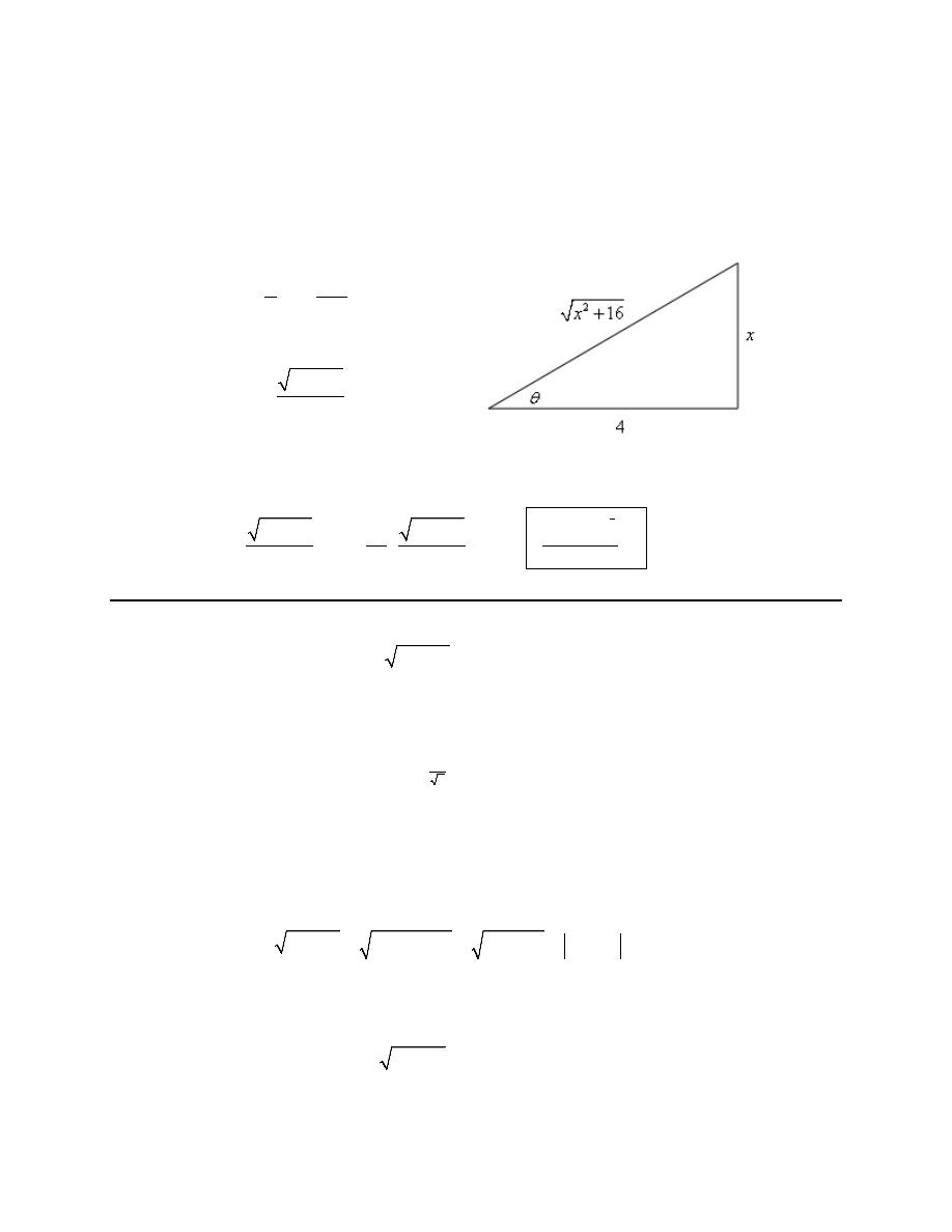
Calculus II
© 2007 Paul Dawkins
33
http://tutorial.math.lamar.edu/terms.aspx
Every trig substitution problem reduces down to an integral involving trig functions and the majority of
them will need some manipulation of the integrand in order to evaluate.
Step 5
As the final step we just need to go back to x’s. To do this we’ll need a quick right triangle. Here is that
work.
From the substitution we have,
( )
opp
tan
4
adj
x
θ
=
=
From the right triangle we get,
( )
2
16
csc
x
x
θ
+
=
The integral is then,
(
)
3
2
3
2
2
2
4
3
16
16
1
16
48
48
x
x
x
dx
c
c
x
x
x
+
+
+
= −
+ = −
+
⌠
⌡
10. Use a trig substitution to evaluate
2
1 7w dw
−
∫
.
Step 1
In this case it looks like we’ll need the following trig substitution.
( )
1
7
sin
w
θ
=
Now we need to use the substitution to eliminate the root and get set up for actually substituting this into
the integral.
Step 2
Let’s first use the substitution to eliminate the root.
( )
( )
( )
2
2
2
1 7
1 sin
cos
cos
w
θ
θ
θ
−
=
−
=
=
Next, because we are doing an indefinite integral we will assume that the cosine is positive and so we can
drop the absolute value bars to get,
( )
2
1 7
cos
w
θ
−
=
Calculus II
© 2007 Paul Dawkins
34
http://tutorial.math.lamar.edu/terms.aspx
For a final substitution preparation step let’s also compute the differential so we don’t forget to use that in
the substitution!
( )
1
7
cos
dw
d
θ θ
=
Step 3
Now let’s do the actual substitution.
( )
( )
(
)
( )
2
2
1
1
7
7
1 7
cos
cos
cos
w dw
d
d
θ
θ
θ
θ θ
−
=
=
∫
∫
∫
Do not forget to substitute in the differential we computed in the previous step. This is probably the most
common mistake with trig substitutions. Forgetting the differential can substantially change the problem,
often making the integral very difficult to evaluate.
Step 4
We now need to evaluate the integral. Here is that work.
( )
( )
2
1
1
1
1
2
2
7
2 7
1 7
1 cos 2
sin 2
w dw
d
c
θ
θ
θ
θ
−
=
+
=
+
+
∫
∫
Don’t forget all the “standard” manipulations of the integrand that we often need to do in order to
evaluate integrals involving trig functions. If you don’t recall them you’ll need to go back to the previous
section and work some practice problems to get good at them.
Every trig substitution problem reduces down to an integral involving trig functions and the majority of
them will need some manipulation of the integrand in order to evaluate.
Step 5
As the final step we just need to go back to w’s.
To eliminate the the first term (i.e. the
θ
) we can use any of the inverse trig functions. The easiest is to
probably just use the original substitution and get a formula involving inverse sine but any of the six trig
functions could be used if we wanted to. Using the substitution gives us,
( )
( )
1
sin
7
sin
7
w
w
θ
θ
−
=
⇒
=
Eliminating the
( )
sin 2
θ
requires a little more work. We can’t just use a right triangle as we normally
would because that would only give trig functions with an argument of
θ
and we have an argument of
2
θ
. However, we could use the double angle formula for sine to reduce this to trig functions with
arguments of
θ
. Doing this gives,
( ) ( )
2
1
2 7
1 7
sin
cos
w dw
c
θ
θ
θ
−
=
+
+
∫
We can now do the right triangle work.
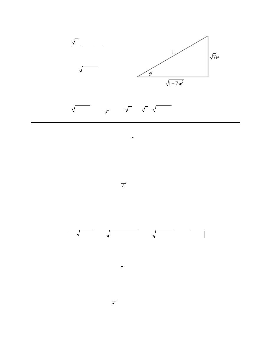
Calculus II
© 2007 Paul Dawkins
35
http://tutorial.math.lamar.edu/terms.aspx
From the substitution we have,
( )
7
opp
sin
1
hyp
w
θ
=
=
From the right triangle we get,
( )
2
cos
1 7w
θ
=
−
The integral is then,
( )
2
1
2
1
2 7
1 7
sin
7
7
1 7
w dw
w
w
w
c
−
−
=
+
−
+
∫
11. Use a trig substitution to evaluate
(
)
5
2
3
2
3
4
t
t
dt
−
∫
.
Step 1
First, do not get excited about the exponent in the integrand. These types of problems work exactly the
same as those with just a root (as opposed to this case in which we have a root to a power – you do agree
that is what we have right?). So, in this case it looks like we’ll need the following trig substitution.
( )
2
3
sec
t
θ
=
Now we need to use the substitution to eliminate the root and get set up for actually substituting this into
the integral.
Step 2
Let’s first use the substitution to eliminate the root.
(
)
( )
( )
( )
5
2
5
5
5
5
2
2
2
2
3
4
3
4
4 sec
4
2 tan
32 tan
t
t
θ
θ
θ
−
=
−
=
−
=
=
Next, because we are doing an indefinite integral we will assume that the tangent is positive and so we
can drop the absolute value bars to get,
(
)
( )
5
2
2
5
3
4
32 tan
t
θ
−
=
For a final substitution preparation step let’s also compute the differential so we don’t forget to use that in
the substitution!
( ) ( )
2
3
sec
tan
dt
d
θ
θ θ
=
Step 3
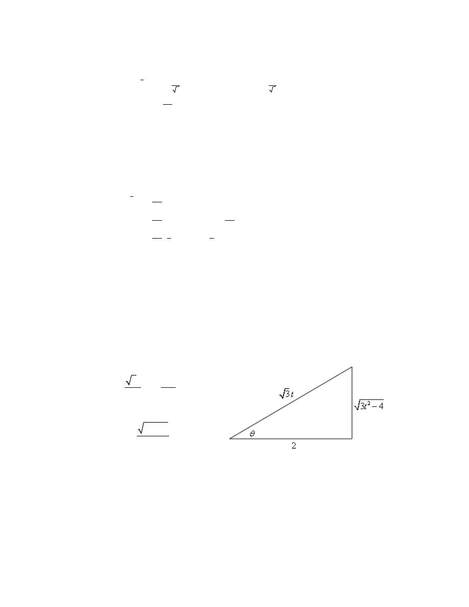
Calculus II
© 2007 Paul Dawkins
36
http://tutorial.math.lamar.edu/terms.aspx
Now let’s do the actual substitution.
(
)
( )
( )
( )
(
)
( ) ( )
(
)
( )
( )
5
2
3
3
2
3
5
2
2
3
3
4
6
512
9
3
4
sec
32 tan
sec
tan
sec
tan
t
t
dt
d
d
θ
θ
θ
θ
θ
θ
θ θ
−
=
=
∫
∫
∫
Do not forget to substitute in the differential we computed in the previous step. This is probably the most
common mistake with trig substitutions. Forgetting the differential can substantially change the problem,
often making the integral very difficult to evaluate.
Step 4
We now need to evaluate the integral. Here is that work.
(
)
( )
(
)
( )
( )
( )
(
)
( )
( )
5
2
3
2
2
6
2
512
9
2
6
8
6
512
512
9
9
9
7
512
1
1
9
9
7
3
4
tan
1 tan
sec
tan
1
tan
tan
t
t
dt
d
u
u
u du
u
u du
c
θ
θ
θ θ
θ
θ
θ
−
=
+
=
=
+
=
+
=
+
+
∫
∫
∫
∫
Don’t forget all the “standard” manipulations of the integrand that we often need to do in order to
evaluate integrals involving trig functions. If you don’t recall them you’ll need to go back to the previous
section and work some practice problems to get good at them.
Every trig substitution problem reduces down to an integral involving trig functions and the majority of
them will need some manipulation of the integrand in order to evaluate.
Step 5
As the final step we just need to go back to t’s. To do this we’ll need a quick right triangle. Here is that
work.
From the substitution we have,
( )
3
hyp
sec
2
adj
t
θ
=
=
From the right triangle we get,
( )
2
3
4
tan
2
t
θ
−
=
The integral is then,
Calculus II
© 2007 Paul Dawkins
37
http://tutorial.math.lamar.edu/terms.aspx
(
)
(
)
(
)
5
2
9
7
2
2
9
7
2
2
3
2
2
2
512 1
3
4
1
3
4
3
4
9
9
2
7
2
3
4
4 3
4
81
63
t
t
t
t
dt
c
t
t
c
−
−
−
=
+
+
−
−
=
+
+
∫
12. Use a trig substitution to evaluate
5
4
2
7
2
25
dy
y
y
−
−
−
⌠
⌡
.
Step 1
In this case it looks like we’ll need the following trig substitution.
( )
5sec
y
θ
=
Now we need to use the substitution to eliminate the root and get set up for actually substituting this into
the integral.
Step 2
Let’s first use the substitution to eliminate the root.
( )
( )
( )
2
2
2
25
25sec
25
5 tan
5 tan
y
θ
θ
θ
−
=
−
=
=
Step 3
Okay, in this case we have limits on y and so we can get limits on
θ
that will allow us to determine if
tangent is positive or negative to allow us to eliminate the absolute value bars.
So, let’s get some limits on
θ
.
( )
( )
( )
( )
( )
1
7
7
5
5
7 :
7
5sec
sec
sec
2.3664
5 :
5
5sec
sec
1
y
y
θ
θ
θ
θ
θ
θ π
−
= −
− =
→
= −
→
=
− =
= −
− =
→
= −
→
=
So,
θ
’s for this problem are in the range
2.3664
θ π
≤ ≤
and these are in the second quadrant. In the
second quadrant we know that tangent is negative and so we can drop the absolute value bars provided we
add in a minus sign. This gives,
( )
2
25
5 tan
y
θ
−
= −
For a final substitution preparation step let’s also compute the differential so we don’t forget to use that in
the substitution!

Calculus II
© 2007 Paul Dawkins
38
http://tutorial.math.lamar.edu/terms.aspx
( ) ( )
5sec
tan
dy
d
θ
θ θ
=
Step 4
Now let’s do the actual substitution.
( )
( )
(
)
( ) ( )
(
)
( )
5
4
4
4
2
2.3664
7
3
2.3664
2
2
5sec
tan
5 sec
5 tan
25
2
1
625
sec
dy
d
y
y
d
π
π
θ
θ
θ
θ
θ
θ
θ
−
−
=
−
−
= −
⌠
⌠
⌡
⌡
⌠
⌡
Do not forget to substitute in the differential we computed in the previous step. This is probably the most
common mistake with trig substitutions. Forgetting the differential can substantially change the problem,
often making the integral very difficult to evaluate.
Also notice that upon doing the substation we replaced the y limits with the
θ
limits. This will help with
a later step.
Step 5
We now need to evaluate the integral. In terms of secants this integral would be pretty difficult, however
we a quick change to cosines we get the following integral.
( )
5
3
4
2
2.3664
7
2
2
cos
625
25
dy
d
y
y
π
θ θ
−
−
= −
−
⌠
⌡
∫
This should be relatively simple to do so here is the integration work.
( )
(
)
( )
( )
(
)
( )
5
2
4
2
2.3664
7
sin
2
2
625
sin 2.3664
0
3
2
1
625
3
0.69986
2
2
1 sin
cos
sin
625
25
1
0.001874
dy
d
u
y
y
u du
u
u
π
π
θ
θ θ
θ
−
−
= −
−
=
−
= −
−
= −
−
=
⌠
⌡
∫
∫
Don’t forget all the “standard” manipulations of the integrand that we often need to do in order to
evaluate integrals involving trig functions. If you don’t recall them you’ll need to go back to the previous
section and work some practice problems to get good at them.
Every trig substitution problem reduces down to an integral involving trig functions and the majority of
them will need some manipulation of the integrand in order to evaluate.
Also, note that because we converted the limits at every substitution into limits for the “new” variable we
did not need to do any back substitution work on our answer!

Calculus II
© 2007 Paul Dawkins
39
http://tutorial.math.lamar.edu/terms.aspx
13. Use a trig substitution to evaluate
4
5
2
1
2
2 9
z
z dz
+
∫
.
Step 1
In this case it looks like we’ll need the following trig substitution.
( )
2
3
tan
z
θ
=
Now we need to use the substitution to eliminate the root and get set up for actually substituting this into
the integral.
Step 2
Let’s first use the substitution to eliminate the root.
( )
( )
( )
2
2
2
2 9
2 2 tan
2 sec
2 sec
z
θ
θ
θ
+
=
+
=
=
Step 3
Okay, in this case we have limits on z and so we can get limits on
θ
that will allow us to determine if
tangent is positive or negative to allow us to eliminate the absolute value bars.
So, let’s get some limits on
θ
.
( )
( )
( )
( )
( )
( )
1
2
3
3
3
2
2
1
2
12
12
3
2
2
1: 1
tan
tan
tan
1.1303
4 : 4
tan
tan
tan
1.4535
z
z
θ
θ
θ
θ
θ
θ
−
−
=
=
→
=
→
=
=
=
=
→
=
→
=
=
So,
θ
’s for this problem are in the range
1.1303
1.4535
θ
≤ ≤
and these are in the first quadrant. In the
first quadrant we know that cosine, and hence secant, is positive and so we can just drop the absolute
value bars. This gives,
( )
2
2 9
2 sec
z
θ
+
=
For a final substitution preparation step let’s also compute the differential so we don’t forget to use that in
the substitution!
( )
2
2
3
sec
dz
d
θ θ
=
Step 4
Now let’s do the actual substitution.
( )
( )
( )
(
)
( )
(
)
( )
( )
1.4535
5
4
5
2
5
2
2
2
3
3
1
1.1303
1.4535
5
3
16 2
729
1.1303
2
2 9
2
tan
2 sec
sec
tan
sec
z
z dz
d
d
θ
θ
θ
θ
θ
θ θ
+
=
=
⌠
⌡
∫
∫

Calculus II
© 2007 Paul Dawkins
40
http://tutorial.math.lamar.edu/terms.aspx
Do not forget to substitute in the differential we computed in the previous step. This is probably the most
common mistake with trig substitutions. Forgetting the differential can substantially change the problem,
often making the integral very difficult to evaluate.
Also notice that upon doing the substation we replaced the y limits with the
θ
limits. This will help with
a later step.
Step 5
We now need to evaluate the integral. Here is that work.
( )
( )
( ) ( )
(
)
(
)
( )
4
1.4535
2
5
2
2
2
16 2
729
1
1.1303
sec 1.4535
2
2
2
16 2
729
sec 1.1303
8.5444
6
4
2
16 2
729
2.3452
8.5444
7
5
3
16 2
1
2
1
729
7
5
3
2.3452
2
2 9
sec
1
sec
tan
sec
1
sec
2
14182.86074
z
z dz
d
u
u du
u
u
u
u du
u
u
u
θ
θ
θ
θ θ
θ
+
=
−
=
−
=
=
−
+
=
−
+
=
∫
∫
∫
∫
Don’t forget all the “standard” manipulations of the integrand that we often need to do in order to
evaluate integrals involving trig functions. If you don’t recall them you’ll need to go back to the previous
section and work some practice problems to get good at them.
Every trig substitution problem reduces down to an integral involving trig functions and the majority of
them will need some manipulation of the integrand in order to evaluate.
Also, note that because we converted the limits at every substitution into limits for the “new” variable we
did not need to do any back substitution work on our answer!
14. Use a trig substitution to evaluate
2
1
9
36
37
dx
x
x
−
+
⌠
⌡
.
Step 1
The first thing we’ll need to do here is complete the square on the polynomial to get this into a form we
can use a trig substitution on.
(
) (
)
(
)
(
)
2
2
2
2
37
37
1
9
9
9
2
9
36
37
9
4
9
4
4 4
9
2
9
2
1
x
x
x
x
x
x
x
x
−
+
=
−
+
=
−
+ − +
=
−
+
=
−
+
The integral is now,
(
)
2
2
1
1
9
36
37
9
2
1
dx
dx
x
x
x
=
−
+
−
+
⌠
⌠
⌡
⌡

Calculus II
© 2007 Paul Dawkins
41
http://tutorial.math.lamar.edu/terms.aspx
Now we can proceed with the trig substitution.
Step 2
It looks like we’ll need to the following trig substitution.
( )
1
3
2
tan
x
θ
− =
Next let’s eliminate the root.
(
)
( )
( )
( )
2
2
2
9
2
1
tan
1
sec
sec
x
θ
θ
θ
−
+ =
+ =
=
Next, because we are doing an indefinite integral we will assume that the secant is positive and so we can
drop the absolute value bars to get,
(
)
( )
2
9
2
1
sec
x
θ
−
+ =
For a final substitution preparation step let’s also compute the differential so we don’t forget to use that in
the substitution!
( )
( )
( )
2
2
1
1
3
3
1
sec
sec
dx
d
dx
d
θ θ
θ θ
=
⇒
=
Recall that all we really need to do here is compute the differential for both the right and left sides of the
substitution.
Step 3
Now let’s do the actual substitution.
( )
( )
( )
2
2
1
1
1
1
sec
sec
sec
3
3
9
36
37
dx
d
d
x
x
θ
θ
θ θ
θ
=
=
−
+
⌠
⌠
⌡
⌡
∫
Do not forget to substitute in the differential we computed in the previous step. This is probably the most
common mistake with trig substitutions. Forgetting the differential can substantially change the problem,
often making the integral very difficult to evaluate.
Step 4
We now need to evaluate the integral. Here is that work.
( )
( )
2
1
1
ln sec
tan
3
9
36
37
dx
c
x
x
θ
θ
=
+
+
−
+
⌠
⌡
Note that this was one of the few trig substitution integrals that didn’t really require a lot of manipulation
of trig functions to completely evaluate. All we had to really do here was use the fact that we determined
the integral of
( )
sec
θ
in the previous section and reuse that result here.
Step 5
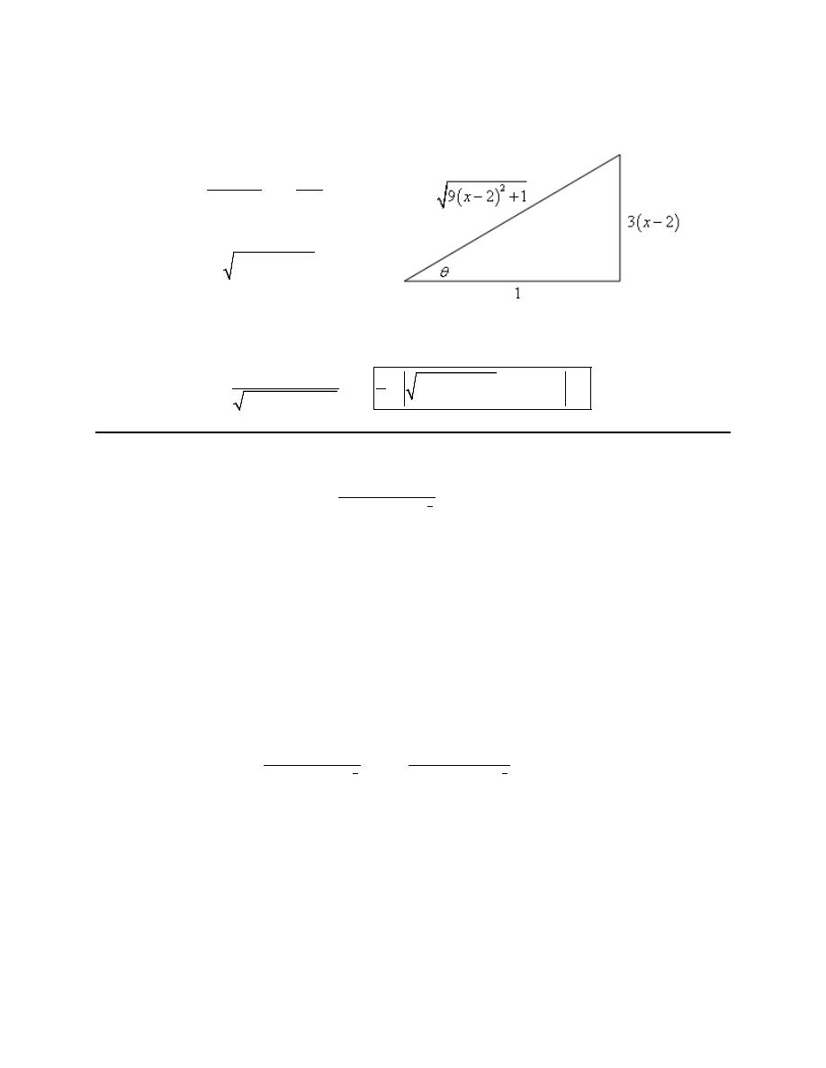
Calculus II
© 2007 Paul Dawkins
42
http://tutorial.math.lamar.edu/terms.aspx
As the final step we just need to go back to x’s. To do this we’ll need a quick right triangle. Here is that
work.
From the substitution we have,
( )
(
)
3
2
opp
tan
1
adj
x
θ
−
=
=
From the right triangle we get,
( )
(
)
2
sec
9
2
1
x
θ
=
−
+
The integral is then,
(
)
(
)
2
2
1
1
ln
9
2
1 3
2
3
9
36
37
dx
x
x
c
x
x
=
−
+ +
−
+
−
+
⌠
⌡
15. Use a trig substitution to evaluate
(
)
(
)
3
2
5
2
3
40 6
z
dz
z
z
+
−
−
⌠
⌡
.
Step 1
The first thing we’ll need to do here is complete the square on the polynomial to get this into a form we
can use a trig substitution on.
(
) (
)
(
)
(
)
2
2
2
2
2
40 6
6
40
6
9 9 40
3
49
49
3
z
z
z
z
z
z
z
z
−
−
= −
+
−
= −
+
+ − −
= −
+
−
=
− +
The integral is now,
(
)
(
)
(
)
(
)
(
)
3
3
2
2
5
5
2
2
3
3
40 6
49
3
z
z
dz
dz
z
z
z
+
+
=
−
−
− +
⌠
⌠
⌡
⌡
Now we can proceed with the trig substitution.
Step 2
It looks like we’ll need to the following trig substitution.
( )
3
7 sin
z
θ
+ =
Next let’s eliminate the root.

Calculus II
© 2007 Paul Dawkins
43
http://tutorial.math.lamar.edu/terms.aspx
(
)
(
)
(
)
( )
( )
( )
3
2
3
3
3
3
2
2
2
49
3
49
3
49 49 sin
7 cos
343 cos
z
z
θ
θ
θ
− +
=
− +
=
−
=
=
Next, because we are doing an indefinite integral we will assume that the cosine is positive and so we can
drop the absolute value bars to get,
(
)
(
)
( )
3
2
2
3
49
3
343cos
z
θ
− +
=
For a final substitution preparation step let’s also compute the differential so we don’t forget to use that in
the substitution!
( )
( )
( )
1
7 cos
7 cos
dz
d
dz
d
θ θ
θ θ
=
⇒
=
Recall that all we really need to do here is compute the differential for both the right and left sides of the
substitution.
Step 3
Now let’s do the actual substitution.
(
)
(
)
( )
( )
( )
(
)
( )
( )
3
2
5
5
5
3
2
2
3
16807 sin
sin
7 cos
343
343cos
cos
40 6
z
dz
d
d
z
z
θ
θ
θ
θ
θ
θ
θ
+
=
=
−
−
⌠
⌠
⌠
⌡
⌡
⌡
Do not forget to substitute in the differential we computed in the previous step. This is probably the most
common mistake with trig substitutions. Forgetting the differential can substantially change the problem,
often making the integral very difficult to evaluate.
Step 4
We now need to evaluate the integral. Here is that work.
(
)
(
)
( )
( )
( )
( )
(
)
( )
( )
( )
3
2
2
5
2
2
2
2
2
2
2
2
1
3
1
3
3
1 cos
3
343
sin
cos
cos
40 6
1
343
343
2
343
2
1
1
343
2 cos
cos
cos
3
z
dz
d
u
z
z
u
du
u
u du
u
u
u
u
c
c
θ
θ θ
θ
θ
θ
θ
θ
−
−
−
+
=
=
−
−
−
= −
= −
− +
= −
−
−
+
+
= −
−
−
+
+
⌠
⌠
⌡
⌡
⌠
⌡
∫
Don’t forget all the “standard” manipulations of the integrand that we often need to do in order to
evaluate integrals involving trig functions. If you don’t recall them you’ll need to go back to the previous
section and work some practice problems to get good at them.
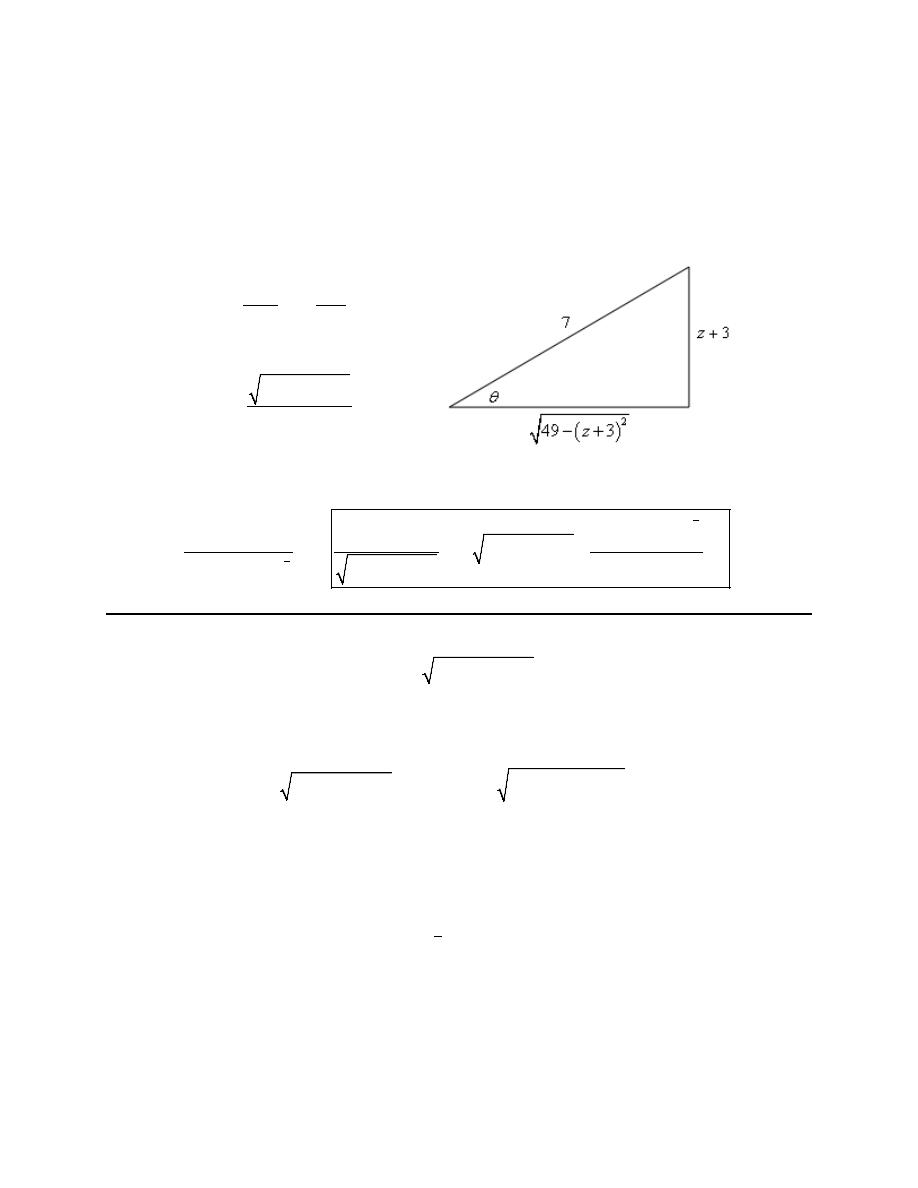
Calculus II
© 2007 Paul Dawkins
44
http://tutorial.math.lamar.edu/terms.aspx
Every trig substitution problem reduces down to an integral involving trig functions and the majority of
them will need some manipulation of the integrand in order to evaluate.
Step 5
As the final step we just need to go back to z’s. To do this we’ll need a quick right triangle. Here is that
work.
From the substitution we have,
( )
3
adj
sin
7
hyp
z
θ
+
=
=
From the right triangle we get,
( )
(
)
2
49
3
cos
7
z
θ
− +
=
The integral is then,
(
)
(
)
(
)
(
)
(
)
(
)
3
2
3
2
2
5
2
2
2
49
3
3
2401
98 49
3
3
49
3
40 6
z
z
dz
z
c
z
z
z
− +
+
=
+
− +
−
+
− +
−
−
⌠
⌡
16. Use a trig substitution to evaluate
( )
( )
2
cos
9
25sin
x
x dx
+
∫
.
Step 1
Let’s first rewrite the integral a little bit.
( )
( )
( )
( )
2
2
cos
9 25sin
cos
9 25 sin
x
x dx
x
x
dx
+
=
+
⌠
⌡
∫
Step 2
With the integral written as it is in the first step we can now see that we do have a sum of a number and
something squared under the root. We know from the problems done previously in this section that looks
like a tangent substitution. So, let’s use the following substitution.
( )
( )
3
5
sin
tan
x
θ
=
Do not get excited about the fact that we are substituting one trig function for another. That will happen
on occasion with these kinds of problems. Note however, that we need to be careful and make sure that
we also change the variable from x (i.e. the variable in the original trig function) into
θ
(i.e. the variable
in the new trig function).

Calculus II
© 2007 Paul Dawkins
45
http://tutorial.math.lamar.edu/terms.aspx
Next let’s eliminate the root.
( )
( )
( )
( )
( )
2
2
2
2
3
5
9 25 sin
9 25
tan
9 9 tan
3 sec
3 sec
x
θ
θ
θ
θ
+
=
+
=
+
=
=
Next, because we are doing an indefinite integral we will assume that the secant is positive and so we can
drop the absolute value bars to get,
( )
( )
2
9 25 sin
3sec
x
θ
+
=
For a final substitution preparation step let’s also compute the differential so we don’t forget to use that in
the substitution!
( )
( )
2
3
5
cos
sec
x dx
d
θ θ
=
Recall that all we really need to do here is compute the differential for both the right and left sides of the
substitution.
Step 3
Now let’s do the actual substitution.
( )
( )
( )
( )
( )
(
)
( )
(
)
( )
2
2
2
3
3
9
5
5
cos
9 25sin
9 25 sin
cos
3sec
sec
sec
x
x dx
x
x dx
d
d
θ
θ
θ
θ θ
+
=
+
=
=
⌠
⌡
∫
∫
∫
Do not forget to substitute in the differential we computed in the previous step. This is probably the most
common mistake with trig substitutions. Forgetting the differential can substantially change the problem,
often making the integral very difficult to evaluate.
Step 4
We now need to evaluate the integral. Here is that work.
( )
( )
( ) ( )
( )
( )
2
9
10
cos
9 25sin
sec
tan
ln sec
tan
x
x dx
c
θ
θ
θ
θ
+
=
+
+
+
∫
Note that this was one of the few trig substitution integrals that didn’t really require a lot of manipulation
of trig functions to completely evaluate. All we had to really do here was use the fact that we determined
the integral of
( )
3
sec
θ
in the previous section and reuse that result here.
Step 5
As the final step we just need to go back to x’s. To do this we’ll need a quick right triangle. Here is that
work.
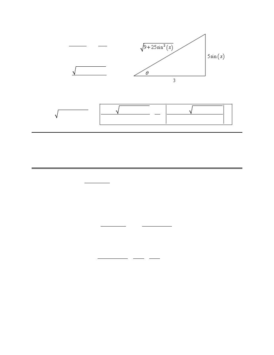
Calculus II
© 2007 Paul Dawkins
46
http://tutorial.math.lamar.edu/terms.aspx
From the substitution we have,
( )
( )
5sin
opp
tan
3
adj
x
θ
=
=
From the right triangle we get,
( )
( )
2
9 25sin
sec
3
x
θ
+
=
The integral is then,
( )
( )
( )
( )
( )
( )
2
2
2
sin
9 25sin
5sin
9 25sin
9
cos
9 25sin
ln
2
10
3
x
x
x
x
x
x dx
c
+
+
+
+
=
+
+
∫
Partial Fractions
1. Evaluate the integral
2
4
5
14
dx
x
x
+
−
⌠
⌡
.
Step 1
To get the problem started off we need the form of the partial fraction decomposition of the integrand.
However, in order to get this we’ll need to factor the denominator.
(
)(
)
2
4
4
5
14
7
2
dx
dx
x
x
x
x
=
+
−
+
−
⌠
⌠
⌡
⌡
The form of the partial fraction decomposition for the integrand is then,
(
)(
)
4
7
2
7
2
A
B
x
x
x
x
=
+
+
−
+
−
Step 2
Setting the numerators equal gives,
(
)
(
)
4
2
7
A x
B x
=
− +
+
Step 3
We can use the “trick” discussed in the notes to easily get the coefficients in this case so let’s do that.
Here is that work.

Calculus II
© 2007 Paul Dawkins
47
http://tutorial.math.lamar.edu/terms.aspx
4
9
4
9
2 :
4
9
7 : 4
9
A
x
B
B
x
A
= −
=
=
⇒
=
= −
= −
The partial fraction form of the integrand is then,
(
)(
)
4
4
9
9
4
7
2
7
2
x
x
x
x
−
=
+
+
−
+
−
Step 4
We can now do the integral.
(
)(
)
4
4
9
9
4
4
4
ln
2
ln
7
7
2
7
2
9
9
dx
dx
x
x
c
x
x
x
x
−
=
+
=
− −
+ +
+
−
+
−
⌠
⌠
⌡
⌡
2. Evaluate the integral
2
8 3
10
13
3
t
dt
t
t
−
+
−
⌠
⌡
.
Step 1
To get the problem started off we need the form of the partial fraction decomposition of the integrand.
However, in order to get this we’ll need to factor the denominator.
(
)(
)
2
8 3
8 3
10
13
3
2
3 5
1
t
t
dt
dt
t
t
t
t
−
−
=
+
−
+
−
⌠
⌠
⌡
⌡
The form of the partial fraction decomposition for the integrand is then,
2
8 3
10
13
3
2
3
5
1
t
A
B
t
t
t
t
−
=
+
+
−
+
−
Step 2
Setting the numerators equal gives,
(
)
(
)
8 3
5
1
2
3
t
A
t
B
t
− =
− +
+
Step 3
We can use the “trick” discussed in the notes to easily get the coefficients in this case so let’s do that.
Here is that work.
25
37
17
1
17
5
5
5
37
3
25
17
17
2
2
2
:
:
A
t
B
B
t
A
= −
=
=
⇒
=
= −
= −
The partial fraction form of the integrand is then,

Calculus II
© 2007 Paul Dawkins
48
http://tutorial.math.lamar.edu/terms.aspx
25
37
17
17
2
8 3
10
13
3
2
3
5
1
t
t
t
t
t
−
−
=
+
+
−
+
−
Step 4
We can now do the integral.
25
37
17
17
2
8 3
37
25
ln 5
1
ln 2
3
10
13
3
2
3
5
1
85
34
t
dt
dt
t
t
c
t
t
t
t
−
−
=
+
=
− −
+ +
+
−
+
−
⌠
⌠
⌡
⌡
Hopefully you are getting good enough with integration that you can do some of these integrals in your
head. Be careful however with both of these integrals. When doing these kinds of integrals in our head it
is easy to forget about the substitutions that are technically required to do them and then miss the
coefficients from the substitutions that need to show up in the answer.
3. Evaluate the integral
(
)(
)(
)
0
2
1
7
2
1
4
w
w
dw
w
w
w
−
+
+
−
−
⌠
⌡
.
Step 1
In this case the denominator is already factored and so we can go straight to the form of the partial
fraction decomposition for the integrand.
(
)(
)(
)
2
7
2
1
4
2
1
4
w
w
A
B
C
w
w
w
w
w
w
+
=
+
+
+
−
−
+
−
−
Step 2
Setting the numerators equal gives,
(
)(
)
(
)(
)
(
)(
)
2
7
1
4
2
4
2
1
w
w
A w
w
B w
w
C w
w
+
=
−
− +
+
− +
+
−
Step 3
We can use the “trick” discussed in the notes to easily get the coefficients in this case so let’s do that.
Here is that work.
5
9
8
9
22
9
1:
8
9
4 :
44 18
2 :
10 18
w
B
A
w
C
B
w
A
C
=
= −
= −
=
=
⇒
= −
= −
− =
=
The partial fraction form of the integrand is then,
(
)(
)(
)
2
5
8
22
9
9
9
7
2
1
4
2
1
4
w
w
w
w
w
w
w
w
−
+
=
−
+
+
−
−
+
−
−

Calculus II
© 2007 Paul Dawkins
49
http://tutorial.math.lamar.edu/terms.aspx
Step 4
We can now do the integral.
(
)(
)(
)
(
)
( )
( )
( )
( )
( )
0
0
2
5
8
22
9
9
9
1
1
0
5
8
22
9
9
9
1
3
47
22
22
22
9
9
9
9
9
7
2
1
4
2
1
4
ln
2
ln
1
ln
4
ln 4
ln 2
ln 5
ln 2
ln 5
w
w
dw
dw
w
w
w
w
w
w
w
w
w
−
−
−
−
+
=
−
+
+
−
−
+
−
−
= −
+ −
− +
−
=
+
−
=
−
⌠
⌠
⌡
⌡
Note that we used a quick logarithm property to combine the first two logarithms into a single logarithm.
You should probably review your logarithm properties if you don’t recognize the one that we used. These
kinds of property applications can really simplify your work on occasion if you know them!
4. Evaluate the integral
3
2
8
3
7
4
dx
x
x
x
+
+
⌠
⌡
.
Step 1
To get the problem started off we need the form of the partial fraction decomposition of the integrand.
However, in order to get this we’ll need to factor the denominator.
(
)(
)
3
2
8
8
3
7
4
3
4
1
dx
dx
x
x
x
x
x
x
=
+
+
+
+
⌠
⌠
⌡
⌡
The form of the partial fraction decomposition for the integrand is then,
(
)(
)
8
3
4
1
3
4
1
A
B
C
x
x
x
x
x
x
= +
+
+
+
+
+
Step 2
Setting the numerators equal gives,
(
)(
)
(
)
(
)
8
3
4
1
1
3
4
A
x
x
Bx x
C x
x
=
+
+ +
+ +
+
Step 3
We can use the “trick” discussed in the notes to easily get the coefficients in this case so let’s do that.
Here is that work.
4
4
3
9
: 8
2
1:
8
18
0 :
8
4
8
x
B
A
x
C
B
x
A
C
= −
=
=
= −
= −
⇒
=
=
=
= −

Calculus II
© 2007 Paul Dawkins
50
http://tutorial.math.lamar.edu/terms.aspx
The partial fraction form of the integrand is then,
(
)(
)
8
2
18
8
3
4
1
3
4
1
x
x
x
x
x
x
= +
−
+
+
+
+
Step 4
We can now do the integral.
(
)(
)
8
2
18
8
2 ln
6 ln 3
4
8 ln
1
3
4
1
3
4
1
dx
dx
x
x
x
c
x
x
x
x
x
x
=
+
−
=
+
+ −
+ +
+
+
+
+
⌠
⌠
⌡
⌡
Hopefully you are getting good enough with integration that you can do some of these integrals in your
head. Be careful however with the second integral. When doing these kinds of integrals in our head it is
easy to forget about the substitutions that are technically required to do them and then miss the
coefficients from the substitutions that need to show up in the answer.
5. Evaluate the integral
(
)(
)
4
2
2
2
3
1
1
5
z
dz
z
z
+
+
−
⌠
⌡
.
Step 1
In this case the denominator is already factored and so we can go straight to the form of the partial
fraction decomposition for the integrand.
(
)(
)
(
)
2
2
2
3
1
1
5
1
5
5
z
A
B
C
z
z
z
z
z
+
=
+
+
+
−
+
−
−
Step 2
Setting the numerators equal gives,
(
)
(
)(
)
(
)
2
2
3
1
5
1
5
1
z
A z
B z
z
C z
+ =
−
+
+
− +
+
Step 3
We can use the “trick” discussed in the notes to easily get two of the coefficients and then we can just
pick another value of z to get the third so let’s do that. Here is that work.
1
9
26
9
139
38
9
3
1:
4
36
5 :
76
6
0 :
1
25
5
5
z
A
A
z
C
B
z
A
B C
B
C
= −
=
=
=
=
⇒
=
=
=
−
+ =
−
=
The partial fraction form of the integrand is then,

Calculus II
© 2007 Paul Dawkins
51
http://tutorial.math.lamar.edu/terms.aspx
(
)(
)
(
)
2
26
38
1
9
9
3
2
2
3
1
1
5
1
5
5
z
z
z
z
z
z
+
=
+
+
+
−
+
−
−
Step 4
We can now do the integral.
(
)(
)
(
)
( )
( )
4
4
2
26
38
1
9
9
3
2
2
2
2
4
38
3
26
27
76
1
1
9
9
9
9
9
2
3
1
1
5
1
5
5
ln
1
ln
5
ln 5
ln 3
5
z
dz
dz
z
z
z
z
z
z
z
z
+
=
+
+
+
−
+
−
−
=
+ +
− −
=
−
+
−
⌠
⌠
⌡
⌡
6. Evaluate the integral
3
2
4
11
9
x
dx
x
x
−
−
⌠
⌡
.
Step 1
To get the problem started off we need the form of the partial fraction decomposition of the integrand.
However, in order to get this we’ll need to factor the denominator.
(
)
3
2
2
4
11
4
11
9
9
x
x
dx
dx
x
x
x
x
−
−
=
−
−
⌠
⌠
⌡
⌡
The form of the partial fraction decomposition for the integrand is then,
(
)
2
2
4
11
9
9
x
A
B
C
x
x
x
x
x
−
= +
+
−
−
Step 2
Setting the numerators equal gives,
(
)
(
)
2
4
11
9
9
x
Ax x
B x
C x
− =
− +
− +
Step 3
We can use the “trick” discussed in the notes to easily get two of the coefficients and then we can just
pick another value of x to get the third so let’s do that. Here is that work.
25
81
11
9
767
25
81
81
0 :
11
9
9 :
25
81
1:
7
8
8
8
x
B
A
x
C
B
x
A
B C
A
C
=
− = −
= −
=
=
⇒
=
=
− = −
−
+ = −
−
=
The partial fraction form of the integrand is then,

Calculus II
© 2007 Paul Dawkins
52
http://tutorial.math.lamar.edu/terms.aspx
(
)
25
25
11
81
9
81
2
2
4
11
9
9
x
x
x
x
x
x
−
−
=
+
+
−
−
Step 4
We can now do the integral.
(
)
25
25
11
11
81
9
81
9
25
25
81
81
2
2
4
11
ln
ln
9
9
9
x
dx
dx
x
x
c
x
x
x
x
x
x
−
−
=
+
+
= −
− +
− +
−
−
⌠
⌠
⌡
⌡
7. Evaluate the integral
(
)
(
)
2
2
2
3
6
4
z
z
dz
z
z
+
+
−
+
⌠
⌡
.
Step 1
In this case the denominator is already factored and so we can go straight to the form of the partial
fraction decomposition for the integrand.
(
)
(
)
2
2
2
2
3
6
4
6
4
z
z
A
Bz
C
z
z
z
z
+
+
+
=
+
−
+
−
+
Step 2
Setting the numerators equal gives,
(
)
(
)(
) (
)
(
)
2
2
2
2
3
4
6
6
4
6
z
z
A z
Bz C
z
A B z
B C z
A
C
+
+ =
+ +
+
−
=
+
+ −
+
+
−
In this case the “trick” discussed in the notes won’t work all that well for us and so we’ll have to resort to
multiplying everything out and collecting like terms as shown above.
Step 3
Now, setting the coefficients equal gives the following system.
2
51
40
1
11
40
0
7
20
:
1
:
6
2
:
4
6
3
z
A
B
A
z
B C
B
z
A
C
C
+ =
=
−
+ =
⇒
= −
−
=
=
The partial fraction form of the integrand is then,
(
)
(
)
2
51
7
11
40
40
20
2
2
2
3
6
4
6
4
z
z
z
z
z
z
z
−
+
+
+
=
+
−
+
−
+
Step 4
We can now do the integral.

Calculus II
© 2007 Paul Dawkins
53
http://tutorial.math.lamar.edu/terms.aspx
(
)
(
)
( )
2
51
7
11
40
40
20
2
2
51
7
11
40
40
20
2
2
2
1
51
7
11
40
80
40
2
2
3
6
4
6
4
6
4
4
ln
6
ln
4
tan
z
z
z
z
dz
dz
z
z
z
z
z
dz
z
z
z
z
z
c
−
−
+
+
+
=
+
−
+
−
+
−
=
+
+
−
+
+
=
− −
+ +
+
⌠
⌠
⌡
⌡
⌠
⌡
Note that the second integration needed the substitution
2
4
u
z
=
+
while the third needed the formula
provided in the notes.
8. Evaluate the integral
(
)(
)
2
3
2
2
8
6
12
3
4
7
t
t
t
dt
t
t
+ +
−
+
+
⌠
⌡
.
Step 1
In this case the denominator is already factored and so we can go straight to the form of the partial
fraction decomposition for the integrand.
(
)(
)
2
3
2
2
2
2
8
6
12
3
4
7
3
4
7
t
t
t
At
B
Ct
D
t
t
t
t
+ +
−
+
+
=
+
+
+
+
+
Step 2
Setting the numerators equal gives,
(
)
(
)
(
)
(
)
(
)
(
)
(
)
2
3
2
2
3
2
8
6
12
7
3
4
3
3
7
4
7
4
t
t
t
At
B t
Ct
D
t
A
C t
B
D t
A
C t
B
D
+ +
−
=
+
+ +
+
+
=
+
+
+
+
+
+
+
In this case the “trick” discussed in the notes won’t work all that well for us and so we’ll have to resort to
multiplying everything out and collecting like terms as shown above.
Step 3
Now, setting the coefficients equal gives the following system.
3
2
1
0
3
:
3
12
0
:
3
6
5
:
7
4
1
2
: 7
4
8
A
t
A
C
B
t
B
D
C
t
A
C
D
t
B
D
=
+
= −
=
+
=
⇒
= −
+
=
=
+
=
The partial fraction form of the integrand is then,

Calculus II
© 2007 Paul Dawkins
54
http://tutorial.math.lamar.edu/terms.aspx
(
)(
)
2
3
2
2
2
2
8
6
12
3
5
2
3
4
7
3
4
7
t
t
t
t
t
t
t
t
t
+ +
−
− +
=
+
+
+
+
+
Step 4
We can now do the integral.
(
)(
)
( )
2
3
2
2
2
2
2
2
2
2
2
1
5
1
2
2
2
7
7
8
6
12
3
5
2
3
4
7
3
4
7
3
5
2
3
4
7
7
ln 3
4
ln
7
tan
t
t
t
t
t
t
dt
dt
t
t
t
t
t
t
dt
t
t
t
t
t
c
−
+ +
−
− +
=
+
+
+
+
+
=
−
+
+
+
+
=
+ −
+ +
+
⌠
⌠
⌡
⌡
⌠
⌡
Note that the first and second integrations needed the substitutions
2
3
4
u
t
=
+
and
2
7
u
t
= +
respectively while the third needed the formula provided in the notes.
9. Evaluate the integral
(
)(
)
2
6
3
2
4
x
x
dx
x
x
−
−
+
⌠
⌡
.
Hint : Pay attention to the degree of the numerator and denominator!
Step 1
Remember that we can only do partial fractions on a rational expression if the degree of the numerator is
less than the degree of the denominator. In this case both the numerator and denominator are both degree
2. This can be easily seen if we multiply the denominator out.
(
)(
)
2
2
2
6
3
6
3
2
4
2
8
x
x
x
x
x
x
x
x
−
−
=
−
+
+
−
So, the first step is to do long division (we’ll leave it up to you to check our Algebra skills for the long
division) to get,
(
)(
)
(
)(
)
2
6
3
48 15
6
2
4
2
4
x
x
x
x
x
x
x
−
−
= +
−
+
−
+
Step 2
Now we can do the partial fractions on the second term. Here is the form of the partial fraction
decomposition.
(
)(
)
48 15
2
4
2
4
x
A
B
x
x
x
x
−
=
+
−
+
−
+

Calculus II
© 2007 Paul Dawkins
55
http://tutorial.math.lamar.edu/terms.aspx
Setting the numerators equal gives,
(
)
(
)
48 15
4
2
x
A x
B x
−
=
+ +
−
Step 3
The “trick” will work here easily enough so here is that work.
4 : 108
6
3
2 :
18
6
18
x
B
A
x
A
B
= −
= −
=
⇒
=
=
= −
The partial fraction form of the second term is then,
(
)(
)
48 15
3
18
2
4
2
4
x
x
x
x
x
−
=
−
−
+
−
+
Step 4
We can now do the integral.
(
)(
)
2
6
3
3
18
6
6
3ln
2
18 ln
4
2
4
2
4
x
x
dx
dx
x
x
x
c
x
x
x
x
−
=
+
−
=
+
− −
+ +
−
+
−
+
⌠
⌠
⌡
⌡
10. Evaluate the integral
4
3
2
9
w
dw
w
w
+
+
⌠
⌡
.
Hint : Pay attention to the degree of the numerator and denominator!
Step 1
Remember that we can only do partial fractions on a rational expression if the degree of the numerator is
less than the degree of the denominator. In this case the degree of the numerator is 4 and the degree of
the denominator is 3.
So, the first step is to do long division (we’ll leave it up to you to check our Algebra skills for the long
division) to get,
(
)
4
2
3
2
2
2 9
9
9
w
w
w
w
w
w w
+
−
= +
+
+
Step 2
Now we can do the partial fractions on the second term. Here is the form of the partial fraction
decomposition.

Calculus II
© 2007 Paul Dawkins
56
http://tutorial.math.lamar.edu/terms.aspx
(
)
2
2
2
2 9
9
9
w
A
Bw C
w
w
w w
−
+
= +
+
+
Setting the numerators equal gives,
(
)
(
) (
)
2
2
2
2 9
9
9
w
A w
w Bw C
A B w
Cw
A
−
=
+ +
+
=
+
+
+
In this case the “trick” discussed in the notes won’t work all that well for us and so we’ll have to resort to
multiplying everything out and collecting like terms as shown above.
Step 3
Now, setting the coefficients equal gives the following system.
2
2
9
1
83
9
0
:
9
:
0
:
9
2
0
w
A
B
A
w
C
B
w
A
C
+ = −
=
=
⇒
= −
=
=
The partial fraction form of the second term is then,
(
)
2
83
2
9
9
2
2
2 9
9
9
w
w
w
w
w w
−
= −
+
+
Step 4
We can now do the integral.
4
83
2
2
2
9
9
83
1
2
2
9
18
3
2
2
ln
ln
9
9
9
w
w
dw
w
dw
w
w
w
c
w
w
w
w
+
=
+ −
=
+
−
+ +
+
+
⌠
⌠
⌡
⌡
Integrals Involving Roots
1. Evaluate the integral
7
2
4
dx
x
+
−
⌠
⌡
.
Step 1
The substitution we’ll use here is,
4
u
x
=
−
Step 2

Calculus II
© 2007 Paul Dawkins
57
http://tutorial.math.lamar.edu/terms.aspx
Now we need to get set up for the substitution. In other words, we need so solve for x and get dx.
2
4
2
x
u
dx
u du
=
+
⇒
=
Step 3
Doing the substitution gives,
( )
7
7
14
2
2
2
2
4
u
dx
u du
du
u
u
x
=
=
+
+
+
−
⌠
⌠
⌠
⌡
⌡
⌡
Step 4
This new integral can be done with the substitution
2
v
u
= +
. Doing this gives,
(
)
14
2
7
28
14
14
28 ln
2
4
v
dx
dv
dv
v
v
c
v
v
x
−
=
=
−
=
−
+
+
−
⌠
⌠
⌠
⌡
⌡
⌡
Step 5
The last step is to now do all the back substitutions to get the final answer.
(
)
(
)
7
14
2
28 ln
2
14
4
2
28 ln
4
2
2
4
dx
u
u
c
x
x
c
x
=
+ −
+ + =
− + −
− + +
+
−
⌠
⌡
Note that we could have avoided the second substitution if we’d used
4
2
u
x
=
− +
for the original
substitution.
This often doesn’t work, but in this case because the only extra term in the denominator was a constant it
didn’t change the differential work and so would work pretty easily for this problem.
2. Evaluate the integral
1
2 1
2
dw
w
w
+
− +
⌠
⌡
.
Step 1
The substitution we’ll use here is,
1
u
w
=
−
Step 2
Now we need to get set up for the substitution. In other words, we need so solve for w and get dw.
2
1
2
w
u
dw
u du
= −
⇒
= −
Step 3
Doing the substitution gives,

Calculus II
© 2007 Paul Dawkins
58
http://tutorial.math.lamar.edu/terms.aspx
(
)
2
2
1
1
2
2
1
2
2
2
3
2 1
2
u
dw
u du
du
u
u
u
u
w
w
=
−
=
−
+
+
−
−
+
− +
⌠
⌠
⌠
⌡
⌡
⌡
Step 4
This integral requires partial fractions to evaluate. Let’s start with the form of the partial fraction
decomposition.
(
)(
)
2
1
3
1
3
u
A
B
u
u
u
u
=
+
+
−
+
−
Setting the coefficients equal gives,
(
)
(
)
2
3
1
u
A u
B u
=
− +
+
Using the “trick” to get the coefficients gives,
1
2
3
2
3 :
6
4
1:
2
4
A
u
B
B
u
A
=
=
=
⇒
=
= −
− = −
The integral is then,
(
)(
)
3
1
2
2
2
1
3
ln
1
ln
3
1
3
1
3
2
2
u
du
du
u
u
c
u
u
u
u
=
+
=
+ +
− +
+
−
+
−
⌠
⌠
⌡
⌡
Step 5
The last step is to now do all the back substitutions to get the final answer.
1
1
3
ln 1
1
ln 1
3
2
2
2 1
2
dw
w
w
c
w
w
=
− + +
− − +
+
− +
⌠
⌡
3. Evaluate the integral
2
3 2
4
2
t
dt
t
t
−
−
− +
⌠
⌡
.
Step 1
The substitution we’ll use here is,
2
4
u
t
=
−
Step 2
Now we need to get set up for the substitution. In other words, we need so solve for t and get dt.
2
1
2
2
t
u
dt
u du
=
+
⇒
=

Calculus II
© 2007 Paul Dawkins
59
http://tutorial.math.lamar.edu/terms.aspx
Step 3
Doing the substitution gives,
( )
2
3
1
2
2
2
1
2
2 2
2
2 3
2
6
8
3 2
4
2
u
t
u
dt
u du
du
u
u
u
u
t
t
+ −
−
=
=
+ −
+
−
+
−
− +
⌠
⌠
⌠
⌡
⌡
⌡
Step 4
This integral requires partial fractions to evaluate.
However, we first need to do long division on the integrand since the degree of the numerator (3) is
higher than the degree of the denominator (2). This gives,
(
)(
)
3
2
28
48
6
6
8
2
4
u
u
u
u
u
u
u
−
= + +
−
+
−
−
The form of the partial fraction decomposition on the third term is,
(
)(
)
28
48
2
4
2
4
u
A
B
u
u
u
u
−
=
+
−
−
−
−
Setting the coefficients equal gives,
(
)
(
)
28
48
4
2
u
A u
B u
−
=
− +
−
Using the “trick” to get the coefficients gives,
4 : 64
2
4
2 :
8
2
32
u
B
A
u
A
B
=
=
= −
⇒
=
= −
=
The integral is then,
3
2
2
4
32
1
6
6
4 ln
2
32 ln
4
6
8
2
4
2
u
du
u
du
u
u
u
u
c
u
u
u
u
=
+ −
+
=
+
−
− +
− +
−
+
−
−
⌠
⌠
⌡
⌡
Step 5
The last step is to now do all the back substitutions to get the final answer.
3
2
2 6 2
4
4 ln
2
4
2
32 ln
2
4
4
6
8
u
du
t
t
t
t
c
u
u
= − +
− −
− − +
− − +
−
+
⌠
⌡
Calculus II
© 2007 Paul Dawkins
60
http://tutorial.math.lamar.edu/terms.aspx
Integrals Involving Quadratics
1. Evaluate the integral
2
7
3
3
dw
w
w
+
+
⌠
⌡
.
Step 1
The first thing to do is to complete the square (we’ll leave it to you to verify the completing the square
details) on the quadratic in the denominator.
(
)
2
2
3
3
2
4
7
7
3
3
dw
dw
w
w
w
=
+
+
+
+
⌠
⌠
⌡
⌡
Step 2
From this we can see that the following substitution should work for us.
3
2
u
w
du
dw
= +
⇒
=
Doing the substitution gives,
2
2
3
4
7
7
3
3
dw
du
w
w
u
=
+
+
+
⌠
⌠
⌡
⌡
Step 3
This integral can be done with the formula given at the start of this section.
1
1
2
7
14
2
14
2
3
tan
tan
3
3
3
3
3
3
u
w
dw
c
c
w
w
−
−
+
=
+ =
+
+
+
⌠
⌡
Don’t forget to back substitute in for u!
2. Evaluate the integral
2
10
4
8
9
x
dx
x
x
−
+
⌠
⌡
.
Step 1
The first thing to do is to complete the square (we’ll leave it to you to verify the completing the square
details) on the quadratic in the denominator.
(
)
2
2
10
10
4
8
9
4
1
5
x
x
dx
dx
x
x
x
=
−
+
−
+
⌠
⌠
⌡
⌡
Step 2
From this we can see that the following substitution should work for us.
Calculus II
© 2007 Paul Dawkins
61
http://tutorial.math.lamar.edu/terms.aspx
1
&
1
u
x
du
dx
x
u
= −
⇒
=
= +
Doing the substitution gives,
(
)
2
2
10
1
10
4
8
9
4
5
u
x
dx
du
x
x
u
+
=
−
+
+
⌠
⌠
⌡
⌡
Step 3
We can quickly do this integral if we split it up as follows,
2
2
2
2
2
5
4
10
10
10
10
5
1
4
8
9
4
5
4
5
4
5
2
x
u
u
dx
du
du
du
du
x
x
u
u
u
u
=
+
=
+
−
+
+
+
+
+
⌠
⌠
⌠
⌠
⌠
⌡
⌡
⌡
⌡
⌡
After a quick rewrite of the second integral we can see that we can do the first with the substitution
2
4
5
v
u
=
+
and the second is an inverse trig integral we can evaluate using the formula given at the start
of the notes for this section.
(
)
1
2
2
1
2
1
10
5
5
2
2
ln
tan
4
8
9
4
2
5
5
5
2
ln 4
5
5 tan
4
5
5
2
2
ln 4
1
5
5 tan
4
5
x
u
dx
v
c
x
x
u
u
c
x
x
c
−
−
−
=
+
+
−
+
=
+ +
+
−
=
−
+ +
+
⌠
⌡
Don’t forget to back substitute in for u!
3. Evaluate the integral
(
)
5
2
2
2
9
14
46
t
dt
t
t
+
−
+
⌠
⌡
.
Step 1
The first thing to do is to complete the square (we’ll leave it to you to verify the completing the square
details) on the quadratic in the denominator.
(
)
(
)
(
)
5
5
2
2
2
2
2
9
2
9
14
46
7
3
t
t
dt
dt
t
t
t
+
+
=
−
+
−
−
⌠
⌠
⌡
⌡
Step 2
From this we can see that the following substitution should work for us.

Calculus II
© 2007 Paul Dawkins
62
http://tutorial.math.lamar.edu/terms.aspx
7
&
7
u
t
du
dt
t
u
= −
⇒
=
= +
Doing the substitution gives,
(
)
(
)
(
)
(
)
5
5
5
2
2
2
2
2
2
2
7
9
2
9
2
23
14
46
3
3
u
t
u
dt
du
du
t
t
u
u
+
+
+
+
=
=
−
+
−
−
⌠
⌠
⌠
⌡
⌡
⌡
Step 3
Next we’ll need to split the integral up as follows,
(
)
(
)
(
)
5
5
5
2
2
2
2
2
2
2
9
2
23
14
46
3
3
t
u
dt
du
du
t
t
u
u
+
=
+
−
+
−
−
⌠
⌠
⌠
⌡
⌡
⌡
The first integral can be done with the substitution
2
3
v
u
=
−
and the second integral will require the trig
substitution
3 sec
u
θ
=
. Here is the substitution work.
(
)
(
)
(
)
(
)
5
2
5
5
2
2
5
2
5
2
5
2
5
2
2
2
2
4
3
4
2
9
23
3 sec tan
14
46
3sec
3
23 3 sec tan
3 tan
23sec
9 tan
23
cos
9
sin
t
dt
v
dv
d
t
t
v
dv
d
v
dv
d
v
dv
d
θ
θ θ
θ
θ
θ θ
θ
θ θ
θ
θ θ
θ
−
−
−
−
+
=
+
−
+
−
=
+
=
+
=
+
⌠
⌠
⌡
⌡
⌠
⌡
⌠
⌡
⌠
⌡
∫
∫
∫
∫
Now, for the second integral, don’t forget the manipulations we often need to do so we can do these kinds
of integrals. If you need some practice on these kinds of integrals go back to the practice problems for the
second section of this chapter and work some of them.
Here is the rest of the integration process for this problem.
(
)
(
) (
)
5
2
5
2
5
2
3
2
2
4
2
4
2
23
9
3
1
23
2
1
3
9
3
2
9
23
1 sin
cos
sin
9
sin
14
46
sin
sin
t
dt
v
dv
d
w
t
t
v
dv
w
w dw
v
c
θ
θ θ
θ
θ
θ
θ
−
−
−
−
−
−
−
+
−
=
+
=
−
+
=
+
−
= −
+
−
+
+
⌠
⌠
⌡
⌡
∫
∫
∫
Step 4
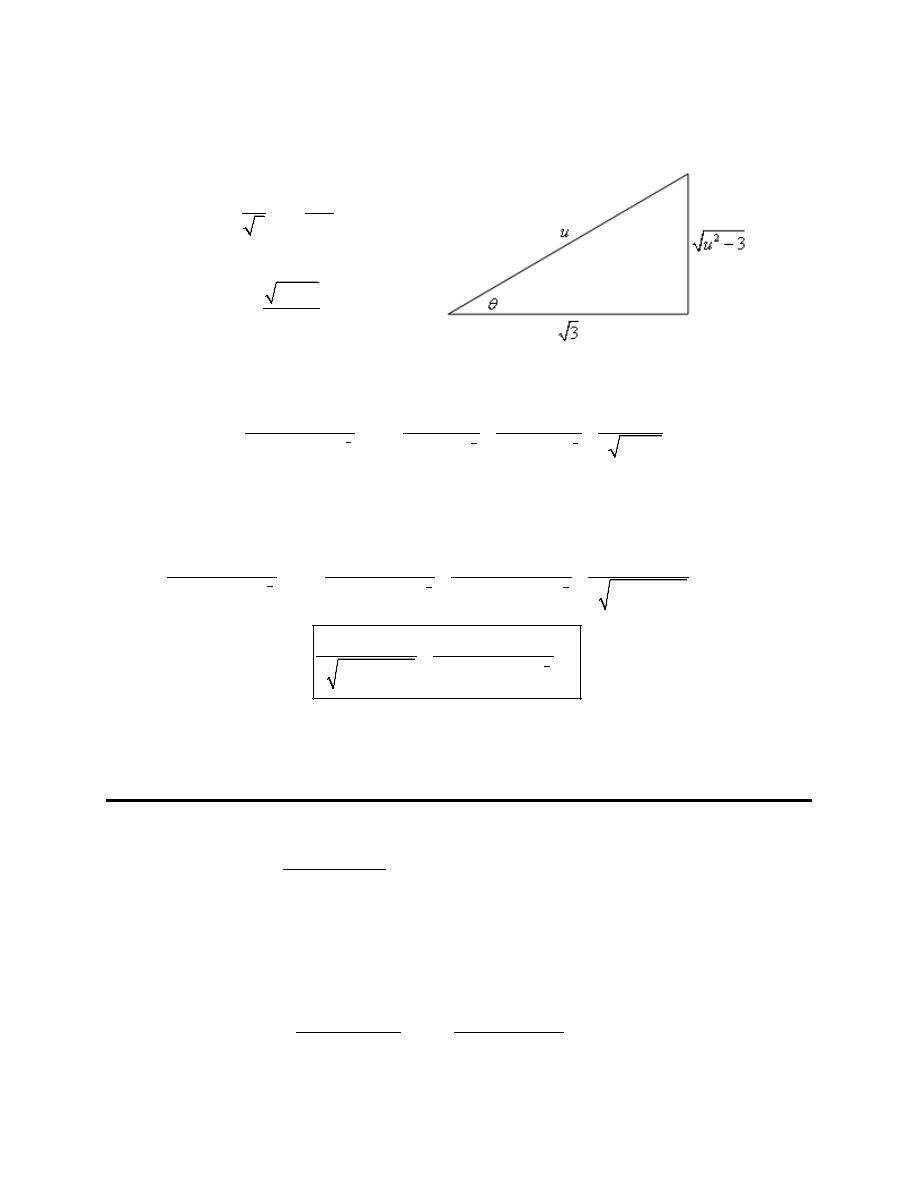
Calculus II
© 2007 Paul Dawkins
63
http://tutorial.math.lamar.edu/terms.aspx
We now need to do quite a bit of back substitution to get the answer back into t’s. Let’s start with the
result of the second integration. Converting the
θ
’s back to u’s will require a quick right triangle.
From the substitution we have,
hyp
sec
adj
3
u
θ
=
=
From the right triangle we get,
2
3
sin
u
u
θ
−
=
Plugging this into the integral above gives,
(
)
(
)
(
)
5
3
3
2
2
2
3
2
2
2
2
2
9
2
23
23
9
3
14
46
3
3
27
3
t
u
u
dt
c
u
t
t
u
u
+
= −
−
+
+
−
−
+
−
−
⌠
⌡
Note that we also back substituted for the v in the first term as well and rewrote the first term a little.
Finally, all we need to do is back substitute for the u.
(
)
(
)
(
)
(
)
(
)
(
)
(
)
(
)
(
)
(
)
(
)
(
)
(
)
5
3
3
2
2
2
3
2
3
2
2
2
2
3
2
2
23
7
23
7
2
9
2
9
7
3
14
46
3
7
3
27
7
3
23
7
18 23
7
9
7
3
27
7
3
t
t
t
dt
c
t
t
t
t
t
t
t
c
t
t
−
−
+
= −
−
+
+
−
−
−
+
−
−
−
−
−
+
−
=
−
+
−
−
−
−
⌠
⌡
We’ll leave this solution with a final note about these kinds of problems. They are often very long, messy
and there are ample opportunities for mistakes so be careful with these and don’t get into too much of a
hurry when working them.
4. Evaluate the integral
(
)
2
2
3
1 4
2
z
dz
z
z
−
−
⌠
⌡
.
Step 1
The first thing to do is to complete the square (we’ll leave it to you to verify the completing the square
details) on the quadratic in the denominator.
(
)
(
)
(
)
2
2
2
2
3
3
1 4
2
3 2
1
z
z
dz
dz
z
z
z
=
−
−
−
+
⌠
⌠
⌡
⌡
Calculus II
© 2007 Paul Dawkins
64
http://tutorial.math.lamar.edu/terms.aspx
Step 2
From this we can see that the following substitution should work for us.
1
&
1
u
z
du
dz
z
u
= +
⇒
=
= −
Doing the substitution gives,
(
)
(
)
(
)
(
)
2
2
2
2
2
2
3
1
3
3
3
1 4
2
3 2
3 2
u
z
u
dz
du
du
z
z
u
u
−
−
=
=
−
−
−
−
⌠
⌠
⌠
⌡
⌡
⌡
Step 3
Next we’ll need to split the integral up as follows,
(
)
(
)
(
)
2
2
2
2
2
2
3
3
3
1 4
2
3 2
3 2
z
u
dz
du
du
z
z
u
u
=
−
−
−
−
−
⌠
⌠
⌠
⌡
⌡
⌡
The first integral can be done with the substitution
2
3 2
v
u
= −
and the second integral will require the
trig substitution
3
2
sin
u
θ
=
. Here is the substitution work.
(
)
(
)
(
)
(
)
(
)
2
3
2
2
2
2
2
2
3
2
2
2
2
3
3
1
4
6
3
3
3
cos
4
1 4
2
3 3sin
3
3
cos
4
3cos
sec
z
dz
v dv
d
z
z
v dv
d
v dv
d
θ θ
θ
θ θ
θ
θ θ
−
−
−
= −
−
−
−
−
= −
−
= −
−
⌠
⌠
⌡
⌡
⌠
⌡
∫
∫
∫
∫
The second integral for this problem comes down to an integral that was done in the notes for the second
section of this chapter and so we’ll just use the formula derived in that section to do this integral.
Here is the rest of the integration process for this problem.
(
)
1
2
2
3
3
1
sec tan
ln sec
tan
4
2 6
1 4
2
z
dz
v
c
z
z
θ
θ
θ
θ
−
=
−
+
+
+
−
−
⌠
⌡
Step 4
We now need to do quite a bit of back substitution to get the answer back into z’s. Let’s start with the
result of the second integration. Converting the
θ
’s back to u’s will require a quick right triangle.
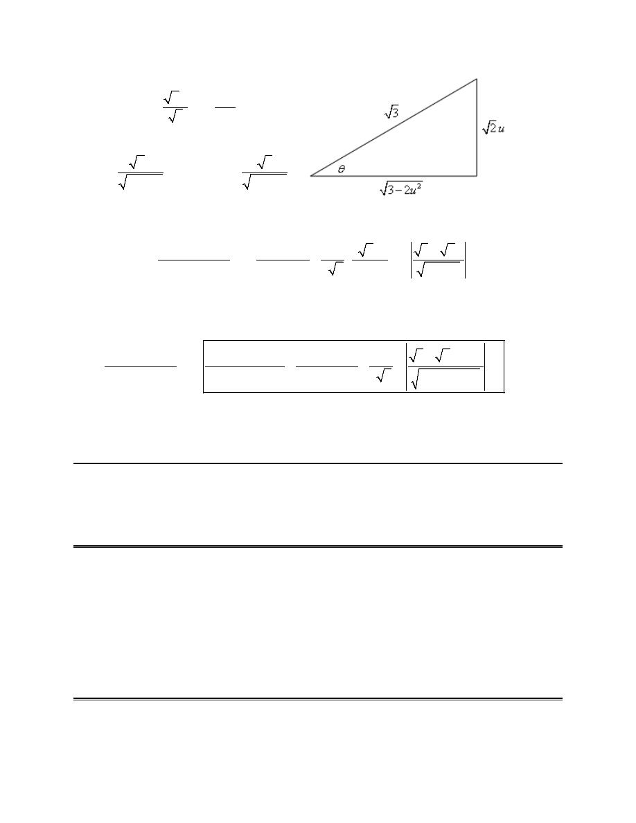
Calculus II
© 2007 Paul Dawkins
65
http://tutorial.math.lamar.edu/terms.aspx
From the substitution we have,
2
opp
sin
hyp
3
u
θ
=
=
From the right triangle we get,
2
2
2
3
tan
&
sec
3 2
3 2
u
u
u
θ
θ
=
=
−
−
Plugging this into the integral above gives,
(
)
(
)
2
2
2
2
2
3
3
1
6
3
2
ln
3 2
4 3 2
2 6
3 2
1 4
2
z
u
u
dz
c
u
u
u
z
z
+
=
−
+
+
−
−
−
−
−
⌠
⌡
Note that we also back substituted for the v in the first term as well and rewrote the first term a little.
Finally, all we need to do is back substitute for the u.
(
)
(
)
(
)
(
)
(
)
(
)
2
2
2
2
2
3
2
1
3
3
1
1
ln
2 6
6 4
1
4 3 2
1
1 4
2
3 2
1
z
z
z
dz
c
z
z
z
z
z
+
+
+
=
−
−
+
−
+
−
+
−
−
−
+
⌠
⌡
We’ll leave this solution with a final note about these kinds of problems. They are often very long, messy
and there are ample opportunities for mistakes so be careful with these and don’t get into too much of a
hurry when working them.
Integration Strategy
Problems have not yet been written for this section.
I was finding it very difficult to come up with a good mix of “new” problems and decided my time was
better spent writing problems for later sections rather than trying to come up with a sufficient number of
problems for what is essentially a review section. I intend to come back at a later date when I have more
time to devote to this section and add problems then.
Improper Integrals
1. Determine if the following integral converges or diverges. If the integral converges determine its
value.

Calculus II
© 2007 Paul Dawkins
66
http://tutorial.math.lamar.edu/terms.aspx
(
)
0
1 2
x
x
dx
∞
−
+
∫
e
Hint : Don’t forget that we can’t do the integral as long as there is an infinity in one of the limits!
Step 1
First, we need to recall that we can’t do the integral as long as there is an infinity in one of the limits.
Therefore, we’ll need to eliminate the infinity first as follows,
(
)
(
)
0
0
1 2
lim
1 2
t
t
x
x
x
dx
x
dx
∞
−
−
→∞
+
=
+
∫
∫
e
e
Note that this step really is needed for these integrals! For some integrals we can use basic logic and
“evaluate” at infinity to get the answer. However, many of these kinds of improper integrals can’t be
done that way! This is the only way to make sure we can deal with the infinite limit in those cases.
So even if this ends up being one of the integrals in which we can “evaluate” at infinity we need to be in
the habit of doing this for those that can’t be done that way.
Step 2
Next, let’s do the integral. We’ll not be putting a lot of explanation/detail into the integration process. By
this point it is assumed that your integration skills are getting pretty good. If you find your integration
skills are a little rusty you should go back and do some practice problems from the appropriate earlier
sections.
In this case we need to do integration by parts to evaluate this integral. Here is the integration work.
1 2
2
x
x
u
x
du
dx
dv
dx
v
−
−
= +
→
=
=
→
= −
e
e
(
)
(
)
(
)
(
)
1 2
1 2
2
1 2
2
3 2
x
x
x
x
x
x
x
dx
x
dx
x
c
x
c
−
−
−
−
−
−
+
= − +
+
= − +
−
+ = − +
+
∫
∫
e
e
e
e
e
e
Note that we didn’t do the definite integral here. The limits don’t really affect how we do the integral and
so we held off dealing with them until the next step.
Step 3
Okay, now let’s take care of the limits on the integral.
(
)
(
)
(
)
(
)
(
)
0
0
1 2
lim
3 2
lim 3
3 2
t
t
t
x
x
t
x
dx
x
t
∞
−
−
−
→∞
→∞
+
=
− +
=
− +
∫
e
e
e
Step 4
We now need to evaluate the limit in our answer from the previous step and note that, in this case, we
really can’t just “evaluate” at infinity! We need to do the limiting process here to make sure we get the
correct answer.
We will need to do a quick L’Hospitals Rule on the second term to properly evaluate it. Here is the limit
work.

Calculus II
© 2007 Paul Dawkins
67
http://tutorial.math.lamar.edu/terms.aspx
(
)
0
3 2
2
1 2
lim 3 lim
3 lim
3 0
3
t
t
t
x
t
t
t
x
dx
∞
−
→∞
→∞
→∞
+
+
=
−
= −
= − =
∫
e
e
e
Step 5
The final step is to write down the answer!
In this case, the limit we computed in the previous step existed and was finite (i.e. not an infinity).
Therefore, the integral converges and its value is 3.
2. Determine if the following integral converges or diverges. If the integral converges determine its
value.
(
)
0
1 2
x
x
dx
−
−∞
+
∫
e
Hint : Don’t forget that we can’t do the integral as long as there is an infinity in one of the limits!
Step 1
First, we need to recall that we can’t do the integral as long as there is an infinity in one of the limits.
Therefore, we’ll need to eliminate the infinity first as follows,
(
)
(
)
0
0
1 2
lim
1 2
t
t
x
x
x
dx
x
dx
−
−
−∞
→−∞
+
=
+
∫
∫
e
e
Note that this step really is needed for these integrals! For some integrals we can use basic logic and
“evaluate” at infinity to get the answer. However, many of these kinds of improper integrals can’t be
done that way! This is the only way to make sure we can deal with the infinite limit in those cases.
So even if this ends up being one of the integrals in which we can “evaluate” at infinity we need to be in
the habit of doing this for those that can’t be done that way.
Step 2
Next, let’s do the integral. We’ll not be putting a lot of explanation/detail into the integration process. By
this point it is assumed that your integration skills are getting pretty good. If you find your integration
skills are a little rusty you should go back and do some practice problems from the appropriate earlier
sections.
In this case we need to do integration by parts to evaluate this integral. Here is the integration work.
1 2
2
x
x
u
x
du
dx
dv
dx
v
−
−
= +
→
=
=
→
= −
e
e
(
)
(
)
(
)
(
)
1 2
1 2
2
1 2
2
3 2
x
x
x
x
x
x
x
dx
x
dx
x
c
x
c
−
−
−
−
−
−
+
= − +
+
= − +
−
+ = − +
+
∫
∫
e
e
e
e
e
e
Note that we didn’t do the definite integral here. The limits don’t really affect how we do the integral and
so we held off dealing with them until the next step.

Calculus II
© 2007 Paul Dawkins
68
http://tutorial.math.lamar.edu/terms.aspx
Step 3
Okay, now let’s take care of the limits on the integral.
(
)
(
)
(
)
(
)
(
)
0
0
1 2
lim
3 2
lim
3 2
3
t
t
t
x
x
t
x
dx
x
t
−
−
−
−∞
→ −∞
→−∞
+
=
− +
=
+
−
∫
e
e
e
Step 4
We now need to evaluate the limit in our answer from the previous step. In this case we can see that the
first term will go to negative infinity since it is just a product of one factor that goes to negative infinity
and another factor that goes to infinity. Therefore the full limit will also be negative infinity since the
constant second term won’t affect the final value of the limit.
(
)
(
)
( )( )
0
1 2
lim 3 2
lim 3
3
3
t
t
x
t
x
dx
t
−
−∞
→−∞
→∞
−
+
=
+
−
= −∞ ∞ − = −∞ − = −∞
∫
e
e
Step 5
The final step is to write down the answer!
In this case, the limit we computed in the previous step existed and but was negative infinity. Therefore,
the integral diverges.
3. Determine if the following integral converges or diverges. If the integral converges determine its
value.
1
5
1
10
2
dz
z
−
+
⌠
⌡
Hint : Don’t forget that we can’t do the integral as long as there is a division by zero in the integrand at
some point in the interval of integration!
Step 1
First, notice that there is a division by zero issue (and hence a discontinuity) in the integrand at
5
z
= −
and this is the lower limit of integration. We know that as long as that discontinuity is there we can’t do
the integral. Therefore, we’ll need to eliminate the discontinuity first as follows,
1
1
5
5
1
1
lim
10 2
10 2
t
t
dz
dz
z
z
+
→−
−
=
+
+
⌠
⌠
⌡
⌡
Don’t forget that the limits on these kinds of integrals must be one-sided limits. Because the interval of
integration is
[
]
5,1
−
we are only interested in the values of z that are greater than -5 and so we must use a
right hand limit to reflect that fact.
Step 2
Next, let’s do the integral. We’ll not be putting a lot of explanation/detail into the integration process. By
this point it is assumed that your integration skills are getting pretty good. If you find your integration
skills are a little rusty you should go back and do some practice problems from the appropriate earlier
sections.

Calculus II
© 2007 Paul Dawkins
69
http://tutorial.math.lamar.edu/terms.aspx
In this case we can do a simple Calc I substitution. Here is the integration work.
1
1
ln 10
2
10
2
2
dz
z
c
z
=
+
+
+
⌠
⌡
Note that we didn’t do the definite integral here. The limits don’t really affect how we do the integral and
so we held off dealing with them until the next step.
Step 3
Okay, now let’s take care of the limits on the integral.
1
1
5
5
5
1
1
1
1
lim
ln 10 2
lim
ln 12
ln 10 2
10 2
2
2
2
t
t
t
dz
z
t
z
+
+
→−
→−
−
=
+
=
−
+
+
⌠
⌡
Step 4
We now need to evaluate the limit in our answer from the previous step. Here is the limit work.
1
5
5
1
1
1
1
lim
ln 12
ln 10
2
ln 12
10
2
2
2
2
t
dz
t
z
+
→−
−
=
−
+
=
+ ∞ = ∞
+
⌠
⌡
Step 5
The final step is to write down the answer!
In this case, the limit we computed in the previous step existed and but was infinity. Therefore, the
integral diverges.
4. Determine if the following integral converges or diverges. If the integral converges determine its
value.
2
3
2
1
4
4
w
dw
w
−
⌠
⌡
Hint : Don’t forget that we can’t do the integral as long as there is a division by zero in the integrand at
some point in the interval of integration!
Step 1
First, notice that there is a division by zero issue (and hence a discontinuity) in the integrand at
2
w
=
and this is the upper limit of integration. We know that as long as that discontinuity is there we can’t do
the integral. Therefore, we’ll need to eliminate the discontinuity first as follows,
2
3
3
2
2
2
1
1
4
4
lim
4
4
t
t
w
w
dw
dw
w
w
−
→
=
−
−
⌠
⌠
⌡
⌡
Calculus II
© 2007 Paul Dawkins
70
http://tutorial.math.lamar.edu/terms.aspx
Don’t forget that the limits on these kinds of integrals must be one-sided limits. Because the interval of
integration is
[ ]
1, 2
we are only interested in the values of t that are less than 2 and so we must use a left
hand limit to reflect that fact.
Step 2
Next, let’s do the integral. We’ll not be putting a lot of explanation/detail into the integration process. By
this point it is assumed that your integration skills are getting pretty good. If you find your integration
skills are a little rusty you should go back and do some practice problems from the appropriate earlier
sections.
In this case we can do a simple Calc I substitution. Here is the integration work.
(
)
2
3
2
3
2
4
3
4
4
w
dw
w
c
w
=
−
+
−
⌠
⌡
Note that we didn’t do the definite integral here. The limits don’t really affect how we do the integral and
so we held off dealing with them until the next step.
Step 3
Okay, now let’s take care of the limits on the integral.
(
)
(
)
(
)
( )
(
)
2
2
2
3
3
3
2
2
2
3
2
2
2
1
1
4
lim 3
4
lim 3
4
3
3
4
t
t
t
w
dw
w
t
w
−
−
→
→
=
−
=
−
− −
−
⌠
⌡
Step 4
We now need to evaluate the limit in our answer from the previous step. Here is the limit work.
(
)
( )
(
)
( ) ( )
2
5
2
2
3
3
3
3
2
2
3
2
2
1
4
lim 3
4
3
3
3
3
3
4
t
w
dw
t
w
−
→
=
−
− −
= − −
= −
−
⌠
⌡
Step 5
The final step is to write down the answer!
In this case, the limit we computed in the previous step existed and was finite (i.e. not an infinity).
Therefore, the integral converges and its value is
( )
5
3
3
−
.
5. Determine if the following integral converges or diverges. If the integral converges determine its
value.
1
6
y dy
−∞
−
∫
Hint : Don’t forget that we can’t do the integral as long as there is an infinity in one of the limits!
Step 1

Calculus II
© 2007 Paul Dawkins
71
http://tutorial.math.lamar.edu/terms.aspx
First, we need to recall that we can’t do the integral as long as there is an infinity in one of the limits.
Therefore, we’ll need to eliminate the infinity first as follows,
1
1
6
lim
6
t
t
y dy
y dy
−∞
→−∞
−
=
−
∫
∫
Note that this step really is needed for these integrals! For some integrals we can use basic logic and
“evaluate” at infinity to get the answer. However, many of these kinds of improper integrals can’t be
done that way! This is the only way to make sure we can deal with the infinite limit in those cases.
So even if this ends up being one of the integrals in which we can “evaluate” at infinity we need to be in
the habit of doing this for those that can’t be done that way.
Step 2
Next, let’s do the integral. We’ll not be putting a lot of explanation/detail into the integration process. By
this point it is assumed that your integration skills are getting pretty good. If you find your integration
skills are a little rusty you should go back and do some practice problems from the appropriate earlier
sections.
In this case we can do a simple Calc I substitution. Here is the integration work.
(
)
3
2
2
3
6
6
y dy
y
c
−
= −
−
+
∫
Note that we didn’t do the definite integral here. The limits don’t really affect how we do the integral and
so we held off dealing with them until the next step.
Step 3
Okay, now let’s take care of the limits on the integral.
(
)
(
)
( )
(
)
(
)
3
3
3
2
2
2
1
2
2
2
3
3
3
6
lim
6
lim
5
6
t
t
t
y dy
y
t
→ −∞
→−∞
−
=
−
−
=
−
+
−
∫
Step 4
We now need to evaluate the limit in our answer from the previous step. Here is the limit work.
( )
(
)
(
)
( )
3
3
3
2
2
2
2
2
2
3
3
3
6
lim
5
6
5
t
y dy
t
→−∞
−
=
−
+
−
= −
+ ∞ = ∞
∫
Step 5
The final step is to write down the answer!
In this case, the limit we computed in the previous step existed and but was infinity. Therefore, the
integral diverges.
6. Determine if the following integral converges or diverges. If the integral converges determine its
value.

Calculus II
© 2007 Paul Dawkins
72
http://tutorial.math.lamar.edu/terms.aspx
(
)
4
2
9
1 3
dz
z
∞
−
⌠
⌡
Hint : Don’t forget that we can’t do the integral as long as there is an infinity in one of the limits!
Step 1
First, we need to recall that we can’t do the integral as long as there is an infinity in one of the limits.
Therefore, we’ll need to eliminate the infinity first as follows,
(
)
(
)
4
4
2
2
9
9
lim
1 3
1 3
t
t
dz
dz
z
z
∞
→∞
=
−
−
⌠
⌠
⌡
⌡
Note that this step really is needed for these integrals! For some integrals we can use basic logic and
“evaluate” at infinity to get the answer. However, many of these kinds of improper integrals can’t be
done that way! This is the only way to make sure we can deal with the infinite limit in those cases.
So even if this ends up being one of the integrals in which we can “evaluate” at infinity we need to be in
the habit of doing this for those that can’t be done that way.
Step 2
Next, let’s do the integral. We’ll not be putting a lot of explanation/detail into the integration process. By
this point it is assumed that your integration skills are getting pretty good. If you find your integration
skills are a little rusty you should go back and do some practice problems from the appropriate earlier
sections.
In this case we can do a simple Calc I substitution. Here is the integration work.
(
)
(
)
4
3
9
1
1 3
1 3
dz
c
z
z
=
+
−
−
⌠
⌡
Note that we didn’t do the definite integral here. The limits don’t really affect how we do the integral and
so we held off dealing with them until the next step.
Step 3
Okay, now let’s take care of the limits on the integral.
(
)
(
)
(
)
4
3
3
2
2
9
1
1
1
lim
lim
125
1 3
1 3
1 3
t
t
t
dz
z
z
t
∞
→∞
→∞
=
=
− −
−
−
−
⌠
⌡
Step 4
We now need to evaluate the limit in our answer from the previous step. Here is the limit work
(
)
(
)
4
3
2
9
1
1
1
lim
125
125
1 3
1 3
t
dz
z
t
∞
→∞
=
+
=
−
−
⌠
⌡

Calculus II
© 2007 Paul Dawkins
73
http://tutorial.math.lamar.edu/terms.aspx
Step 5
The final step is to write down the answer!
In this case, the limit we computed in the previous step existed and was finite (i.e. not an infinity).
Therefore, the integral converges and its value is
1
125
.
7. Determine if the following integral converges or diverges. If the integral converges determine its
value.
4
2
0
9
x
dx
x
−
⌠
⌡
Hint : Don’t forget that we can’t do the integral as long as there is a division by zero in the integrand at
some point in the interval of integration! Also, do not just assume the division by zero will be at one of
the limits of the integral.
Step 1
First, notice that there is a division by zero issue (and hence a discontinuity) in the integrand at
3
x
=
and
note that this is between the limits of the integral. We know that as long as that discontinuity is there we
can’t do the integral.
However, recall from the notes in this section that we can only deal with discontinuities that if they occur
at one of the limits of the integral. So, we’ll need to break up the integral at
3
x
=
.
4
3
4
2
2
2
0
0
3
9
9
9
x
x
x
dx
dx
dx
x
x
x
=
+
−
−
−
⌠
⌠
⌠
⌡
⌡
⌡
Remember as well, that we can only break up the integral like this provided both of the new integrals are
convergent! If it turns out that even one of them is divergent then it will turn out that we couldn’t have
done this and the original integral will be divergent.
So, not worrying about if this was really possible to do or not, let’s proceed with the problem.
We can eliminate the discontinuity in each as follows,
4
4
2
2
2
3
3
0
0
lim
lim
9
9
9
t
t
s
s
x
x
x
dx
dx
dx
x
x
x
−
+
→
→
=
+
−
−
−
⌠
⌠
⌠
⌡
⌡
⌡
Don’t forget that the limits on these kinds of integrals must be one-sided limits.
Step 2
Next, let’s do the integral. We’ll not be putting a lot of explanation/detail into the integration process. By
this point it is assumed that your integration skills are getting pretty good. If you find your integration
skills are a little rusty you should go back and do some practice problems from the appropriate earlier
sections.
In this case we can do a simple Calc I substitution. Here is the integration work.

Calculus II
© 2007 Paul Dawkins
74
http://tutorial.math.lamar.edu/terms.aspx
2
2
1
ln
9
9
2
x
dx
x
c
x
=
− +
−
⌠
⌡
Note that we didn’t do the definite integral here. The limits don’t really affect how we do the integral and
the integral for each was the same with only the limits being different so no reason to do the integral
twice.
Step 3
Okay, now let’s take care of the limits on the integral.
( )
( )
4
4
2
2
2
3
3
0
0
2
2
3
3
1
1
lim
ln
9
lim
ln
9
9
2
2
1
1
1
1
lim
ln
9
ln 9
lim
ln 7
ln
9
2
2
2
2
t
t
s
s
t
s
x
dx
x
x
x
t
s
−
+
−
+
→
→
→
→
=
−
+
−
−
=
− −
+
−
−
⌠
⌡
Step 4
We now need to evaluate the limits in our answer from the previous step. Here is the limit work.
( )
( )
( )
( )
4
2
2
2
3
3
0
1
1
1
1
lim
ln
9
ln 9
lim
ln 7
ln
9
9
2
2
2
2
1
1
ln 9
ln 7
2
2
t
s
x
dx
t
s
x
−
+
→
→
=
− −
+
−
−
−
=
−∞ −
+
+ ∞
⌠
⌡
Note that we put the answers for each limit in brackets to make it clear what each limit was. This will be
important for the next step.
Step 5
The final step is to write down the answer!
Now, from the limit work in the previous step we see that,
( )
( )
( )
( )
3
2
2
3
0
4
2
2
3
3
1
1
1
lim
ln
9
ln 9
ln 9
9
2
2
2
1
1
1
lim
ln 7
ln
9
ln 7
9
2
2
2
t
s
x
dx
t
x
x
dx
s
x
−
+
→
→
=
− −
= −∞ −
= −∞
−
=
−
−
=
+ ∞ = ∞
−
⌠
⌡
⌠
⌡
Therefore each of these integrals are divergent. This means that we were, in fact, not able to break up the
integral as we did back in Step 1.
This in turn means that the integral diverges.

Calculus II
© 2007 Paul Dawkins
75
http://tutorial.math.lamar.edu/terms.aspx
8. Determine if the following integral converges or diverges. If the integral converges determine its
value.
(
)
3
2
4
6
1
w
dw
w
∞
−∞
+
⌠
⌡
Hint : Don’t forget that we can’t do the integral as long as there is an infinity in one of the limits! Also,
don’t forget that infinities in both limits need as extra step to get set up.
Step 1
First, we need to recall that we can’t do the integral as long as there is an infinity in one of the limits.
Note as well that in this case we have infinities in both limits and so we’ll need to split up the integral.
The integral can be split up at any point in this case and
0
w
=
seems like a good point to use for the split
point. Splitting up the integral gives,
(
)
(
)
(
)
0
3
3
3
2
2
2
4
4
4
0
6
6
6
1
1
1
w
w
w
dw
dw
dw
w
w
w
∞
∞
−∞
−∞
=
+
+
+
+
⌠
⌠
⌠
⌡
⌡
⌡
Remember as well, that we can only break up the integral like this provided both of the new integrals are
convergent! If it turns out that even one of them is divergent then it will turn out that we couldn’t have
done this and the original integral will be divergent.
So, not worrying about if this was really possible to do or not, let’s proceed with the problem.
Now, we can eliminate the infinities as follows,
(
)
(
)
(
)
0
3
3
3
2
2
2
4
4
4
0
6
6
6
lim
lim
1
1
1
s
t
s
t
w
w
w
dw
dw
dw
w
w
w
∞
→ −∞
→∞
−∞
=
+
+
+
+
⌠
⌠
⌠
⌡
⌡
⌡
Step 2
Next, let’s do the integral. We’ll not be putting a lot of explanation/detail into the integration process. By
this point it is assumed that your integration skills are getting pretty good. If you find your integration
skills are a little rusty you should go back and do some practice problems from the appropriate earlier
sections.
In this case we can do a simple Calc I substitution. Here is the integration work.
(
)
3
2
4
4
6
3
1
2
1
1
w
dw
c
w
w
= −
+
+
+
⌠
⌡
Note that we didn’t do the definite integral here. The limits don’t really affect how we do the integral and
the integral for each was the same with only the limits being different so no reason to do the integral
twice.

Calculus II
© 2007 Paul Dawkins
76
http://tutorial.math.lamar.edu/terms.aspx
Step 3
Okay, now let’s take care of the limits on the integral.
(
)
0
3
2
4
4
4
0
4
4
6
3
1
3
1
lim
lim
2
1
2
1
1
3
3
1
3
1
3
lim
lim
2
2
1
2
1
2
s
t
s
t
t
s
w
dw
w
w
w
t
s
∞
→ −∞
→∞
−∞
→ −∞
→∞
=
−
+
−
+
+
+
=
− +
+
−
+
+
+
⌠
⌡
Step 4
We now need to evaluate the limits in our answer from the previous step. Here is the limit work
(
)
3
2
4
4
4
6
3
3
1
3
1
3
lim
lim
2
2
1
2
1
2
1
3
3
2
2
t
s
w
dw
t
s
w
∞
→ −∞
→∞
−∞
=
− +
+
−
+
+
+
+
=
−
+
⌠
⌡
Note that we put the answers for each limit in brackets to make it clear what each limit was. This will be
important for the next step.
Step 5
The final step is to write down the answer!
Now, from the limit work in the previous step we see that,
(
)
(
)
0
3
2
4
4
3
2
4
4
0
6
3
3
1
3
lim
2
2
1
2
1
6
3
1
3
3
lim
2
1
2
2
1
t
s
w
dw
t
w
w
dw
s
w
→ −∞
−∞
∞
→∞
=
− +
= −
+
+
=
−
+
=
+
+
⌠
⌡
⌠
⌡
Therefore each of the integrals are convergent and have the values shown above. This means that we
could in fact break up the integral as we did in Step 1. Also, the original integral is now,
(
)
(
)
(
)
0
3
3
3
2
2
2
4
4
4
0
6
6
6
1
1
1
3
3
2
2
0
w
w
w
dw
dw
dw
w
w
w
∞
∞
−∞
−∞
=
+
+
+
+
=
−
+
=
⌠
⌠
⌠
⌡
⌡
⌡
Therefore, the integral converges and its value is 0.

Calculus II
© 2007 Paul Dawkins
77
http://tutorial.math.lamar.edu/terms.aspx
9. Determine if the following integral converges or diverges. If the integral converges determine its
value.
4
2
1
1
6
dx
x
x
+ −
⌠
⌡
Hint : Don’t forget that we can’t do the integral as long as there is a division by zero in the integrand at
some point in the interval of integration! Also, do not just assume the division by zero will be at one of
the limits of the integral.
Step 1
First, notice that there is a division by zero issue (and hence a discontinuity) in the integrand at
2
x
=
and
note that this is between the limits of the integral. We know that as long as that discontinuity is there we
can’t do the integral.
However, recall from the notes in this section that we can only deal with discontinuities that if they occur
at one of the limits of the integral. So, we’ll need to break up the integral at
2
x
=
.
(
)(
)
(
)(
)
2
4
4
2
1
1
2
1
1
1
6
3
2
3
2
dx
dx
dx
x
x
x
x
x
x
=
+
+ −
+
−
+
−
⌠
⌠
⌠
⌡
⌡
⌡
Remember as well, that we can only break up the integral like this provided both of the new integrals are
convergent! If it turns out that even one of them is divergent then it will turn out that we couldn’t have
done this and the original integral will be divergent.
So, not worrying about if this was really possible to do or not, let’s proceed with the problem.
We can eliminate the discontinuity in each as follows,
(
)(
)
(
)(
)
4
4
2
2
2
1
1
1
1
1
lim
lim
6
3
2
3
2
t
t
s
s
dx
dx
dx
x
x
x
x
x
x
−
+
→
→
=
+
+ −
+
−
+
−
⌠
⌠
⌠
⌡
⌡
⌡
Don’t forget that the limits on these kinds of integrals must be one-sided limits.
Step 2
Next, let’s do the integral. We’ll not be putting a lot of explanation/detail into the integration process. By
this point it is assumed that your integration skills are getting pretty good. If you find your integration
skills are a little rusty you should go back and do some practice problems from the appropriate earlier
sections.
In this case we will need to do some partial fractions in order to the integral. Here is the partial fraction
work.
(
)(
)
(
)
(
)
1
1
2
3
3
2
3
2
A
B
A x
B x
x
x
x
x
=
+
⇒
=
− +
+
+
−
+
−

Calculus II
© 2007 Paul Dawkins
78
http://tutorial.math.lamar.edu/terms.aspx
1
5
1
5
2 :
1 5
3 : 1
5
A
x
B
B
x
A
= −
=
=
→
=
= −
= −
The integration work is then,
(
)(
)
1
1
5
5
1
1
1
ln
2
ln
3
3
2
2
3
5
5
dx
dx
x
x
c
x
x
x
x
=
−
=
− −
+ +
+
−
−
+
⌠
⌠
⌡
⌡
Note that we didn’t do the definite integral here. The limits don’t really affect how we do the integral and
the integral for each was the same with only the limits being different so no reason to do the integral
twice.
Step 3
Okay, now let’s take care of the limits on the integral.
( )
( )
( )
( )
4
4
2
2
2
1
1
2
2
1
1
1
1
1
lim
ln
2
ln
3
lim
ln
2
ln
3
6
5
5
5
5
1
1
1
1
lim
ln
2
ln
3
ln 1
ln 4
5
5
5
5
1
1
1
1
lim
ln 2
ln 7
ln
2
ln
3
5
5
5
5
t
t
s
s
t
s
dx
x
x
x
x
x
x
t
t
s
s
−
+
−
+
→
→
→
→
=
− −
+
+
− −
+
+ −
=
− −
+ −
−
+
−
−
− −
+
⌠
⌡
Step 4
We now need to evaluate the limits in our answer from the previous step. Here is the limit work.
( )
( )
( )
( )
( )
( )
( )
( )
( )
4
2
2
1
2
1
1
1
1
1
lim
ln
2
ln
3
ln 1
ln 4
6
5
5
5
5
1
1
1
1
lim
ln 2
ln 7
ln
2
ln
3
5
5
5
5
1
1
1
1
1
ln 5
ln 4
ln 2
ln 7
ln 5
5
5
5
5
5
t
s
dx
t
t
x
x
s
s
−
+
→
→
=
− −
+ −
−
+ −
+
−
−
− −
+
=
−∞ −
+
+
−
+
+ ∞
⌠
⌡
Note that we put the answers for each limit in brackets to make it clear what each limit was. This will be
important for the next step.
Step 5
The final step is to write down the answer!
Now, from the limit work in the previous step we see that,

Calculus II
© 2007 Paul Dawkins
79
http://tutorial.math.lamar.edu/terms.aspx
(
)(
)
( )
( )
(
)(
)
( )
( )
2
2
1
4
2
2
1
1
1
1
1
lim
ln
2
ln
3
ln 1
ln 4
3
2
5
5
5
5
1
1
1
1
1
lim
ln 2
ln 7
ln
2
ln
3
3
2
5
5
5
5
t
s
dx
t
t
x
x
dx
s
s
x
x
−
+
→
→
=
− −
+ −
−
= − ∞
+
−
=
−
−
− −
+
= ∞
+
−
⌠
⌡
⌠
⌡
Therefore each of these integrals are divergent. This means that we were, in fact, not able to break up the
integral as we did back in Step 1.
This in turn means that the integral diverges.
10. Determine if the following integral converges or diverges. If the integral converges determine its
value.
1
0
2
x
dx
x
−∞
⌠
⌡
e
Hint : Be very careful with this problem as it is nothing like what we did in the notes. However, you
should be able to take the material from the notes and use that to figure out how to do this problem.
Step 1
Now there is clearly an infinite limit here, but also notice that there is a discontinuity at
0
x
=
that we’ll
need to deal with.
Based on the material in the notes it should make sense that, provided both integrals converge, we should
be able to split up the integral at any point. In this case let’s split the integral up at
1
x
= −
. Doing this
gives,
1
1
1
0
1
0
2
2
2
1
x
x
x
dx
dx
dx
x
x
x
−
−∞
−∞
−
=
+
⌠
⌠
⌠
⌡
⌡
⌡
e
e
e
Keep in mind that splitting up the integral like this can only be done if both of the integrals converge! If
it turns out that even one of them is divergent then it will turn out that we couldn’t have done this and the
original integral will be divergent.
So, not worrying about if this was really possible to do or not let’s proceed with the problem.
Now, we can eliminate the problems as follows,
1
1
1
0
1
2
2
2
0
1
lim
lim
s
x
x
x
t
s
t
dx
dx
dx
x
x
x
−
−
→ −∞
→
−∞
−
=
+
⌠
⌠
⌠
⌡
⌡
⌡
e
e
e

Calculus II
© 2007 Paul Dawkins
80
http://tutorial.math.lamar.edu/terms.aspx
Step 2
Next, let’s do the integral. We’ll not be putting a lot of explanation/detail into the integration process. By
this point it is assumed that your integration skills are getting pretty good. If you find your integration
skills are a little rusty you should go back and do some practice problems from the appropriate earlier
sections.
In this case we can do a simple Calc I substitution. Here is the integration work.
1
1
2
x
x
dx
c
x
= − +
⌠
⌡
e
e
Note that we didn’t do the definite integral here. The limits don’t really affect how we do the integral and
the integral for each was the same with only the limits being different so no reason to do the integral
twice.
Step 3
Okay, now let’s take care of the limits on the integral.
1
0
1
1
1
1
1
1
1
2
0
0
1
lim
lim
lim
lim
s
x
x
x
t
s
t
t
s
s
t
dx
x
−
−
−
−
−
→ −∞
→ −∞
→
→
−
−∞
=
−
+
−
=
−
+
+
− +
⌠
⌡
e
e
e
e
e
e
e
Step 4
We now need to evaluate the limits in our answer from the previous step. Here is the limit work
1
0
1
1
1
1
2
0
1
0
1
lim
lim
0
x
t
s
t
s
dx
x
−
−
−
→ −∞
→
−∞
−
−
=
−
+
+
− +
=
−
+
+
+
⌠
⌡
e
e
e
e
e
e
e
e
Note that,
0
1
lim
s
s
−
→
= −∞
since we are doing a left hand limit and so s will be negative. This in turn means that,
1
0
lim
0
s
s
−
→
−
=
e
Step 5
The final step is to write down the answer!
Now, from the limit work in the previous step we see that,

Calculus II
© 2007 Paul Dawkins
81
http://tutorial.math.lamar.edu/terms.aspx
1
1
1
0
1
1
2
2
1
1
x
x
dx
dx
x
x
−
−
−
−∞
−
= −
+
=
⌠
⌠
⌡
⌡
e
e
e
e
Therefore each of the integrals are convergent and have the values shown above. This means that we
could in fact break up the integral as we did in Step 1. Also, the original integral is now,
1
1
1
0
1
0
2
2
2
1
1
1
1
1
x
x
x
dx
dx
dx
x
x
x
−
−∞
−∞
−
−
−
=
+
= −
+ +
=
⌠
⌠
⌠
⌡
⌡
⌡
e
e
e
e
e
Therefore, the integral converges and its value is 1.
Comparison Test for Improper Integrals
1. Use the Comparison Test to determine if the following integral converges or diverges.
3
1
1
1
dx
x
∞
+
⌠
⌡
Hint : Start off with a guess. Do you think this will converge or diverge?
Step 1
The first thing that we really need to do here is to take a guess on whether we think the integral converges
or diverges.
The “+1” in the denominator does not really change the size of the denominator as x gets really large and
so hopefully it makes sense that we can guess that this integral should behave like,
3
1
1
dx
x
∞
⌠
⌡
Then, by the
fact
from the previous section, we know that this integral converges since
3 1
p
= >
.
Therefore, we can guess that the integral,
3
1
1
1
dx
x
∞
+
⌠
⌡

Calculus II
© 2007 Paul Dawkins
82
http://tutorial.math.lamar.edu/terms.aspx
will converge.
Be careful from this point on! One of the biggest mistakes that many students make at this point is to say
that because we’ve guessed the integral converges we now know that it converges and that’s all that we
need to do and they move on to the next problem.
Another mistake that students often make here is to say that because we’ve guessed that the integral
converges they make sure that the remainder of the work in the problem supports that guess even if the
work they do isn’t correct.
All we’ve done is make a guess. Now we need to prove that our guess was the correct one. This may
seem like a silly thing to go on about, but keep in mind that at this level the problems you are working
with tend to be pretty simple (even if they don’t always seem like it). This means that it will often (or at
least often once you get comfortable with these kinds of problems) be pretty clear that the integral
converges or diverges.
When these kinds of problems arise in other sections/applications it may not always be so clear if our
guess is correct or not and it can take some real work to prove the guess. So, we need to be in the habit of
actually doing the work to prove the guess so we are capable of doing it when it is required.
The hard part with these problems is often not making the guess but instead proving the guess! So let’s
continue on with the problem.
Hint : Now that we’ve guessed the integral converges do we want a larger or smaller function that we
know converges?
Step 2
Recall that we used an area analogy in the notes of this section to help us determine if we want a larger or
smaller function for the comparison test.
We want to prove that the integral converges so if we find a larger function that we know converges the
area analogy tells us that there would be a finite (i.e. not infinite) amount of area under the larger
function.
Our function, which would be smaller, would then also have a finite amount of area under it. There is no
way we can have an infinite amount of area inside of a finite amount of area!
Note that the opposite situation does us no good. If we find a smaller function that we know converges
(and hence will have a finite amount of area under it) our function (which is now larger) can have either a
larger finite amount of area or an infinite area under it.
In other words, if we find a smaller function that we know converges this will tell us nothing about our
function. However, if we find a larger function that we know converges this will force our function to
also converge.
Therefore we need to find a larger function that we know converges.
Step 3
Okay, now that we know we need to find a larger function that we know converges.

Calculus II
© 2007 Paul Dawkins
83
http://tutorial.math.lamar.edu/terms.aspx
So, let’s start with the function from the integral. It is a fraction and we know that we can make a fraction
larger by making the denominator smaller. Also note that for
1
x
>
(which we can assume from the
limits on the integral) we have,
3
3
1
x
x
+ >
Therefore, we have,
3
3
1
1
1
x
x
<
+
since we replaced the denominator with something that we know is smaller.
Step 4
Finally, we know that,
3
1
1
dx
x
∞
⌠
⌡
converges. Then because the function in this integral is larger than the function in the original integral the
Comparison Test tells us that,
3
1
1
1
dx
x
∞
+
⌠
⌡
must also converge.
2. Use the Comparison Test to determine if the following integral converges or diverges.
2
3
3
1
z
dz
z
∞
−
⌠
⌡
Hint : Start off with a guess. Do you think this will converge or diverge?
Step 1
The first thing that we really need to do here is to take a guess on whether we think the integral converges
or diverges.
The “-1” in the denominator does not really change the size of the denominator as z gets really large and
so hopefully it makes sense that we can guess that this integral should behave like,
2
3
3
3
1
z
dz
dz
z
z
∞
∞
⌠
⌠
⌡
⌡
Then, by the
fact
from the previous section, we know that this integral diverges since
1 1
p
= ≤
.

Calculus II
© 2007 Paul Dawkins
84
http://tutorial.math.lamar.edu/terms.aspx
Therefore, we can guess that the integral,
2
3
3
1
z
dz
z
∞
−
⌠
⌡
will diverge.
Be careful from this point on! One of the biggest mistakes that many students make at this point is to say
that because we’ve guessed the integral diverges we now know that it diverges and that’s all that we need
to do and they move on to the next problem.
Another mistake that students often make here is to say that because we’ve guessed that the integral
diverges they make sure that the remainder of the work in the problem supports that guess even if the
work they do isn’t correct.
All we’ve done is make a guess. Now we need to prove that our guess was the correct one. This may
seem like a silly thing to go on about, but keep in mind that at this level the problems you are working
with tend to be pretty simple (even if they don’t always seem like it). This means that it will often (or at
least often once you get comfortable with these kinds of problems) be pretty clear that the integral
converges or diverges.
When these kinds of problems arise in other sections/applications it may not always be so clear if our
guess is correct or not and it can take some real work to prove the guess. So, we need to be in the habit of
actually doing the work to prove the guess so we are capable of doing it when it is required.
The hard part with these problems is often not making the guess but instead proving the guess! So let’s
continue on with the problem.
Hint : Now that we’ve guessed the integral diverges do we want a larger or smaller function that we know
diverges?
Step 2
Recall that we used an area analogy in the notes of this section to help us determine if we want a larger or
smaller function for the comparison test.
We want to prove that the integral diverges so if we find a smaller function that we know diverges the
area analogy tells us that there would be an infinite amount of area under the smaller function.
Our function, which would be larger, would then also have an infinite amount of area under it. There is
no way we can have an finite amount of area covering an infinite amount of area!
Note that the opposite situation does us no good. If we find a larger function that we know diverges (and
hence will have a infinite amount of area under it) our function (which is now smaller) can have either a
finite amount of area or an infinite area under it.
In other words, if we find a larger function that we know diverges this will tell us nothing about our
function. However, if we find a smaller function that we know diverges this will force our function to
also diverge.

Calculus II
© 2007 Paul Dawkins
85
http://tutorial.math.lamar.edu/terms.aspx
Therefore we need to find a smaller function that we know diverges.
Step 3
Okay, now that we know we need to find a smaller function that we know diverges.
So, let’s start with the function from the integral. It is a fraction and we know that we can make a fraction
smaller by making the denominator larger. Also note that for
3
z
>
(which we can assume from the
limits on the integral) we have,
3
3
1
z
z
− <
Therefore, we have,
2
2
3
3
1
1
z
z
z
z
z
>
=
−
since we replaced the denominator with something that we know is larger.
Step 4
Finally, we know that,
3
1
dz
z
∞
⌠
⌡
diverges. Then because the function in this integral is smaller than the function in the original integral the
Comparison Test tells us that,
2
3
3
1
z
dz
z
∞
−
⌠
⌡
must also diverge.
3. Use the Comparison Test to determine if the following integral converges or diverges.
4
y
dy
y
∞
−
⌠
⌡
e
Hint : Start off with a guess. Do you think this will converge or diverge?
Step 1
The first thing that we really need to do here is to take a guess on whether we think the integral converges
or diverges.
We need to be a little careful with the guess for this problem. We might be tempted to use the
fact
from
the previous section to guess diverge since the exponent on the y in the denominator is
1 1
p
= ≤
.

Calculus II
© 2007 Paul Dawkins
86
http://tutorial.math.lamar.edu/terms.aspx
That would be incorrect however. Recall that the fact requires a constant in the numerator and we clearly
do not have that in this case. In fact what we have in the numerator is
y
−
e
and this goes to zero very fast
as
y
→ ∞
and so there is a pretty good chance that this integral will in fact converge.
Be careful from this point on! One of the biggest mistakes that many students make at this point is to say
that because we’ve guessed the integral converges we now know that it converges and that’s all that we
need to do and they move on to the next problem.
Another mistake that students often make here is to say that because we’ve guessed that the integral
converges they make sure that the remainder of the work in the problem supports that guess even if the
work they do isn’t correct.
All we’ve done is make a guess. Now we need to prove that our guess was the correct one. This may
seem like a silly thing to go on about, but keep in mind that at this level the problems you are working
with tend to be pretty simple (even if they don’t always seem like it). This means that it will often (or at
least often once you get comfortable with these kinds of problems) be pretty clear that the integral
converges or diverges.
When these kinds of problems arise in other sections/applications it may not always be so clear if our
guess is correct or not and it can take some real work to prove the guess. So, we need to be in the habit of
actually doing the work to prove the guess so we are capable of doing it when it is required.
The hard part with these problems is often not making the guess but instead proving the guess! So let’s
continue on with the problem.
Hint : Now that we’ve guessed the integral converges do we want a larger or smaller function that we
know converges?
Step 2
Recall that we used an area analogy in the notes of this section to help us determine if we want a larger or
smaller function for the comparison test.
We want to prove that the integral converges so if we find a larger function that we know converges the
area analogy tells us that there would be a finite (i.e. not infinite) amount of area under the larger
function.
Our function, which would be smaller, would then also have a finite amount of area under it. There is no
way we can have an infinite amount of area inside of a finite amount of area!
Note that the opposite situation does us no good. If we find a smaller function that we know converges
(and hence will have a finite amount of area under it) our function (which is now larger) can have either a
larger finite amount of area or an infinite area under it.
In other words, if we find a smaller function that we know converges this will tell us nothing about our
function. However, if we find a larger function that we know converges this will force our function to
also converge.
Therefore we need to find a larger function that we know converges.

Calculus II
© 2007 Paul Dawkins
87
http://tutorial.math.lamar.edu/terms.aspx
Step 3
Okay, now that we know we need to find a larger function that we know converges.
So, let’s start with the function from the integral. It is a fraction and we know that we can make a fraction
larger by making the denominator smaller. From the limits on the integral we can see that,
4
y
>
Therefore, we have,
4
y
y
y
−
−
<
e
e
since we replaced the denominator with something that we know is smaller.
Step 4
Finally, we will need to prove that,
4
y
dy
∞ −
∫
e
converges. However, after the previous section that shouldn’t be too difficult. Here is that work.
(
)
(
)
4
4
1
1
1
1
1
1
4
4
4
4
4
4
4
4
4
lim
lim
lim
t
t
t
t
t
y
y
y
t
dy
dy
∞
−
−
−
−
−
−
→∞
→∞
→∞
=
=
−
=
−
+
=
∫
∫
e
e
e
e
e
e
The limit existed and was finite and so we know that,
1
4
4
y
dy
∞
−
∫
e
converges.
Therefore, because the function in this integral is larger than the function in the original integral the
Comparison Test tells us that,
4
y
dy
y
∞ −
⌠
⌡
e
must also converge.
4. Use the Comparison Test to determine if the following integral converges or diverges.
4
2
1
1
2
z
dz
z
z
∞
−
+
⌠
⌡

Calculus II
© 2007 Paul Dawkins
88
http://tutorial.math.lamar.edu/terms.aspx
Hint : Start off with a guess. Do you think this will converge or diverge?
Step 1
The first thing that we really need to do here is to take a guess on whether we think the integral converges
or diverges.
Both the numerator and denominator of this function are polynomials and we know that as
z
→ ∞
the
behavior of each of the polynomials will be the same as the behavior of the largest power of z. Therefore,
it looks like this integral should behave like,
4
3
1
1
1
z
dz
dz
z
z
∞
∞
=
⌠
⌠
⌡
⌡
Then, by the
fact
from the previous section, we know that this integral converges since
3 1
p
= >
.
Therefore, we can guess that the integral,
4
2
1
1
2
z
dz
z
z
∞
−
+
⌠
⌡
will converge.
Be careful from this point on! One of the biggest mistakes that many students make at this point is to say
that because we’ve guessed the integral converges we now know that it converges and that’s all that we
need to do and they move on to the next problem.
Another mistake that students often make here is to say that because we’ve guessed that the integral
converges they make sure that the remainder of the work in the problem supports that guess even if the
work they do isn’t correct.
All we’ve done is make a guess. Now we need to prove that our guess was the correct one. This may
seem like a silly thing to go on about, but keep in mind that at this level the problems you are working
with tend to be pretty simple (even if they don’t always seem like it). This means that it will often (or at
least often once you get comfortable with these kinds of problems) be pretty clear that the integral
converges or diverges.
When these kinds of problems arise in other sections/applications it may not always be so clear if our
guess is correct or not and it can take some real work to prove the guess. So, we need to be in the habit of
actually doing the work to prove the guess so we are capable of doing it when it is required.
The hard part with these problems is often not making the guess but instead proving the guess! So let’s
continue on with the problem.
Hint : Now that we’ve guessed the integral converges do we want a larger or smaller function that we
know converges?
Step 2
Recall that we used an area analogy in the notes of this section to help us determine if we want a larger or
smaller function for the comparison test.

Calculus II
© 2007 Paul Dawkins
89
http://tutorial.math.lamar.edu/terms.aspx
We want to prove that the integral converges so if we find a larger function that we know converges the
area analogy tells us that there would be a finite (i.e. not infinite) amount of area under the larger
function.
Our function, which would be smaller, would then also have a finite amount of area under it. There is no
way we can have an infinite amount of area inside of a finite amount of area!
Note that the opposite situation does us no good. If we find a smaller function that we know converges
(and hence will have a finite amount of area under it) our function (which is now larger) can have either a
larger finite amount of area or an infinite area under it.
In other words, if we find a smaller function that we know converges this will tell us nothing about our
function. However, if we find a larger function that we know converges this will force our function to
also converge.
Therefore we need to find a larger function that we know converges.
Step 3
Okay, now that we know we need to find a larger function that we know converges.
So, let’s start with the function from the integral. It is a fraction and we know that we can make a fraction
larger by making numerator larger or the denominator smaller.
Note that for
1
z
>
(which we can assume from the limits on the integral) we have,
1
z
z
− <
Therefore, we have,
4
2
4
2
3
1
1
2
2
2
z
z
z
z
z
z
z
z
−
<
=
+
+
+
since we replaced the numerator with something that we know is larger.
Step 4
It is at this point that students again often make mistakes with this kind of problem. After doing one
manipulation of the numerator or denominator they stop the manipulation and declare that the new
function must converge (since that is what we want after all) and move on to the next problem.
Recall however that we must know that the new function converges and we’ve not gotten to a function
yet that we know converges. To get to a function that we know converges we need to do one more
manipulation of the function.
Again, note that for
1
z
>
we have,
3
3
2
z
z
z
+
>
Therefore, we have,

Calculus II
© 2007 Paul Dawkins
90
http://tutorial.math.lamar.edu/terms.aspx
3
3
1
1
2
z
z
z
<
+
since we replaced the denominator with something that we know is smaller.
Step 5
Finally, putting the results of Steps 3 & 4 together we have,
4
2
3
1
1
2
z
z
z
z
−
<
+
and we know that,
3
1
1
dz
z
∞
⌠
⌡
converges. Then because the function in this integral is larger than the function in the original integral the
Comparison Test tells us that,
4
2
1
1
2
z
dz
z
z
∞
−
+
⌠
⌡
must also converge.
5. Use the Comparison Test to determine if the following integral converges or diverges.
( )
(
)
2
3
2
6
1
cos
1
w
dw
w
w
∞
+
+
⌠
⌡
Hint : Start off with a guess. Do you think this will converge or diverge?
Step 1
The first thing that we really need to do here is to take a guess on whether we think the integral converges
or diverges.
The numerator of this function is a polynomial and we know that as
w
→ ∞
the behavior of polynomials
will be the same as the behavior of the largest power of w. Also the cosine term in the denominator is
bounded and never gets too large or small.
Therefore, it looks like this integral should behave like,
2
3
6
6
1
w
dw
dw
w
w
∞
∞
=
⌠
⌠
⌡
⌡
Then, by the
fact
from the previous section, we know that this integral diverges since
1 1
p
= ≤
.

Calculus II
© 2007 Paul Dawkins
91
http://tutorial.math.lamar.edu/terms.aspx
Therefore, we can guess that the integral,
( )
(
)
2
3
2
6
1
cos
1
w
dw
w
w
∞
+
+
⌠
⌡
will diverge.
Be careful from this point on! One of the biggest mistakes that many students make at this point is to say
that because we’ve guessed the integral diverges we now know that it diverges and that’s all that we need
to do and they move on to the next problem.
Another mistake that students often make here is to say that because we’ve guessed that the integral
diverges they make sure that the remainder of the work in the problem supports that guess even if the
work they do isn’t correct.
All we’ve done is make a guess. Now we need to prove that our guess was the correct one. This may
seem like a silly thing to go on about, but keep in mind that at this level the problems you are working
with tend to be pretty simple (even if they don’t always seem like it). This means that it will often (or at
least often once you get comfortable with these kinds of problems) be pretty clear that the integral
converges or diverges.
When these kinds of problems arise in other sections/applications it may not always be so clear if our
guess is correct or not and it can take some real work to prove the guess. So, we need to be in the habit of
actually doing the work to prove the guess so we are capable of doing it when it is required.
The hard part with these problems is often not making the guess but instead proving the guess! So let’s
continue on with the problem.
Hint : Now that we’ve guessed the integral diverges do we want a larger or smaller function that we know
diverges?
Step 2
Recall that we used an area analogy in the notes of this section to help us determine if we want a larger or
smaller function for the comparison test.
We want to prove that the integral diverges so if we find a smaller function that we know diverges the
area analogy tells us that there would be an infinite amount of area under the smaller function.
Our function, which would be larger, would then also have an infinite amount of area under it. There is
no way we can have an finite amount of area covering an infinite amount of area!
Note that the opposite situation does us no good. If we find a larger function that we know diverges (and
hence will have a infinite amount of area under it) our function (which is now smaller) can have either a
finite amount of area or an infinite area under it.
In other words, if we find a larger function that we know diverges this will tell us nothing about our
function. However, if we find a smaller function that we know diverges this will force our function to
also diverge.

Calculus II
© 2007 Paul Dawkins
92
http://tutorial.math.lamar.edu/terms.aspx
Therefore we need to find a smaller function that we know diverges.
Step 3
Okay, now that we know we need to find a smaller function that we know diverges.
So, let’s start with the function from the integral. It is a fraction and we know that we can make a fraction
smaller by making the numerator smaller or the denominator larger. Also note that for
6
w
>
(which we
can assume from the limits on the integral) we have,
2
2
1
w
w
+ >
Therefore, we have,
( )
(
)
( )
(
)
( )
(
)
2
2
3
2
3
2
2
1
1
cos
1
cos
1
cos
1
w
w
w
w
w
w
w
w
+
>
=
+
+
+
since we replaced the numerator with something that we know is smaller.
Step 4
It is at this point that students again often make mistakes with this kind of problem. After doing one
manipulation of the numerator or denominator they stop the manipulation and declare that the new
function must diverge (since that is what we want after all) and move on to the next problem.
Recall however that we must know that the new function diverges and we’ve not gotten to a function yet
that we know diverges. To get to a function that we know diverges we need to do one more manipulation
of the function.
For this step we know that
( )
2
0
cos
1
w
≤
≤
and so we will have,
( )
2
cos
1 1 1
2
w
+ < + =
Therefore, we have,
( )
(
)
( )
2
1
1
1
2
2
cos
1
w
w
w
w
>
=
+
since we replaced the denominator with something that we know is larger.
Step 5
Finally, putting the results of Steps 3 & 4 together we have,
( )
(
)
2
3
2
1
1
2
cos
1
w
w
w
w
+
>
+
and we know that,

Calculus II
© 2007 Paul Dawkins
93
http://tutorial.math.lamar.edu/terms.aspx
6
6
1
1
1
2
2
dw
dw
w
w
∞
∞
=
⌠
⌠
⌡
⌡
diverges. Then because the function in this integral is smaller than the function in the original integral the
Comparison Test tells us that,
( )
(
)
2
3
2
6
1
cos
1
w
dw
w
w
∞
+
+
⌠
⌡
must also diverge.
Approximating Definite Integrals
1. Using
6
n
=
approximate the value of
7
3
1
1
1
dx
x
+
⌠
⌡
using
(a) the Midpoint Rule,
(b) the Trapezoid Rule, and
(c) Simpson’s Rule
Use at least 6 decimal places of accuracy for your work.
(a) Midpoint Rule
While it’s not really needed to do the problem here is a sketch of the graph.
We know that we need to divide the interval
[ ]
1, 7
into 6 subintervals each with width,
Calculus II
© 2007 Paul Dawkins
94
http://tutorial.math.lamar.edu/terms.aspx
7 1
1
6
x
−
∆ =
=
The endpoints of each of these subintervals are represented by the dots on the x axis on the graph above.
The tick marks between each dot represents the midpoint of each of the subintervals. The x-values of the
midpoints for each of the subintervals are then,
3
5
7
9
11
13
,
,
,
,
,
2
2
2
2
2
2
So, to use the Midpoint Rule to approximate the value of the integral all we need to do is plug into the
formula. Doing this gives,
( )
7
3
1
1
3
5
7
9
11
13
1
1
2
2
2
2
2
2
0.33197137
dx
f
f
f
f
f
f
x
≈
+
+
+
+
+
+
=
⌠
⌡
(b) Trapezoid Rule
From the Midpoint Rule work we know that the width of each subinterval is
1
x
∆ =
and for reference
purposes the sketch of the graph along with the endpoints of each subinterval marked by the dots is
shown below.
So, to use the Trapezoid Rule to approximate the value of the integral all we need to do is plug into the
formula. Doing this gives,
( )
( )
( )
( )
( )
( )
( )
7
3
1
1
1
1
2
2
2
3
2
4
2
5
2
6
7
1
2
0.42620830
dx
f
f
f
f
f
f
f
x
≈
+
+
+
+
+
+
+
=
⌠
⌡
(b) Simpson’s Rule
Calculus II
© 2007 Paul Dawkins
95
http://tutorial.math.lamar.edu/terms.aspx
From the Midpoint Rule work we know that the width of each subinterval is
1
x
∆ =
and for reference
purposes the sketch of the graph along with the endpoints of each subinterval marked by the dots is
shown below.
As with the first two parts all we need to do is plug into the formula to use Simpson’s Rule to
approximate value of the integral. Doing this gives,
( )
( )
( )
( )
( )
( )
( )
7
3
1
1
1
1
4
2
2
3
4
4
2
5
4
6
7
1
3
0.37154155
dx
f
f
f
f
f
f
f
x
≈
+
+
+
+
+
+
+
=
⌠
⌡
2. Using
6
n
=
approximate the value of
2
2
1
1
x
dx
−
−
+
∫
e
using
(a) the Midpoint Rule,
(b) the Trapezoid Rule, and
(c) Simpson’s Rule
Use at least 6 decimal places of accuracy for your work.
(a) Midpoint Rule
While it’s not really needed to do the problem here is a sketch of the graph.
Calculus II
© 2007 Paul Dawkins
96
http://tutorial.math.lamar.edu/terms.aspx
We know that we need to divide the interval
[
]
1, 2
−
into 6 subintervals each with width,
( )
2
1
1
6
2
x
− −
∆ =
=
The endpoints of each of these subintervals are represented by the dots on the x axis on the graph above.
The tick marks between each dot represents the midpoint of each of the subintervals. The x-values of the
midpoints for each of the subintervals are then,
3
1
1
3
5
7
,
,
,
,
,
4
4
4
4
4
4
−
−
So, to use the Midpoint Rule to approximate the value of the integral all we need to do is plug into the
formula. Doing this gives,
2
2
1
1
3
1
1
3
5
7
1
2
4
4
4
4
4
4
3.70700857
x
dx
f
f
f
f
f
f
−
−
+
≈
−
+
−
+
+
+
+
=
∫
e
(b) Trapezoid Rule
From the Midpoint Rule work we know that the width of each subinterval is
1
2
x
∆ =
and for reference
purposes the sketch of the graph along with the endpoints of each subinterval marked by the dots is
shown below.
Calculus II
© 2007 Paul Dawkins
97
http://tutorial.math.lamar.edu/terms.aspx
So, to use the Trapezoid Rule to approximate the value of the integral all we need to do is plug into the
formula. Doing this gives,
( )
( )
( )
( )
2
1
2
2
1
1
1
3
1
1
2
2
0
2
2
1
2
2
2
2
2
2
3.69596543
x
dx
f
f
f
f
f
f
f
−
−
+
≈
− +
−
+
+
+
+
+
=
∫
e
(b) Simpson’s Rule
From the Midpoint Rule work we know that the width of each subinterval is
1
2
x
∆ =
and for reference
purposes the sketch of the graph along with the endpoints of each subinterval marked by the dots is
shown below.
As with the first two parts all we need to do is plug into the formula to use Simpson’s Rule to
approximate value of the integral. Doing this gives,
Calculus II
© 2007 Paul Dawkins
98
http://tutorial.math.lamar.edu/terms.aspx
( )
( )
( )
( )
2
1
2
2
1
1
1
3
1
1
4
2
0
4
2
1
4
2
3
2
2
2
3.70358145
x
dx
f
f
f
f
f
f
f
−
−
+
≈
− +
−
+
+
+
+
+
=
∫
e
3. Using
8
n
=
approximate the value of
(
)
4
0
cos 1
x dx
+
∫
using
(a) the Midpoint Rule,
(b) the Trapezoid Rule, and
(c) Simpson’s Rule
Use at least 6 decimal places of accuracy for your work.
(a) Midpoint Rule
While it’s not really needed to do the problem here is a sketch of the graph.
We know that we need to divide the interval
[ ]
0, 4
into 8 subintervals each with width,
4 0
1
8
2
x
−
∆ =
=
The endpoints of each of these subintervals are represented by the dots on the x axis on the graph above.
The tick marks between each dot represents the midpoint of each of the subintervals. The x-values of the
midpoints for each of the subintervals are then,
1
3
5
7
9
11
13
15
,
,
,
,
,
,
,
4
4
4
4
4
4
4
4
So, to use the Midpoint Rule to approximate the value of the integral all we need to do is plug into the
formula. Doing this gives,
Calculus II
© 2007 Paul Dawkins
99
http://tutorial.math.lamar.edu/terms.aspx
(
)
4
0
1
1
3
5
7
9
11
cos 1
2
4
4
4
4
4
4
13
15
4
4
2.51625938
x dx
f
f
f
f
f
f
f
f
+
≈
+
+
+
+
+
+
+
= −
∫
(b) Trapezoid Rule
From the Midpoint Rule work we know that the width of each subinterval is
1
2
x
∆ =
and for reference
purposes the sketch of the graph along with the endpoints of each subinterval marked by the dots is
shown below.
So, to use the Trapezoid Rule to approximate the value of the integral all we need to do is plug into the
formula. Doing this gives,
(
)
( )
( )
( )
( )
( )
1
4
2
0
1
3
5
cos 1
0
2
2
1
2
2
2
2
2
2
2
2
7
2
3
2
4
2
2.43000475
x dx
f
f
f
f
f
f
f
f
f
+
≈
+
+
+
+
+
+
+
+
= −
∫
(b) Simpson’s Rule
From the Midpoint Rule work we know that the width of each subinterval is
1
2
x
∆ =
and for reference
purposes the sketch of the graph along with the endpoints of each subinterval marked by the dots is
shown below.
Calculus II
© 2007 Paul Dawkins
100
http://tutorial.math.lamar.edu/terms.aspx
As with the first two parts all we need to do is plug into the formula to use Simpson’s Rule to
approximate value of the integral. Doing this gives,
(
)
( )
( )
( )
( )
( )
1
4
2
0
1
3
5
cos 1
0
4
2
1
4
2
2
4
3
2
2
2
7
2
3
4
4
2
2.47160136
x dx
f
f
f
f
f
f
f
f
f
+
≈
+
+
+
+
+
+
+
+
= −
∫