
CALCULUS I
Integrals
Paul Dawkins

Calculus I
© 2007 Paul Dawkins
i
http://tutorial.math.lamar.edu/terms.aspx
Table of Contents
Preface ............................................................................................................................................ ii
Integrals .......................................................................................................................................... 2
Introduction ................................................................................................................................................ 3
Indefinite Integrals ..................................................................................................................................... 4
Computing Indefinite Integrals .................................................................................................................10
Substitution Rule for Indefinite Integrals ..................................................................................................20
More Substitution Rule .............................................................................................................................33
Area Problem ............................................................................................................................................46
The Definition of the Definite Integral .....................................................................................................56
Computing Definite Integrals ....................................................................................................................66
Substitution Rule for Definite Integrals ....................................................................................................78

Calculus I
© 2007 Paul Dawkins
ii
http://tutorial.math.lamar.edu/terms.aspx
Preface
Here are my online notes for my Calculus I course that I teach here at Lamar University. Despite
the fact that these are my “class notes”, they should be accessible to anyone wanting to learn
Calculus I or needing a refresher in some of the early topics in calculus.
I’ve tried to make these notes as self contained as possible and so all the information needed to
read through them is either from an Algebra or Trig class or contained in other sections of the
notes.
Here are a couple of warnings to my students who may be here to get a copy of what happened on
a day that you missed.
1. Because I wanted to make this a fairly complete set of notes for anyone wanting to learn
calculus I have included some material that I do not usually have time to cover in class
and because this changes from semester to semester it is not noted here. You will need to
find one of your fellow class mates to see if there is something in these notes that wasn’t
covered in class.
2. Because I want these notes to provide some more examples for you to read through, I
don’t always work the same problems in class as those given in the notes. Likewise, even
if I do work some of the problems in here I may work fewer problems in class than are
presented here.
3. Sometimes questions in class will lead down paths that are not covered here. I try to
anticipate as many of the questions as possible when writing these up, but the reality is
that I can’t anticipate all the questions. Sometimes a very good question gets asked in
class that leads to insights that I’ve not included here. You should always talk to
someone who was in class on the day you missed and compare these notes to their notes
and see what the differences are.
4. This is somewhat related to the previous three items, but is important enough to merit its
own item. THESE NOTES ARE NOT A SUBSTITUTE FOR ATTENDING CLASS!!
Using these notes as a substitute for class is liable to get you in trouble. As already noted
not everything in these notes is covered in class and often material or insights not in these
notes is covered in class.
Integrals

Calculus I
© 2007 Paul Dawkins
3
http://tutorial.math.lamar.edu/terms.aspx
Introduction
In this chapter we will be looking at integrals. Integrals are the third and final major topic that
will be covered in this class. As with derivatives this chapter will be devoted almost exclusively
to finding and computing integrals. Applications will be given in the following chapter. There
are really two types of integrals that we’ll be looking at in this chapter : Indefinite Integrals and
Definite Integrals. The first half of this chapter is devoted to indefinite integrals and the last half
is devoted to definite integrals. As we will see in the last half of the chapter if we don’t know
indefinite integrals we will not be able to do definite integrals.
Here is a quick listing of the material that is in this chapter.
Indefinite Integrals
– In this section we will start with the definition of indefinite integral. This
section will be devoted mostly to the definition and properties of indefinite integrals.
Computing Indefinite Integrals
– In this section we will compute some indefinite integrals and
take a look at a quick application of indefinite integrals.
Substitution Rule for Indefinite Integrals
– Here we will look at the Substitution Rule as it
applies to indefinite integrals. Many of the integrals that we’ll be doing later on in the course and
in later courses will require use of the substitution rule.
More Substitution Rule
– Even more substitution rule problems.
Area Problem
– In this section we start off with the motivation for definite integrals and give
one of the interpretations of definite integrals.
Definition of the Definite Integral
– We will formally define the definite integral in this section
and give many of its properties. We will also take a look at the first part of the Fundamental
Theorem of Calculus.
Computing Definite Integrals
– We will take a look at the second part of the Fundamental
Theorem of Calculus in this section and start to compute definite integrals.
Substitution Rule for Definite Integrals
– In this section we will revisit the substitution rule as
it applies to definite integrals.

Calculus I
© 2007 Paul Dawkins
4
http://tutorial.math.lamar.edu/terms.aspx
Indefinite Integrals
In the past two chapters we’ve been given a function,
( )
f x
, and asking what the derivative of
this function was. Starting with this section we are now going to turn things around. We now
want to ask what function we differentiated to get the function
( )
f x
.
Let’s take a quick look at an example to get us started.
Example 1
What function did we differentiate to get the following function.
( )
4
3
9
f x
x
x
=
+
−
Solution
Let’s actually start by getting the derivative of this function to help us see how we’re going to
have to approach this problem. The derivative of this function is,
( )
3
4
3
f
x
x
′
=
+
The point of this was to remind us of how differentiation works. When differentiating powers of
x we multiply the term by the original exponent and then drop the exponent by one.
Now, let’s go back and work the problem. In fact let’s just start with the first term. We got x
4
by
differentiating a function and since we drop the exponent by one it looks like we must have
differentiated x
5
. However, if we had differentiated x
5
we would have 5x
4
and we don’t have a 5
in front our first term, so the 5 needs to cancel out after we’ve differentiated. It looks then like
we would have to differentiate
5
1
5
x
in order to get x
4
.
Likewise for the second term, in order to get 3x after differentiating we would have to
differentiate
2
3
2
x
. Again, the fraction is there to cancel out the 2 we pick up in the
differentiation.
The third term is just a constant and we know that if we differentiate x we get 1. So, it looks like
we had to differentiate -9x to get the last term.
Putting all of this together gives the following function,
( )
5
2
1
3
9
5
2
F x
x
x
x
=
+
−
Our answer is easy enough to check. Simply differentiate
( )
F x
.
( )
( )
4
3
9
F x
x
x
f x
′
=
+
− =

Calculus I
© 2007 Paul Dawkins
5
http://tutorial.math.lamar.edu/terms.aspx
So, it looks like we got the correct function. Or did we? We know that the derivative of a
constant is zero and so any of the following will also give
( )
f x
upon differentiating.
( )
( )
( )
5
2
5
2
5
2
1
3
9
10
5
2
1
3
9
1954
5
2
1
3
3469
9
5
2
123
.
F x
x
x
x
F x
x
x
x
F x
x
x
x
etc
=
+
−
+
=
+
−
−
=
+
−
+
In fact, any function of the form,
( )
5
2
1
3
9
,
is a constant
5
2
F x
x
x
x
c
c
=
+
−
+
will give
( )
f x
upon differentiating.
There were two points to this last example. The first point was to get you thinking about how to
do these problems. It is important initially to remember that we are really just asking what we
differentiated to get the given function.
The other point is to recognize that there are actually an infinite number of functions that we
could use and they will all differ by a constant.
Now that we’ve worked an example let’s get some of the definitions and terminology out of the
way.
Definitions
Given a function,
( )
f x
, an anti-derivative of
( )
f x
is any function
( )
F x
such that
( )
( )
F x
f x
′
=
If
( )
F x
is any anti-derivative of
( )
f x
then the most general anti-derivative of
( )
f x
is called
an indefinite integral and denoted,
( )
( )
,
is any constant
f x dx
F x
c
c
=
+
∫
In this definition the
∫
is called the integral symbol,
( )
f x
is called the integrand, x is called
the integration variable and the “c” is called the constant of integration.

Calculus I
© 2007 Paul Dawkins
6
http://tutorial.math.lamar.edu/terms.aspx
Note that often we will just say integral instead of indefinite integral (or definite integral for that
matter when we get to those). It will be clear from the context of the problem that we are talking
about an indefinite integral (or definite integral).
The process of finding the indefinite integral is called integration or integrating f(x). If we
need to be specific about the integration variable we will say that we are integrating f(x) with
respect to x.
Let’s rework the first problem in light of the new terminology.
Example 2
Evaluate the following indefinite integral.
4
3
9
x
x
dx
+
−
∫
Solution
Since this is really asking for the most general anti-derivative we just need to reuse the final
answer from the first example.
The indefinite integral is,
4
5
2
1
3
3
9
9
5
2
x
x
dx
x
x
x
c
+
−
=
+
−
+
∫
A couple of warnings are now in order. One of the more common mistakes that students make
with integrals (both indefinite and definite) is to drop the dx at the end of the integral. This is
required! Think of the integral sign and the dx as a set of parentheses. You already know and are
probably quite comfortable with the idea that every time you open a parenthesis you must close it.
With integrals, think of the integral sign as an “open parenthesis” and the dx as a “close
parenthesis”.
If you drop the dx it won’t be clear where the integrand ends. Consider the following variations
of the above example.
4
5
2
4
5
2
4
5
1
3
3
9
9
5
2
1
3
3
9
9
5
2
1
3
9
3
9
5
x
x
dx
x
x
x c
x
x dx
x
x
c
x dx
x
x
c
x
+
−
=
+
−
+
+
− =
+
+ −
+
− =
+ +
−
∫
∫
∫
You only integrate what is between the integral sign and the dx. Each of the above integrals end
in a different place and so we get different answers because we integrate a different number of
terms each time. In the second integral the “-9” is outside the integral and so is left alone and not
integrated. Likewise, in the third integral the “
3
9
x
−
” is outside the integral and so is left alone.

Calculus I
© 2007 Paul Dawkins
7
http://tutorial.math.lamar.edu/terms.aspx
Knowing which terms to integrate is not the only reason for writing the dx down. In the
Substitution Rule
section we will actually be working with the dx in the problem and if we aren’t
in the habit of writing it down it will be easy to forget about it and then we will get the wrong
answer at that stage.
The moral of this is to make sure and put in the dx! At this stage it may seem like a silly thing to
do, but it just needs to be there, if for no other reason than knowing where the integral stops.
On a side note, the dx notation should seem a little familiar to you. We saw things like this a
couple of sections ago. We called the dx a
differential
in that section and yes that is exactly what
it is. The dx that ends the integral is nothing more than a differential.
The next topic that we should discuss here is the integration variable used in the integral.
Actually there isn’t really a lot to discuss here other than to note that the integration variable
doesn’t really matter. For instance,
4
5
2
4
5
2
4
5
2
1
3
3
9
9
5
2
1
3
3
9
9
5
2
1
3
3
9
9
5
2
x
x
dx
x
x
x c
t
t
dt
t
t
t
c
w
w
dw
w
w
w c
+
−
=
+
−
+
+ −
=
+
− +
+
−
=
+
−
+
∫
∫
∫
Changing the integration variable in the integral simply changes the variable in the answer. It is
important to notice however that when we change the integration variable in the integral we also
changed the differential (dx, dt, or dw) to match the new variable. This is more important that we
might realize at this point.
Another use of the differential at the end of integral is to tell us what variable we are integrating
with respect to. At this stage that may seem unimportant since most of the integrals that we’re
going to be working with here will only involve a single variable. However, if you are on a
degree track that will take you into multi-variable calculus this will be very important at that stage
since there will be more than one variable in the problem. You need to get into the habit of
writing the correct differential at the end of the integral so when it becomes important in those
classes you will already be in the habit of writing it down.
To see why this is important take a look at the following two integrals.
2
2
x dx
t dx
∫
∫
The first integral is simple enough.
2
2x dx
x
c
=
+
∫

Calculus I
© 2007 Paul Dawkins
8
http://tutorial.math.lamar.edu/terms.aspx
The second integral is also fairly simple, but we need to be careful. The dx tells us that we are
integrating x’s. That means that we only integrate x’s that are in the integrand and all other
variables in the integrand are considered to be constants. The second integral is then,
2
2
t dx
tx
c
=
+
∫
So, it may seem silly to always put in the dx, but it is a vital bit of notation that can cause us to get
the incorrect answer if we neglect to put it in.
Now, there are some important properties of integrals that we should take a look at.
Properties of the Indefinite Integral
1.
( )
( )
k f x dx
k f x dx
=
∫
∫
where k is any number. So, we can factor multiplicative
constants out of indefinite integrals.
See the
Proof of Various Integral Formulas
section of the Extras chapter to see the proof of
this property.
2.
( )
( )
f x dx
f x dx
−
= −
∫
∫
. This is really the first property with
1
k
= −
and so no proof of
this property will be given.
3.
( )
( )
( )
( )
f x
g x dx
f x dx
g x dx
±
=
±
∫
∫
∫
. In other words, the integral of a sum or
difference of functions is the sum or difference of the individual integrals. This rule can be
extended to as many functions as we need.
See the
Proof of Various Integral Formulas
section of the Extras chapter to see the proof of
this property.
Notice that when we worked the first example above we used the first and third property in the
discussion. We integrated each term individually, put any constants back in and then put
everything back together with the appropriate sign.
Not listed in the properties above were integrals of products and quotients. The reason for this is
simple. Just like with derivatives each of the following will NOT work.
( ) ( )
( )
( )
( )
( )
( )
( )
f x dx
f x
f x g x dx
f x dx g x dx
dx
g x
g x dx
≠
≠
⌠
⌡
∫
∫
∫
∫
∫
With derivatives we had a product rule and a quotient rule to deal with these cases. However,
with integrals there are no such rules. When faced with a product and quotient in an integral we
will have a variety of ways of dealing with it depending on just what the integrand is.

Calculus I
© 2007 Paul Dawkins
9
http://tutorial.math.lamar.edu/terms.aspx
There is one final topic to be discussed briefly in this section. On occasion we will be given
( )
f
x
′
and will ask what
( )
f x
was. We can now answer this question easily with an indefinite
integral.
( )
( )
f x
f
x dx
′
=
∫
Example 3
If
( )
4
3
9
f
x
x
x
′
=
+
−
what was
( )
f x
?
Solution
By this point in this section this is a simple question to answer.
( )
( )
4
5
2
1
3
3
9
9
5
2
f x
f
x dx
x
x
dx
x
x
x
c
′
=
=
+
−
=
+
−
+
∫
∫
In this section we kept evaluating the same indefinite integral in all of our examples. The point of
this section was not to do indefinite integrals, but instead to get us familiar with the notation and
some of the basic ideas and properties of indefinite integrals. The next couple of sections are
devoted to actually evaluating indefinite integrals.

Calculus I
© 2007 Paul Dawkins
10
http://tutorial.math.lamar.edu/terms.aspx
Computing Indefinite Integrals
In the previous section we started looking at indefinite integrals and in that section we
concentrated almost exclusively on notation, concepts and properties of the indefinite integral. In
this section we need to start thinking about how we actually compute indefinite integrals. We’ll
start off with some of the basic indefinite integrals.
The first integral that we’ll look at is the integral of a power of x.
1
,
1
1
n
n
x
x dx
c
n
n
+
=
+
≠ −
+
∫
The general rule when integrating a power of x we add one onto the exponent and then divide by
the new exponent. It is clear (hopefully) that we will need to avoid
1
n
= −
in this formula. If we
allow
1
n
= −
in this formula we will end up with division by zero. We will take care of this case
in a bit.
Next is one of the easier integrals but always seems to cause problems for people.
,
and are constants
k dx
kx c
c
k
=
+
∫
If you remember that all we’re asking is what did we differentiate to get the integrand this is
pretty simple, but it does seem to cause problems on occasion.
Let’s now take a look at the trig functions.
2
2
sin
cos
cos
sin
sec
tan
sec tan
sec
csc
cot
csc cot
csc
x dx
x
c
x dx
x
c
x dx
x
c
x
x dx
x
c
x dx
x
c
x
x dx
x
c
= −
+
=
+
=
+
=
+
= −
+
= −
+
∫
∫
∫
∫
∫
∫
Notice that we only integrated two of the six trig functions here. The remaining four integrals are
really integrals that give the remaining four trig functions. Also, be careful with signs here. It is
easy to get the signs for derivatives and integrals mixed up. Again, remember that we’re asking
what function we differentiated to get the integrand.
We will be able to integrate the remaining four trig functions in a couple of sections, but they all
require the
Substitution Rule
.
Now, let’s take care of exponential and logarithm functions.
1
1
ln
ln
x
x
x
x
a
dx
c
a dx
c
dx
x dx
x
c
a
x
−
=
+
=
+
=
=
+
⌠
⌡
∫
∫
∫
e
e
Calculus I
© 2007 Paul Dawkins
11
http://tutorial.math.lamar.edu/terms.aspx
Integrating logarithms requires a topic that is usually taught in Calculus II and so we won’t be
integrating a logarithm in this class. Also note the third integrand can be written in a couple of
ways and don’t forget the absolute value bars in the x in the answer to the third integral.
Finally, let’s take care of the inverse trig and hyperbolic functions.
1
1
2
2
2
2
1
1
tan
sin
1
1
sinh
cosh
cosh
sinh
sech
tanh
sech tanh
sech
csch
coth
csch coth
csch
dx
x c
dx
x c
x
x
x dx
x c
x dx
x c
x dx
x c
x
x dx
x c
x dx
x c
x
x dx
x c
−
−
=
+
=
+
+
−
=
+
=
+
=
+
= −
+
= −
+
= −
+
⌠
⌠
⌡
⌡
∫
∫
∫
∫
∫
∫
As with logarithms integrating inverse trig functions requires a topic usually taught in Calculus II
and so we won’t be integrating them in this class. There is also a different answer for the second
integral above. Recalling that since all we are asking here is what function did we differentiate to
get the integrand the second integral could also be,
1
2
1
cos
1
dx
x c
x
−
= −
+
−
⌠
⌡
Traditionally we use the first form of this integral.
Okay, now that we’ve got most of the basic integrals out of the way let’s do some indefinite
integrals. In all of these problems remember that we can always check our answer by
differentiating and making sure that we get the integrand.
Example 1
Evaluate each of the following indefinite integrals.
(a)
3
6
5
10
4
t
t
dt
−
−
+
∫
[
Solution
]
(b)
8
8
x
x dx
−
+
∫
[
Solution
]
(c)
3
4
5
7
1
3
6
x
dx
x
x
+
+
⌠
⌡
[
Solution
]
(d)
dy
∫
[
Solution
]
(e)
(
)
(
)
2
3
4
w
w
w
dw
+
−
∫
[
Solution
]
(f)
10
4
2
3
4
2
15
x
x
x
dx
x
−
+
⌠
⌡
[
Solution
]
Solution
Okay, in all of these remember the basic rules of indefinite integrals. First, to integrate sums and
differences all we really do is integrate the individual terms and then put the terms back together

Calculus I
© 2007 Paul Dawkins
12
http://tutorial.math.lamar.edu/terms.aspx
with the appropriate signs. Next, we can ignore any coefficients until we are done with
integrating that particular term and then put the coefficient back in. Also, do not forget the “+c”
at the end it is important and must be there.
So, let’s evaluate some integrals.
(a)
3
6
5
10
4
t
t
dt
−
−
+
∫
There’s not really a whole lot to do here other than use the first two formulas from the beginning
of this section. Remember that when integrating powers (that aren’t -1 of course) we just add one
onto the exponent and then divide by the new exponent.
3
6
4
5
4
5
1
1
5
10
4
5
10
4
4
5
5
2
4
4
t
t
dt
t
t
t
c
t
t
t
c
−
−
−
−
+
=
−
+ +
−
=
+
+ +
∫
Be careful when integrating negative exponents. Remember to add one onto the exponent. One
of the more common mistakes that students make when integrating negative exponents is to “add
one” and end up with an exponent of “-7” instead of the correct exponent of “-5”.
[
Return to Problems
]
(b)
8
8
x
x dx
−
+
∫
This is here just to make sure we get the point about integrating negative exponents.
8
8
9
7
1
1
9
7
x
x dx
x
x
c
−
−
+
=
−
+
∫
[
Return to Problems
]
(c)
3
4
5
7
1
3
6
x
dx
x
x
+
+
⌠
⌡
In this case there isn’t a formula for explicitly dealing with radicals or rational expressions.
However, just like with derivatives we can write all these terms so they are in the numerator and
they all have an exponent. This should always be your first step when faced with this kind of
integral just as it was when differentiating.
3
1
3
5
4
4
2
5
7
1
4
4
2
7
1
4
4
2
7
1
1
3
3
7
6
6
1
7
1
1
3
7
1
4
6
2
4
12
7
1
7
4
3
x
dx
x
x
x
dx
x
x
x
x
x
c
x
x
x
c
−
−
−
−
+
+
=
+
+
=
−
+
+
=
−
+
+
⌠
⌠
⌡
⌡
When dealing with fractional exponents we usually don’t “divide by the new exponent”. Doing

Calculus I
© 2007 Paul Dawkins
13
http://tutorial.math.lamar.edu/terms.aspx
this is equivalent to multiplying by the reciprocal of the new exponent and so that is what we will
usually do.
[
Return to Problems
]
(d)
dy
∫
Don’t make this one harder than it is…
1
dy
dy
y
c
=
= +
∫
∫
In this case we are really just integrating a one!
[
Return to Problems
]
(e)
(
)
(
)
2
3
4
w
w
w
dw
+
−
∫
We’ve got a product here and as we noted in the previous section there is no rule for dealing with
products. However, in this case we don’t need a rule. All that we need to do is multiply things
out (taking care of the radicals at the same time of course) and then we will be able to integrate.
(
)
(
)
1
7
2
3
3
3
3
4
10
2
4
3
3
4
4
4
1
3
2
3
4
10
w
w
w
dw
w w
w
w dw
w
w
w
w
c
+
−
=
−
+
−
=
−
+
−
+
∫
∫
[
Return to Problems
]
(f)
10
4
2
3
4
2
15
x
x
x
dx
x
−
+
⌠
⌡
As with the previous part it’s not really a problem that we don’t have a rule for quotients for this
integral. In this case all we need to do is break up the quotient and then integrate the individual
terms.
10
4
2
10
4
2
3
3
3
3
7
8
2
4
2
15
4
2
15
15
4
2
1
15 ln
2
x
x
x
x
x
x
dx
dx
x
x
x
x
x
x
dx
x
x
x
x
c
−
+
=
−
+
=
−
+
=
−
+
+
⌠
⌠
⌡
⌡
⌠
⌡
Be careful to not think of the third term as x to a power for the purposes of integration. Using that
rule on the third term will NOT work. The third term is simply a logarithm. Also, don’t get
excited about the 15. The 15 is just a constant and so it can be factored out of the integral. In
other words, here is what we did to integrate the third term.
15
1
15
15 ln
dx
dx
x
c
x
x
=
=
+
⌠
⌠
⌡
⌡
[
Return to Problems
]

Calculus I
© 2007 Paul Dawkins
14
http://tutorial.math.lamar.edu/terms.aspx
Always remember that you can’t integrate products and quotients in the same way that we
integrate sums and differences. At this point the only way to integrate products and quotients is
to multiply the product out or break up the quotient. Eventually we’ll see some other products
and quotients that can be dealt with in other ways. However, there will never be a single rule that
will work for all products and there will never be a single rule that will work for all quotients.
Every product and quotient is different and will need to be worked on a case by case basis.
The first set of examples focused almost exclusively on powers of x (or whatever variable we
used in each example). It’s time to do some examples that involve other functions.
Example 2
Evaluate each of the following integrals.
(a)
2
3
5 cos
10 sec
x
x
x dx
+
−
∫
e
[
Solution
]
(b)
1
2 sec
tan
6
w
w
dw
w
+
⌠
⌡
[
Solution
]
(c)
2
23
9
6 csc cot
1
y
y
dy
y
y
+
+
+
⌠
⌡
[
Solution
]
(d)
2
3
6 sin
10 sinh
1
x
x dx
x
+
+
−
⌠
⌡
[
Solution
]
(e)
2
2
7 6 sin
sin
d
θ θ
θ
−
⌠
⌡
[
Solution
]
Solution
Most of the problems in this example will simply use the formulas from the beginning of this
section. More complicated problems involving most of these functions will need to wait until we
reach the Substitution Rule.
(a)
2
3
5 cos
10 sec
x
x
x dx
+
−
∫
e
There isn’t anything to this one other than using the formulas.
2
3
5 cos
10 sec
3
5sin
10 tan
x
x
x
x dx
x
x c
+
−
=
+
−
+
∫
e
e
[
Return to Problems
]
(b)
1
2 sec
tan
6
w
w
dw
w
+
⌠
⌡
Let’s be a little careful with this one. First break it up into two integrals and note the rewritten
integrand on the second integral.
1
1 1
2 sec
tan
2 sec
tan
6
6
1
1
2 sec
tan
6
w
w
dw
w
w dw
dw
w
w
w
w dw
dw
w
+
=
+
=
+
⌠
⌠
⌡
⌡
⌠
⌡
∫
∫

Calculus I
© 2007 Paul Dawkins
15
http://tutorial.math.lamar.edu/terms.aspx
Rewriting the second integrand will help a little with the integration at this early stage. We can
think of the 6 in the denominator as a 1/6 out in front of the term and then since this is a constant
it can be factored out of the integral. The answer is then,
1
1
2 sec
tan
2 sec
ln
6
6
w
w
dw
w
w
c
w
+
=
+
+
⌠
⌡
Note that we didn’t factor the 2 out of the first integral as we factored the 1/6 out of the second.
In fact, we will generally not factor the 1/6 out either in later problems. It was only done here to
make sure that you could follow what we were doing.
[
Return to Problems
]
(c)
2
23
9
6 csc cot
1
y
y
dy
y
y
+
+
+
⌠
⌡
In this one we’ll just use the formulas from above and don’t get excited about the coefficients.
They are just multiplicative constants and so can be ignored while we integrate each term and
then once we’re done integrating a given term we simply put the coefficients back in.
1
2
23
9
6 csc cot
23 tan
6 csc
9 ln
1
y
y
dy
y
y
y
c
y
y
−
+
+
=
−
+
+
+
⌠
⌡
[
Return to Problems
]
(d)
2
3
6 sin
10 sinh
1
x
x dx
x
+
+
−
⌠
⌡
Again, there really isn’t a whole lot to do with this one other than to use the appropriate formula
from above.
1
2
3
6 sin
10 sinh
3sin
6 cos
10 cosh
1
x
x dx
x
x
x c
x
−
+
+
=
−
+
+
−
⌠
⌡
[
Return to Problems
]
(e)
2
2
7 6 sin
sin
d
θ θ
θ
−
⌠
⌡
This one can be a little tricky if you aren’t ready for it. As discussed previously, at this point the
only way we have of dealing with quotients is to break it up.
2
2
2
2
7 6 sin
7
6
sin
sin
7 csc
6
d
d
d
θ θ
θ
θ
θ
θ
θ
−
=
−
=
−
⌠
⌠
⌡
⌡
∫
Notice that upon breaking the integral up we further simplified the integrand by recalling the
definition of cosecant. With this simplification we can do the integral.
2
2
7 6 sin
7 cot
6
sin
d
c
θ θ
θ
θ
θ
−
= −
−
+
⌠
⌡
[
Return to Problems
]

Calculus I
© 2007 Paul Dawkins
16
http://tutorial.math.lamar.edu/terms.aspx
As shown in the last part of this example we can do some fairly complicated looking quotients at
this point if we remember to do simplifications when we see them. In fact, this is something that
you should always keep in mind. In almost any problem that we’re doing here don’t forget to
simplify where possible. In almost every case this can only help the problem and will rarely
complicate the problem.
In the next problem we’re going to take a look at a product and this time we’re not going to be
able to just multiply the product out. However, if we recall the comment about simplifying a
little this problem becomes fairly simple.
Example 3
Integrate
sin
cos
2
2
t
t
dt
⌠
⌡
.
Solution
There are several ways to do this integral and most of them require the next section. However,
there is a way to do this integral using only the material from this section. All that is required is
to remember the trig formula that we can use to simplify the integrand up a little. Recall the
following double angle formula.
( )
sin 2
2 sin cos
t
t
t
=
A small rewrite of this formula gives,
( )
1
2
sin cos
sin 2
t
t
t
=
If we now replace all the t’s with
2
t
we get,
( )
1
sin
cos
sin
2
2
2
t
t
t
=
Using this formula the integral becomes something we can do.
( )
( )
1
sin
cos
sin
2
2
2
1
cos
2
t
t
dt
t dt
t
c
=
= −
+
⌠
⌠
⌡
⌡
As noted earlier there is another method for doing this integral. In fact there are two alternate
methods. To see all three check out the section on
Constant of Integration
in the Extras chapter
but be aware that the other two do require the material covered in the next section.
The formula/simplification in the previous problem is a nice “trick” to remember. It can be used
on occasion to greatly simplify some problems.
There is one more set of examples that we should do before moving out of this section.

Calculus I
© 2007 Paul Dawkins
17
http://tutorial.math.lamar.edu/terms.aspx
Example 4
Given the following information determine the function
( )
f x
.
(a)
( )
( )
3
4
9 2 sin
7 ,
0
15
x
f
x
x
x
f
′
=
− +
+
=
e
[
Solution
]
(b)
( )
( )
( )
3
5
15
5
6,
1
,
4
404
4
f
x
x
x
f
f
′′
=
+
+
= −
=
[
Solution
]
Solution
In both of these we will need to remember that
( )
( )
f x
f
x dx
′
=
∫
Also note that because we are giving values of the function at specific points we are also going to
be determining what the constant of integration will be in these problems.
(a)
( )
( )
3
4
9 2 sin
7 ,
0
15
x
f
x
x
x
f
′
=
− +
+
=
e
The first step here is to integrate to determine the most general possible
( )
f x
.
( )
3
4
4
9 2 sin
7
9
2 cos
7
x
x
f x
x
x
dx
x
x
x
c
=
− +
+
=
−
−
+
+
∫
e
e
Now we have a value of the function so let’s plug in
0
x
=
and determine the value of the
constant of integration c.
( )
( )
( )
4
0
15
0
0
9 0
2 cos 0
7
2 7
5
f
c
c
c
=
=
−
−
+
+
= − + +
= +
e
So, from this it looks like
10
c
=
. This means that the function is,
( )
4
9
2 cos
7
10
x
f x
x
x
x
=
−
−
+
+
e
[
Return to Problems
]
(b)
( )
( )
( )
3
5
15
5
6,
1
,
4
404
4
f
x
x
x
f
f
′′
=
+
+
= −
=
This one is a little different form the first one. In order to get the function we will need the first
derivative and we have the second derivative. We can however, use an integral to get the first
derivative from the second derivative, just as we used an integral to get the function from the first
derivative.
So, let’s first get the most general possible first derivative.

Calculus I
© 2007 Paul Dawkins
18
http://tutorial.math.lamar.edu/terms.aspx
( )
( )
1
3
2
3
4
2
3
4
2
15
5
6
2
5
15
6
3
4
5
10
6
4
f
x
f
x dx
x
x
dx
x
x
x
c
x
x
x
c
′
′′
=
=
+
+
=
+
+
+
=
+
+
+
∫
∫
Don’t forget the constant of integration!
We can now find the most general possible function.
( )
3
4
2
5
5
2
2
5
10
6
4
1
4
3
4
f x
x
x
x c dx
x
x
x
cx
d
=
+
+
+
=
+
+
+
+
⌠
⌡
Do not get excited about integrating the c. It’s just a constant and we know how to integrate
constants. Also, there will be no reason to think the constants of integration from the integration
in each step will be the same and so we’ll need to call each constant of integration something
different.
Now, plug in the two values of the function that we’ve got.
( )
( ) ( )
(
) ( ) ( )
5
1
29
1
4
3
4
4
4
1
404
4
4 32
1024
3 16
4
432 4
4
f
c
d
c
d
f
c
d
c
d
− =
= + + + + =
+ +
=
=
+
+
+
+ =
+
+
This gives us a system of two equations in two unknowns that we can solve.
5
29
13
4
4
2
404
432 4
2
c
d
c
c
d
d
− =
+ +
= −
⇒
=
+
+
= −
The function is then,
( )
5
5
2
2
1
13
4
3
2
4
2
f x
x
x
x
x
=
+
+
−
−
Don’t remember how to solve systems? Check out the
Solving Systems
portion of my
Algebra/Trig Review.
[
Return to Problems
]
In this section we’ve started the process of integration. We’ve seen how to do quite a few basic
integrals and we also saw a quick application of integrals in the last example.

Calculus I
© 2007 Paul Dawkins
19
http://tutorial.math.lamar.edu/terms.aspx
There are many new formulas in this section that we’ll now have to know. However, if you think
about it, they aren’t really new formulas. They are really nothing more than derivative formulas
that we should already know written in terms of integrals. If you remember that you should find
it easier to remember the formulas in this section.
Always remember that integration is asking nothing more than what function did we differentiate
to get the integrand. If you can remember that many of the basic integrals that we saw in this
section and many of the integrals in the coming sections aren’t too bad.

Calculus I
© 2007 Paul Dawkins
20
http://tutorial.math.lamar.edu/terms.aspx
Substitution Rule for Indefinite Integrals
After the last section we now know how to do the following integrals.
4
3
1
cos
y
x dx
dt
w dw
dy
t
⌠
⌡
∫
∫
∫
e
However, we can’t do the following integrals.
(
)
(
)
(
)
2
3
2
3
4
3
4
4
2
1
18
6
5
2
1
1
cos
ln
8
1
y
y
t
x
x
dx
dt
t
t
w
w dw
y
dy
w
−
+
+
+
−
−
−
⌠
⌡
⌠
⌡
∫
∫
e
All of these look considerably more difficult than the first set. However, they aren’t too bad once
you see how to do them. Let’s start with the first one.
2
3
4
18
6
5
x
x
dx
+
∫
In this case let’s notice that if we let
3
6
5
u
x
=
+
and we compute the
differential
(you remember how to compute these right?) for this we get,
2
18
du
x dx
=
Now, let’s go back to our integral and notice that we can eliminate every x that exists in the
integral and write the integral completely in terms of u using both the definition of u and its
differential.
(
) (
)
1
2
3
3
2
4
4
1
4
18
6
5
6
5
18
x
x
dx
x
x dx
u du
+
=
+
=
⌠
⌡
∫
∫
In the process of doing this we’ve taken an integral that looked very difficult and with a quick
substitution we were able to rewrite the integral into a very simple integral that we can do.
Evaluating the integral gives,
(
)
1
5
5
2
3
3
4
4
4
4
4
4
18
6
5
6
5
5
5
x
x
dx
u du
u
c
x
c
+
=
=
+ =
+
+
∫
∫
As always we can check our answer with a quick derivative if we’d like to and don’t forget to
“back substitute” and get the integral back into terms of the original variable.
What we’ve done in the work above is called the Substitution Rule. Here is the substitution rule
in general.

Calculus I
© 2007 Paul Dawkins
21
http://tutorial.math.lamar.edu/terms.aspx
Substitution Rule
( )
(
)
( )
( )
( )
,
where,
f g x
g x dx
f u du
u
g x
′
=
=
∫
∫
A natural question at this stage is how to identify the correct substitution. Unfortunately, the
answer is it depends on the integral. However, there is a general rule of thumb that will work for
many of the integrals that we’re going to be running across.
When faced with an integral we’ll ask ourselves what we know how to integrate. With the
integral above we can quickly recognize that we know how to integrate
4
x dx
∫
However, we didn’t have just the root we also had stuff in front of the root and (more importantly
in this case) stuff under the root. Since we can only integrate roots if there is just an x under the
root a good first guess for the substitution is then to make u be the stuff under the root.
Another way to think of this is to ask yourself what portion of the integrand has an inside function
and can you do the integral with that inside function present. If you can’t then there is a pretty
good chance that the inside function will be the substitution.
We will have to be careful however. There are times when using this general rule can get us in
trouble or overly complicate the problem. We’ll eventually see problems where there are more
than one “inside function” and/or integrals that will look very similar and yet use completely
different substitutions. The reality is that the only way to really learn how to do substitutions is to
just work lots of problems and eventually you’ll start to get a feel for how these work and you’ll
find it easier and easier to identify the proper substitutions.
Now, with that out of the way we should ask the following question. How, do we know if we got
the correct substitution? Well, upon computing the differential and actually performing the
substitution every x in the integral (including the x in the dx) must disappear in the substitution
process and the only letters left should be u’s (including a du). If there are x’s left over then there
is a pretty good chance that we chose the wrong substitution. Unfortunately, however there is at
least one case (we’ll be seeing an example of this in the next section) where the correct
substitution will actually leave some x’s and we’ll need to do a little more work to get it to work.
Again, it cannot be stressed enough at this point that the only way to really learn how to do
substitutions is to just work lots of problems. There are lots of different kinds of problems and
after working many problems you’ll start to get a real feel for these problems and after you work
enough of them you’ll reach the point where you’ll be able to do simple substitutions in your
head without having to actually write anything down.
As a final note we should point out that often (in fact in almost every case) the differential will
not appear exactly in the integrand as it did in the example above and sometimes we’ll need to do

Calculus I
© 2007 Paul Dawkins
22
http://tutorial.math.lamar.edu/terms.aspx
some manipulation of the integrand and/or the differential to get all the x’s to disappear in the
substitution.
Let’s work some examples so we can get a better idea on how the substitution rule works.
Example 1
Evaluate each of the following integrals.
(a)
(
)
1
1
cos
ln
w
w dw
w
−
−
⌠
⌡
[
Solution
]
(b)
(
)
2
4
3 8
1
y
y
y
dy
−
−
∫
e
[
Solution
]
(c)
(
)
4
2
3
3 10
x
x
dx
−
∫
[
Solution
]
(d)
2
1 4
x
dx
x
−
⌠
⌡
[
Solution
]
Solution
(a)
(
)
1
1
cos
ln
w
w dw
w
−
−
⌠
⌡
In this case we know how to integrate just a cosine so let’s make the substitution the stuff that is
inside the cosine.
1
ln
1
u
w
w
du
dw
w
= −
= −
So, as with the first example we worked the stuff in front of the cosine appears exactly in the
differential. The integral is then,
(
)
( )
( )
(
)
1
1
cos
ln
cos
sin
sin
ln
w
w dw
u du
w
u
c
w
w
c
−
−
=
=
+
=
−
+
⌠
⌡
∫
Don’t forget to go back to the original variable in the problem.
[
Return to Problems
]
(b)
(
)
2
4
3 8
1
y
y
y
dy
−
−
∫
e
Again, we know how to integrate an exponential by itself so it looks like the substitution for this
problem should be,
(
)
2
4
8
1
u
y
y
du
y
dy
=
−
=
−
Now, with the exception of the 3 the stuff in front of the exponential appears exactly in the
differential. Recall however that we can factor the 3 out of the integral and so it won’t cause any
problems. The integral is then,

Calculus I
© 2007 Paul Dawkins
23
http://tutorial.math.lamar.edu/terms.aspx
(
)
2
2
4
4
3 8
1
3
3
3
y
y
u
u
y
y
y
dy
du
c
c
−
−
−
=
=
+
=
+
∫
∫
e
e
e
e
[
Return to Problems
]
(c)
(
)
4
2
3
3 10
x
x
dx
−
∫
In this case it looks like the following should be the substitution.
3
2
3 10
30
u
x
du
x dx
= −
= −
Okay, now we have a small problem. We’ve got an x
2
out in front of the parenthesis but we don’t
have a “-30”. This is not really the problem it might appear to be at first. We will simply rewrite
the differential as follows.
2
1
30
x dx
du
= −
With this we can now substitute the “x
2
dx” away. In the process we will pick up a constant, but
that isn’t a problem since it can always be factored out of the integral.
We can now do the integral.
(
)
(
)
(
)
4
4
2
3
3
2
4
5
5
3
3 10
3 10
1
30
1
1
30 5
1
3 10
150
x
x
dx
x
x dx
u
du
u
c
x
c
−
=
−
=
−
= −
+
= −
−
+
⌠
⌡
∫
∫
Note that in most problems when we pick up a constant as we did in this example we will
generally factor it out of the integral in the same step that we substitute it in.
[
Return to Problems
]
(d)
2
1 4
x
dx
x
−
⌠
⌡
In this example don’t forget to bring the root up to the numerator and change it into fractional
exponent form. Upon doing this we can see that the substitution is,
2
1
1 4
8
8
u
x
du
x dx
xdx
du
= −
= −
⇒
= −
The integral is then,

Calculus I
© 2007 Paul Dawkins
24
http://tutorial.math.lamar.edu/terms.aspx
(
)
(
)
1
2
2
2
1
2
1
2
1
2
2
1 4
1 4
1
8
1
4
1
1 4
4
x
dx
x
x
dx
x
u
du
u
c
x
c
−
−
=
−
−
= −
= −
+
= −
−
+
⌠
⌡
∫
∫
[
Return to Problems
]
In the previous set of examples the substitution was generally pretty clear. There was exactly one
term that had an “inside function” that we also couldn’t integrate. Let’s take a look at some more
complicated problems to make sure we don’t come to expect all substitutions are like those in the
previous set of examples.
Example 2
Evaluate each of the following integrals.
(a)
(
)
(
)
(
)
4
sin 1
2 cos 1
x
x
dx
−
−
−
∫
[
Solution
]
(b)
( )
( )
10
cos 3
sin
3
z
z dz
∫
[
Solution
]
(c)
( )
( )
(
)
3
2
sec
4
3 tan 4
t
t
dt
−
∫
[
Solution
]
Solution
(a)
(
)
(
)
(
)
4
sin 1
2 cos 1
x
x
dx
−
−
−
∫
In this problem there are two “inside functions”. There is the
1 x
−
that is inside the two trig
functions and there is also the term that is raised to the 4
th
power.
There are two ways to proceed with this problem. The first idea that many students have is
substitute the
1 x
−
away. There is nothing wrong with doing this but it doesn’t eliminate the
problem of the term to the 4
th
power. That’s still there and if we used this idea we would then
need to do a second substitution to deal with that.
The second (and much easier) way of doing this problem is to just deal with the stuff raised to the
4
th
power and see what we get. The substitution in this case would be,
(
)
(
)
(
)
2 cos 1
sin 1
sin 1
u
x
du
x dx
x dx
du
= −
−
= −
−
⇒
−
= −
Two things to note here. First, don’t forget to correctly deal with the “-”. A common mistake at
this point is to lose it. Secondly, notice that the
1 x
−
turns out to not really be a problem after
all. Because the
1 x
−
was “buried” in the substitution that we actually used it was also taken
care of at the same time. The integral is then,

Calculus I
© 2007 Paul Dawkins
25
http://tutorial.math.lamar.edu/terms.aspx
(
)
(
)
(
)
(
)
(
)
4
4
5
5
sin 1
2 cos 1
1
5
1
2 cos 1
5
x
x
dx
u du
u
c
x
c
−
−
−
= −
= −
+
= −
−
−
+
∫
∫
As seen in this example sometimes there will seem to be two substitutions that will need to be
done however, if one of them is buried inside of another substitution then we’ll only really need
to do one. Recognizing this can save a lot of time in working some of these problems.
[
Return to Problems
]
(b)
( )
( )
10
cos 3
sin
3
z
z dz
∫
This one is a little tricky at first. We can see the correct substitution by recalling that,
( )
( )
(
)
10
10
sin
3
sin 3
z
z
=
Using this it looks like the correct substitution is,
( )
( )
( )
1
sin 3
3cos 3
cos 3
3
u
z
du
z dz
z dz
du
=
=
⇒
=
Notice that we again had two apparent substitutions in this integral but again the 3z is buried in
the substitution we’re using and so we didn’t need to worry about it.
Here is the integral.
( )
( )
( )
10
10
11
11
1
cos 3
sin
3
3
1 1
3 11
1
sin
3
33
z
z dz
u du
u
c
z
c
=
=
+
=
+
∫
∫
Note that the one third in front of the integral came about from the substitution on the differential
and we just factored it out to the front of the integral. This is what we will usually do with these
constants.
[
Return to Problems
]
(c)
( )
( )
(
)
3
2
sec
4
3 tan 4
t
t
dt
−
∫
In this case we’ve got a 4t, a secant squared as well as a term cubed. However, it looks
like if we use the following substitution the first two issues are going to be taken care of
for us.
( )
( )
( )
2
2
1
3 tan 4
4 sec
4
sec
4
4
u
t
du
t dt
t dt
du
= −
= −
⇒
= −

Calculus I
© 2007 Paul Dawkins
26
http://tutorial.math.lamar.edu/terms.aspx
The integral is now,
( )
( )
(
)
( )
(
)
3
2
3
4
4
1
sec
4
3 tan 4
4
1
16
1
3 tan 4
16
t
t
dt
u du
u
c
t
c
−
= −
= −
+
= −
−
+
∫
∫
[
Return to Problems
]
The most important thing to remember in substitution problems is that after the substitution all
the original variables need to disappear from the integral. After the substitution the only variables
that should be present in the integral should be the new variable from the substitution (usually u).
Note as well that this includes the variables in the differential!
This next set of examples, while not particular difficult, can cause trouble if we aren’t paying
attention to what we’re doing.
Example 3
Evaluate each of the following integrals.
(a)
3
5
4
dy
y
+
⌠
⌡
[
Solution
]
(b)
2
3
5
4
y
dy
y
+
⌠
⌡
[
Solution
]
(c)
(
)
2
2
3
5
4
y
dy
y
+
⌠
⌡
[
Solution
]
(d)
2
3
5
4
dy
y
+
⌠
⌡
[
Solution
]
Solution
(a)
3
5
4
dy
y
+
⌠
⌡
We haven’t seen a problem quite like this one yet. Let’s notice that if we take the denominator
and differentiate it we get just a constant and the only thing that we have in the numerator is also
a constant. This is a pretty good indication that we can use the denominator for our substitution
so,
1
5
4
5
5
u
y
du
dy
dy
du
=
+
=
⇒
=
The integral is now,

Calculus I
© 2007 Paul Dawkins
27
http://tutorial.math.lamar.edu/terms.aspx
3
3
1
5
4
5
3
ln
5
3
ln 5
4
5
dy
du
y
u
u
c
y
c
=
+
=
+
=
+ +
⌠
⌠
⌡
⌡
Remember that we can just factor the 3 in the numerator out of the integral and that makes the
integral a little clearer in this case.
[
Return to Problems
]
(b)
2
3
5
4
y
dy
y
+
⌠
⌡
The integral is very similar to the previous one with a couple of minor differences but notice that
again if we differentiate the denominator we get something that is different from the numerator
by only a multiplicative constant. Therefore we’ll again take the denominator as our substitution.
2
1
5
4
10
10
u
y
du
y dy
y dy
du
=
+
=
⇒
=
The integral is,
2
2
3
3
1
5
4
10
3
ln
10
3
ln 5
4
10
y
dy
du
y
u
u
c
y
c
=
+
=
+
=
+ +
⌠
⌠
⌡
⌡
[
Return to Problems
]
(c)
(
)
2
2
3
5
4
y
dy
y
+
⌠
⌡
Now, this one is almost identical to the previous part except we added a power onto the
denominator. Notice however that if we ignore the power and differentiate what’s left we get the
same thing as the previous example so we’ll use the same substitution here.
2
1
5
4
10
10
u
y
du
y dy
y dy
du
=
+
=
⇒
=
The integral in this case is,

Calculus I
© 2007 Paul Dawkins
28
http://tutorial.math.lamar.edu/terms.aspx
(
)
(
)
(
)
2
2
2
1
1
2
2
3
3
10
5
4
3
10
3
3
5
4
10
10 5
4
y
dy
u
du
y
u
c
y
c
c
y
−
−
−
=
+
= −
+
= −
+
+ = −
+
+
⌠
⌡
∫
Be careful in this case to not turn this into a logarithm. After working problems like the first two
in this set a common error is to turn every rational expression into a logarithm. If there is a power
on the whole denominator then there is a good chance that it isn’t a logarithm.
The idea that we used in the last three parts to determine the substitution is not a bad idea to
remember. If we’ve got a rational expression try differentiating the denominator (ignoring any
powers that are on the whole denominator) and if the result is the numerator or only differs from
the numerator by a multiplicative constant then we can usually use that as our substitution.
[
Return to Problems
]
(d)
2
3
5
4
dy
y
+
⌠
⌡
Now, this part is completely different from the first three and yet seems similar to them as well.
In this case if we differentiate the denominator we get a y that is not in the numerator and so we
can’t use the denominator as our substitution.
In fact, because we have y
2
in the denominator and no y in the numerator is an indication of how
to work this problem. This integral is going to be an inverse tangent when we are done. The key
to seeing this is to recall the following formula,
1
2
1
tan
1
du
u
c
u
−
=
+
+
⌠
⌡
We clearly don’t have exactly this but we do have something that is similar. The denominator
has a squared term plus a constant and the numerator is just a constant. So, with a little work and
the proper substitution we should be able to get our integral into a form that will allow us to use
this formula.
There is one part of this formula that is really important and that is the “1+” in the denominator.
That must be there and we’ve got a “4+” but it is easy enough to take care of that. We’ll just
factor a 4 out of the denominator and at the same time we’ll factor the 3 in the numerator out of
the integral as well. Doing this gives,
Calculus I
© 2007 Paul Dawkins
29
http://tutorial.math.lamar.edu/terms.aspx
2
2
2
2
3
3
5
4
5
4
1
4
3
1
5
4
1
4
3
1
4
5
1
2
dy
dy
y
y
dy
y
dy
y
=
+
+
=
+
=
+
⌠
⌠
⌡
⌡
⌠
⌡
⌠
⌡
Notice that in the last step we rewrote things a little in the denominator. This will help us to see
what the substitution needs to be. In order to get this integral into the formula above we need to
end up with a u
2
in the denominator. Our substitution will then need to be something that upon
squaring gives us
2
5
4
y
. With the rewrite we can see what that we’ll need to use the following
substitution.
5
5
2
2
2
5
y
u
du
dy
dy
du
=
=
⇒
=
Don’t get excited about the root in the substitution, these will show up on occasion. Upon
plugging our substitution in we get,
2
2
3
3
2
1
5
4
4
1
5
dy
du
y
u
=
+
+
⌠
⌠
⌡
⌡
After doing the substitution, and factoring any constants out, we get exactly the integral that gives
an inverse tangent and so we know that we did the correct substitution for this integral. The
integral is then,
( )
2
2
1
1
3
3
1
5
4
1
2 5
3
tan
2 5
3
5
tan
2
2 5
dy
du
y
u
u
c
y
c
−
−
=
+
+
=
+
=
+
⌠
⌠
⌡
⌡
[
Return to Problems
]
In this last set of integrals we had four integrals that were similar to each other in many ways and
yet all either yielded different answer using the same substitution or used a completely different
substitution than one that was similar to it.

Calculus I
© 2007 Paul Dawkins
30
http://tutorial.math.lamar.edu/terms.aspx
This is a fairly common occurrence and so you will need to be able to deal with these kinds of
issues. There are many integrals that on the surface look very similar and yet will use a
completely different substitution or will yield a completely different answer when using the same
substitution.
Let’s take a look at another set of examples to give us more practice in recognizing these kinds of
issues. Note however that we won’t be putting as much detail into these as we did with the
previous examples.
Example 4
Evaluate each of the following integrals.
(a)
(
)
3
3
4
2
1
2
t
dt
t
t
+
+
⌠
⌡
[
Solution
]
(b)
3
4
2
1
2
t
dt
t
t
+
+
⌠
⌡
[
Solution
]
(c)
2
1 4
x
dx
x
−
⌠
⌡
[
Solution
]
(d)
2
1
1 4
dx
x
−
⌠
⌡
[
Solution
]
Solution
(a)
(
)
3
3
4
2
1
2
t
dt
t
t
+
+
⌠
⌡
Clearly the derivative of the denominator, ignoring the exponent, differs from the numerator only
by a multiplicative constant and so the substitution is,
(
)
(
)
(
)
4
3
3
3
1
2
4
2
2 2
1
2
1
2
u
t
t
du
t
dt
t
dt
t
dt
du
= +
=
+
=
+
⇒
+
=
After a little manipulation of the differential we get the following integral.
(
)
(
)
3
3
3
4
3
2
2
4
2
1
1
1
2
2
1
2
1
1
2
2
1
2
4
t
dt
du
u
t
t
u du
u
c
t
t
c
−
−
−
+
=
+
=
=
−
+
= −
+
+
⌠
⌠
⌡
⌡
∫
[
Return to Problems
]

Calculus I
© 2007 Paul Dawkins
31
http://tutorial.math.lamar.edu/terms.aspx
(b)
3
4
2
1
2
t
dt
t
t
+
+
⌠
⌡
The only difference between this problem and the previous one is the denominator. In the
previous problem the whole denominator is cubed and in this problem the denominator has no
power on it. The same substitution will work in this problem but because we no longer have the
power the problem will be different.
So, using the substitution from the previous example the integral is,
3
4
4
2
1
1
1
2
2
1
ln
2
1
ln
2
2
t
dt
du
t
t
u
u
c
t
t
c
+
=
+
=
+
=
+
+
⌠
⌠
⌡
⌡
So, in this case we get a logarithm from the integral.
[
Return to Problems
]
(c)
2
1 4
x
dx
x
−
⌠
⌡
Here, if we ignore the root we can again see that the derivative of the stuff under the radical
differs from the numerator by only a multiplicative constant and so we’ll use that as the
substitution.
2
1
1 4
8
8
u
x
du
x dx
x dx
du
= −
= −
⇒
= −
The integral is then,
( )
1
2
2
1
2
2
1
8
1 4
1
2
8
1
1 4
4
x
dx
u
du
x
u
c
x
c
−
= −
−
= −
+
= −
−
+
⌠
⌡
∫
[
Return to Problems
]
(d)
2
1
1 4
dx
x
−
⌠
⌡
In this case we are missing the x in the numerator and so the substitution from the last part will do
us no good here. This integral is another inverse trig function integral that is similar to the last
part of the previous set of problems. In this case we need to following formula.

Calculus I
© 2007 Paul Dawkins
32
http://tutorial.math.lamar.edu/terms.aspx
1
2
1
sin
1
du
u
c
u
−
=
+
−
⌠
⌡
The integral in this problem is nearly this. The only difference is the presence of the coefficient
of 4 on the x
2
. With the correct substitution this can be dealt with however. To see what this
substitution should be let’s rewrite the integral a little. We need to figure out what we squared to
get 4x
2
and that will be our substitution.
( )
2
2
1
1
1 4
1
2
dx
dx
x
x
=
−
−
⌠
⌠
⌡
⌡
With this rewrite it looks like we can use the following substitution.
1
2
2
2
u
x
du
dx
dx
du
=
=
⇒
=
The integral is then,
( )
2
2
1
1
1
1
1
2
1 4
1
1
sin
2
1
sin
2
2
dx
du
x
u
u
c
x
c
−
−
=
−
−
=
+
=
+
⌠
⌠
⌡
⌡
[
Return to Problems
]
Since this document is also being presented on the web we’re going to put the rest of the
substitution rule examples in the next section. With all the examples in one section the section
was becoming too large for web presentation.

Calculus I
© 2007 Paul Dawkins
33
http://tutorial.math.lamar.edu/terms.aspx
More Substitution Rule
In order to allow these pages to be displayed on the web we’ve broken the substitution rule
examples into two sections. The previous section contains the introduction to the substitution
rule and some fairly basic examples. The examples in this section tend towards the slightly more
difficult side. Also, we’ll not be putting quite as much explanation into the solutions here as we
did in the previous section.
In the first couple of sets of problems in this section the difficulty is not with the actual
integration itself, but with the set up for the integration. Most of the integrals are fairly simple
and most of the substitutions are fairly simple. The problems arise in getting the integral set up
properly for the substitution(s) to be done. Once you see how these are done it’s easy to see what
you have to do, but the first time through these can cause problems if you aren’t on the lookout
for potential problems.
Example 1
Evaluate each of the following integrals.
(a)
( ) ( )
2
sec 2 tan 2
t
t
t dt
+
∫
e
[
Solution
]
(b)
( )
( )
( )
(
)
3
2
sin
4 cos
6 cos
8
t
t
t
dt
+
−
∫
[
Solution
]
(c)
(
)
2
2
cos
1
1
x
x
x
dx
x
+ +
+
⌠
⌡
[
Solution
]
Solution
(a)
( ) ( )
2
sec 2 tan 2
t
t
t dt
+
∫
e
This first integral has two terms in it and both will require the same substitution. This means that
we won’t have to do anything special to the integral. One of the more common “mistakes” here
is to break the integral up and do a separate substitution on each part. This isn’t really mistake
but will definitely increase the amount of work we’ll need to do. So, since both terms in the
integral use the same substitution we’ll just do everything as a single integral using the following
substitution.
1
2
2
2
u
t
du
dt
dt
du
=
=
⇒
=
The integral is then,
( ) ( )
( ) ( )
( )
(
)
( )
(
)
2
2
1
sec 2 tan 2
sec
tan
2
1
sec
2
1
sec 2
2
t
u
u
t
t
t dt
u
u du
u
c
t
c
+
=
+
=
+
+
=
+
+
∫
∫
e
e
e
e
Often a substitution can be used multiple times in an integral so don’t get excited about that if it
happens. Also note that since there was a
1
2
in front of the whole integral there must also be a
1
2
in front of the answer from the integral.
[
Return to Problems
]

Calculus I
© 2007 Paul Dawkins
34
http://tutorial.math.lamar.edu/terms.aspx
(b)
( )
( )
( )
(
)
3
2
sin
4 cos
6 cos
8
t
t
t
dt
+
−
∫
This integral is similar to the previous one, but it might not look like it at first glance. Here is the
substitution for this problem,
( )
( )
( )
cos
sin
sin
u
t
du
t dt
t dt
du
=
= −
⇒
= −
We’ll plug the substitution into the problem twice (since there are two cosines) and will only
work because there is a sine multiplying everything. Without that sine in front we would not be
able to use this substitution.
The integral in this case is,
( )
( )
( )
(
)
(
)
( )
( )
( )
(
)
3
2
3
2
4
3
4
3
sin
4 cos
6 cos
8
4
6
8
2
8
cos
2 cos
8 cos
t
t
t
dt
u
u
du
u
u
u
c
t
t
t
c
+
−
= −
+
−
= −
+
−
+
= −
+
−
+
∫
∫
Again, be careful with the minus sign in front of the whole integral.
[
Return to Problems
]
(c)
(
)
2
2
cos
1
1
x
x
x
dx
x
+ +
+
⌠
⌡
It should be fairly clear that each term in this integral will use the same substitution, but let’s
rewrite things a little to make things really clear.
(
)
(
)
2
2
2
2
1
cos
1
cos
1
1
1
x
x
x
dx
x
x
dx
x
x
+ +
=
+ +
+
+
⌠
⌠
⌡
⌡
Since each term had an x in it and we’ll need that for the differential we factored that out of both
terms to get it into the front. This integral is now very similar to the previous one. Here’s the
substitution.
2
1
1
2
2
u
x
du
x dx
x dx
du
=
+
=
⇒
=
The integral is,
(
)
( )
( )
(
)
(
)
(
)
2
2
2
2
1
1
cos
1
cos
1
2
1
sin
ln
2
1
sin
1
ln
1
2
x
x
x
dx
u
du
x
u
u
u
c
x
x
c
+ +
=
+
+
=
+
+
=
+ +
+ +
⌠
⌠
⌡
⌡
[
Return to Problems
]

Calculus I
© 2007 Paul Dawkins
35
http://tutorial.math.lamar.edu/terms.aspx
So, as we’ve seen in the previous set of examples sometimes we can use the same substitution
more than once in an integral and doing so will simplify the work.
Example 2
Evaluate each of the following integrals.
(a)
2
1 x
x
dx
−
+
∫
e
[
Solution
]
(b)
(
)
2
2
1
cos
1
1
x
x
dx
x
+ +
+
⌠
⌡
[
Solution
]
Solution
(a)
2
1 x
x
dx
−
+
∫
e
In this integral the first term does not need any substitution while the second term does need a
substitution. So, to deal with that we’ll need to split the integral up as follows,
2
1
2
1
x
x
x
dx
x dx
dx
−
−
+
=
+
∫
∫
∫
e
e
The substitution for the second integral is then,
1
u
x
du
dx
dx
du
= −
= −
⇒
= −
The integral is,
2
1
2
3
3
1
1
3
1
3
x
u
u
x
x
dx
x dx
du
x
c
x
c
−
−
+
=
−
=
− +
=
−
+
∫
∫
∫
e
e
e
e
Be careful with this kind of integral. One of the more common mistakes here is do the following
“shortcut”.
2
1
2
x
u
x
dx
x
du
−
+
= −
+
∫
∫
e
e
In other words, some students will try do the substitution just the second term without breaking
up the integral. There are two issues with this. First, there is a “-” in front of the whole integral
that shouldn’t be there. It should only be on the second term because that is the term getting the
substitution. Secondly, and probably more importantly, there are x’s in the integral and we have a
du for the differential. We can’t mix variables like this. When we do integrals all the variables in
the integrand must match the variable in the differential.
[
Return to Problems
]
(b)
(
)
2
2
1
cos
1
1
x
x
dx
x
+ +
+
⌠
⌡
This integral looks very similar to Example 1c above, but it is different. In this integral
we no longer have the x in the numerator of the second term and that means that the
substitution we’ll use for the first term will no longer work for the second term. In fact,

Calculus I
© 2007 Paul Dawkins
36
http://tutorial.math.lamar.edu/terms.aspx
the second term doesn’t need a substitution at all since it is just an inverse tangent.
The substitution for the first term is then,
2
1
1
2
2
u
x
du
x dx
x dx
du
=
+
=
⇒
=
Now let’s do the integral. Remember to first break it up into two terms before using the
substitution.
(
)
(
)
( )
( )
( )
(
)
( )
2
2
2
2
2
1
2
1
1
1
cos
1
cos
1
1
1
1
1
cos
2
1
1
sin
tan
2
1
sin
1
tan
2
x
x
dx
x
x
dx
dx
x
x
u du
dx
x
u
x
c
x
x
c
−
−
+ +
=
+
+
+
+
=
+
+
=
+
+
=
+ +
+
⌠
⌠
⌡
⌡
⌠
⌡
∫
∫
[
Return to Problems
]
In this set of examples we saw that sometimes one (or potentially more than one) term in the
integrand will not require a substitution. In these cases we’ll need to break up the integral into
two integrals, one involving the terms that don’t need a substitution and another with the term(s)
that do need a substitution.
Example 3
Evaluate each of the following integrals.
(a)
2
sec
10
z
z
dz
−
+
⌠
⌡
e
[
Solution
]
(b)
1
sin
1 2 cos
7
2
w
w
dw
w
−
+
+
⌠
⌡
[
Solution
]
(c)
2
10
3
16
x
dx
x
+
+
⌠
⌡
[
Solution
]
Solution
(a)
2
sec
10
z
z
dz
−
+
⌠
⌡
e
In this integral, unlike any integrals that we’ve yet done, there are two terms and each will require
a different substitution. So, to do this integral we’ll first need to split up the integral as follows,
2
2
sec
sec
10
10
z
z
z
z
dz
dz
dz
−
−
+
=
+
⌠
⌠
⌡
⌡
∫
e
e
Here are the substitutions for each integral.

Calculus I
© 2007 Paul Dawkins
37
http://tutorial.math.lamar.edu/terms.aspx
1
10
10
10
u
z
du
dz
dz
du
z
v
dv
dz
dz
dv
= −
= −
⇒
= −
=
=
⇒
=
Notice that we used different letters for each substitution to avoid confusion when we go to plug
back in for u and v.
Here is the integral.
( )
( )
2
2
sec
10 sec
10
10 tan
10 tan
10
z
u
u
z
z
dz
du
v dv
v
c
z
c
−
−
+
= −
+
= − +
+
= −
+
+
⌠
⌡
∫
∫
e
e
e
e
[
Return to Problems
]
(b)
1
sin
1 2 cos
7
2
w
w
dw
w
−
+
+
⌠
⌡
As with the last problem this integral will require two separate substitutions. Let’s first break up
the integral.
(
)
1
2
1
1
sin
1 2 cos
sin
1 2 cos
7
2
7
2
w
w
dw
w
w
dw
dw
w
w
−
+
=
−
+
+
+
⌠
⌠
⌡
⌡
∫
Here are the substitutions for this integral.
( )
( )
( )
1
1 2 cos
2 sin
sin
2
1
7
2
7
7
u
w
du
w dw
w dw
du
v
w
dv
dw
dw
dv
= −
=
⇒
=
=
+
=
⇒
=
The integral is then,
(
)
1
2
3
2
3
2
1
1
1
1
sin
1 2 cos
7
2
2
7
1 2
1
ln
2 3
7
1
1
1 2 cos
ln 7
2
3
7
w
w
dw
u du
dv
w
v
u
v
c
w
w
c
−
+
=
+
+
=
+
+
=
−
+
+ +
⌠
⌠
⌡
⌡
∫
[
Return to Problems
]
(c)
2
10
3
16
x
dx
x
+
+
⌠
⌡
The last problem in this set can be tricky. If there was just an x in the numerator we could do a
quick substitution to get a natural logarithm. Likewise if there wasn’t an x in the numerator we

Calculus I
© 2007 Paul Dawkins
38
http://tutorial.math.lamar.edu/terms.aspx
would get an inverse tangent after a quick substitution.
To get this integral into a form that we can work with we will first need to break it up as follows.
2
2
2
2
2
10
3
10
3
16
16
16
10
1
3
16
16
1
16
x
x
dx
dx
dx
x
x
x
x
dx
dx
x
x
+
=
+
+
+
+
=
+
+
+
⌠
⌠
⌠
⌡
⌡
⌡
⌠
⌠
⌡
⌡
We now have two integrals each requiring a different substitution. The substitutions for each of
the integrals above are,
2
1
16
2
2
1
4
4
4
u
x
du
xdx
xdx
du
x
v
dv
dx
dx
dv
=
+
=
⇒
=
=
=
⇒
=
The integral is then,
( )
2
2
1
2
1
10
3
1
3
1
5
16
4
1
3
5 ln
tan
4
3
5 ln
16
tan
4
4
x
dx
du
dv
x
u
v
u
v
c
x
x
c
−
−
+
=
+
+
+
=
+
+
=
+
+
+
⌠
⌠
⌠
⌡
⌡
⌡
[
Return to Problems
]
We’ve now seen a set of integrals in which we need to do more than one substitution. In these
cases we will need to break up the integral into separate integrals and do separate substitutions for
each.
We now need to move onto a different set of examples that can be a little tricky. Once you’ve
seen how to do these they aren’t too bad, but doing them for the first time can be difficult if you
aren’t ready for them.

Calculus I
© 2007 Paul Dawkins
39
http://tutorial.math.lamar.edu/terms.aspx
Example 4
Evaluate each of the following integrals.
(a)
tan x dx
∫
[
Solution
]
(b)
sec y dy
∫
[
Solution
]
(c)
( )
cos
x
dx
x
⌠
⌡
[
Solution
]
(d)
t
t
dt
+
∫
e
e
[
Solution
]
(e)
3
2
2
1
x
x
dx
+
∫
[
Solution
]
Solution
(a)
tan x dx
∫
The first question about this problem is probably why is it here? Substitution rule problems
generally require more than a single function. The key to this problem is to realize that there
really are two functions here. All we need to do is remember the definition of tangent and we can
write the integral as,
sin
tan
cos
x
x dx
dx
x
= ⌠
⌡
∫
Written in this way we can see that the following substitution will work for us,
cos
sin
sin
u
x
du
x dx
x dx
du
=
= −
⇒
= −
The integral is then,
1
tan
ln
ln cos
x dx
du
u
u
c
x
c
= −
= −
+
= −
+
⌠
⌡
∫
Now, while this is a perfectly serviceable answer that minus sign in front is liable to cause
problems if we aren’t careful. So, let’s rewrite things a little. Recalling a
property
of logarithms
we can move the minus sign in front to an exponent on the cosine and then do a little
simplification.
1
tan
ln cos
ln cos
1
ln
cos
ln sec
x dx
x
c
x
c
c
x
x
c
−
= −
+
=
+
=
+
=
+
∫

Calculus I
© 2007 Paul Dawkins
40
http://tutorial.math.lamar.edu/terms.aspx
This is the formula that is typically given for the integral of tangent.
Note that we could integrate cotangent in a similar manner.
[
Return to Problems
]
(b)
sec y dy
∫
This problem also at first appears to not belong in the substitution rule problems. This is even
more of a problem upon noticing that we can’t just use the definition of the secant function to
write this in a form that will allow the use of the substitution rule.
This problem is going to require a technique that isn’t used terribly often at this level, but is a
useful technique to be aware of. Sometimes we can make an integral doable by multiplying the
top and bottom by a common term. This will not always work and even when it does it is not
always clear what we should multiply by but when it works it is very useful.
Here is how we’ll use this idea for this problem.
(
)
(
)
sec
tan
sec
sec
1
sec
tan
y
y
y
y dy
dy
y
y
+
=
+
⌠
⌡
∫
First, we will think of the secant as a fraction and then multiply the top and bottom of the fraction
by the same term. It is probably not clear why one would want to do this here but doing this will
actually allow us to use the substitution rule. To see how this will work let’s simplify the
integrand somewhat.
2
sec
tan sec
sec
sec
tan
y
y
y
y dy
dy
y
y
+
=
+
⌠
⌡
∫
We can now use the following substitution.
(
)
2
sec
tan
sec tan
sec
u
y
y
du
y
y
y dy
=
+
=
+
The integral is then,
1
sec
ln
ln sec
tan
y dy
du
u
u
c
y
y
c
=
=
+
=
+
+
⌠
⌡
∫
Sometimes multiplying the top and bottom of a fraction by a carefully chosen term will allow us
to work a problem. It does however take some thought sometimes to determine just what the
term should be.
We can use a similar process for integrating cosecant.
[
Return to Problems
]
Calculus I
© 2007 Paul Dawkins
41
http://tutorial.math.lamar.edu/terms.aspx
(c)
( )
cos
x
dx
x
⌠
⌡
This next problem has a subtlety to it that can get us in trouble if we aren’t paying attention.
Because of the root in the cosine it makes some sense to use the following substitution.
1
1
2
2
1
2
u
x
du
x
dx
−
=
=
This is where we need to be careful. Upon rewriting the differential we get,
1
2du
dx
x
=
The root that is in the denominator will not become a u as we might have been tempted to do.
Instead it will get taken care of in the differential.
The integral is,
( )
( )
( )
( )
cos
2 cos
2 sin
2 sin
x
dx
u du
x
u
c
x
c
=
=
+
=
+
⌠
⌡
∫
[
Return to Problems
]
(d)
t
t
dt
+
∫
e
e
With this problem we need to very carefully pick our substitution. As the problem is written we
might be tempted to use the following substitution,
(
)
1
t
t
u
t
du
dt
= +
= +
e
e
However, this won’t work as you can probably see. The differential doesn’t show up anywhere in
the integrand and we just wouldn’t be able to eliminate all the t’s with this substitution.
In order to work this problem we will need to rewrite the integrand as follows,
t
t
t
t
dt
dt
+
=
∫
∫
e
e
e
e e
We will now use the substitution,
t
t
u
du
dt
=
=
e
e
The integral is,

Calculus I
© 2007 Paul Dawkins
42
http://tutorial.math.lamar.edu/terms.aspx
t
u
u
t
t
dt
du
c
c
+
=
=
+
=
+
∫
∫
e
e
e
e
e
e
Some substitutions can be really tricky to see and it’s not unusual that you’ll need to do some
simplification and/or rewriting to get a substitution to work.
[
Return to Problems
]
(e)
3
2
2
1
x
x
dx
+
∫
This last problem in this set is different from all the other substitution problems that we’ve
worked to this point. Given the fact that we’ve got more than an x under the root it makes sense
that the substitution pretty much has to be,
2
1
2
u
x
du
x dx
=
+
=
At first glance it looks like this might not work for the substitution because we have an
3
x
in
front of the root. However, if we first rewrite
( )
3
2
2
2
x
x
x
=
we could then move the
2x
to the
end of the integral so at least the
du
will show up explicitly in the integral. Doing this gives the
following,
( )
3
2
2
2
1
2
2
2
1
1 2
x
x
dx
x
x
x dx
x u du
+
=
+
=
∫
∫
∫
This is a real problem. Our integrals can’t have two variables in them. Normally this would
mean that we chose our substitution incorrectly. However, in this case we can rewrite the
substitution as follows,
2
1
x
u
= −
and now, we can eliminate the remaining x’s from our integral. Doing this gives,
(
)
(
)
(
)
1
3
2
2
3
1
2
2
5
3
2
2
5
3
2
2
2
2
2
1
1
2
2
5
3
2
2
1
1
5
3
x
x
dx
u
u du
u
u du
u
u
c
x
x
c
+
=
−
=
−
=
−
+
=
+
−
+
+
⌠
⌡
∫
∫
Sometimes, we will need to use a substitution more than once.
This kind of problem doesn’t arise all that often and when it does there will sometimes be

Calculus I
© 2007 Paul Dawkins
43
http://tutorial.math.lamar.edu/terms.aspx
alternate methods of doing the integral. However, it will often work out that the easiest method
of doing the integral is to do what we just did here.
[
Return to Problems
]
This final set of examples isn’t too bad once you see the substitutions and that is the point with
this set of problems. These all involve substitutions that we’ve not seen prior to this and so we
need to see some of these kinds of problems.
Example 5
Evaluate each of the following integrals.
(a)
1
ln
dx
x
x
⌠
⌡
[
Solution
]
(b)
2
2
1
t
t
dt
+
⌠
⌡
e
e
[
Solution
]
(c)
2
4
1
t
t
dt
+
⌠
⌡
e
e
[
Solution
]
(d)
1
2
sin
1
x
dx
x
−
−
⌠
⌡
[
Solution
]
Solution
(a)
1
ln
dx
x
x
⌠
⌡
In this case we know that we can’t integrate a logarithm by itself and so it makes some sense
(hopefully) that the logarithm will need to be in the substitution. Here is the substitution for this
problem.
1
ln
u
x
du
dx
x
=
=
So the x in the denominator of the integrand will get substituted away with the differential. Here
is the integral for this problem.
1
1
ln
ln
ln ln
dx
du
x
x
u
u
c
x
c
=
=
+
=
+
⌠
⌠
⌡
⌡
[
Return to Problems
]
(b)
2
2
1
t
t
dt
+
⌠
⌡
e
e
Again, the substitution here may seem a little tricky. In this case the substitution is,

Calculus I
© 2007 Paul Dawkins
44
http://tutorial.math.lamar.edu/terms.aspx
2
2
2
1
1
2
2
t
t
t
u
du
dt
dt
du
= +
=
⇒
=
e
e
e
The integral is then,
2
2
2
1
1
1
2
1
ln 1
2
t
t
t
dt
du
u
c
=
+
=
+
+
⌠
⌠
⌡
⌡
e
e
e
[
Return to Problems
]
(c)
2
4
1
t
t
dt
+
⌠
⌡
e
e
In this case we can’t use the same type of substitution that we used in the previous problem. In
order to use the substitution in the previous example the exponential in the numerator and the
denominator need to be the same and in this case they aren’t.
To see the correct substitution for this problem note that,
( )
2
4
2
t
t
=
e
e
Using this, the integral can be written as follows,
( )
2
2
2
4
2
1
1
t
t
t
t
dt
dt
=
+
+
⌠
⌠
⌡
⌡
e
e
e
e
We can now use the following substitution.
2
2
2
1
2
2
t
t
t
u
du
dt
dt
du
=
=
⇒
=
e
e
e
The integral is then,
( )
( )
2
4
2
1
1
2
1
1
1
2
1
1
tan
2
1
tan
2
t
t
t
dt
du
u
u
c
c
−
−
=
+
+
=
+
=
+
⌠
⌠
⌡
⌡
e
e
e
[
Return to Problems
]
(d)
1
2
sin
1
x
dx
x
−
−
⌠
⌡
This integral is similar to the first problem in this set. Since we don’t know how to integrate
inverse sine functions it seems likely that this will be our substitution. If we use this as our

Calculus I
© 2007 Paul Dawkins
45
http://tutorial.math.lamar.edu/terms.aspx
substitution we get,
( )
1
2
1
sin
1
u
x
du
dx
x
−
=
=
−
So, the root in the integral will get taken care of in the substitution process and this will eliminate
all the x’s from the integral. Therefore this was the correct substitution.
The integral is,
(
)
1
2
2
2
1
sin
1
1
2
1
sin
2
x
dx
u du
x
u
c
x
c
−
−
=
−
=
+
=
+
⌠
⌡
∫
[
Return to Problems
]
Over the last couple of sections we’ve seen a lot of substitution rule examples. There are a
couple of general rules that we will need to remember when doing these problems. First, when
doing a substitution remember that when the substitution is done all the x’s in the integral (or
whatever variable is being used for that particular integral) should all be substituted away. This
includes the x in the dx. After the substitution only u’s should be left in the integral. Also,
sometimes the correct substitution is a little tricky to find and more often than not there will need
to be some manipulation of the differential or integrand in order to actually do the substitution.
Also, many integrals will require us to break them up so we can do multiple substitutions so be on
the lookout for those kinds of integrals/substitutions.
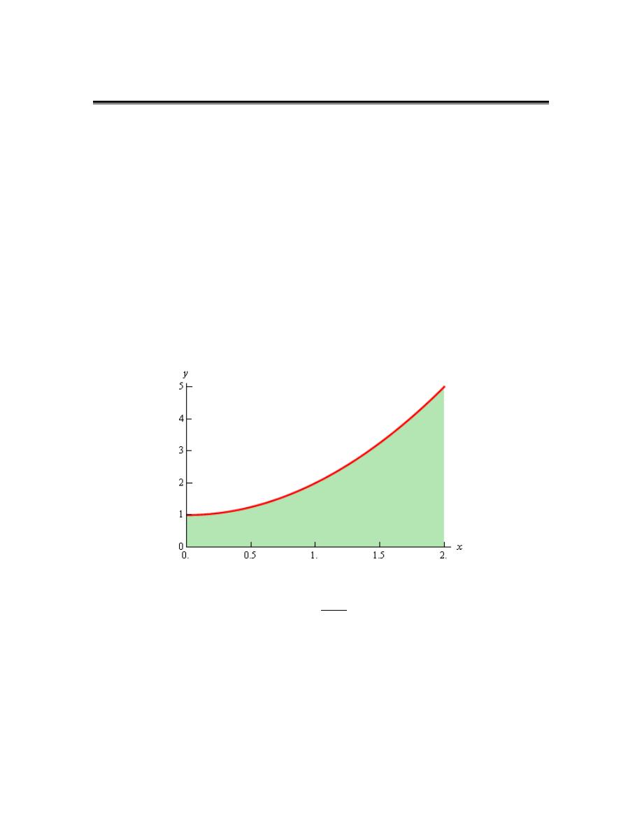
Calculus I
© 2007 Paul Dawkins
46
http://tutorial.math.lamar.edu/terms.aspx
Area Problem
As noted in the first section of this section there are two kinds of integrals and to this point we’ve
looked at indefinite integrals. It is now time to start thinking about the second kind of integral :
Definite Integrals. However, before we do that we’re going to take a look at the Area Problem.
The area problem is to definite integrals what the tangent and rate of change problems are to
derivatives.
The area problem will give us one of the interpretations of a definite integral and it will lead us to
the definition of the definite integral.
To start off we are going to assume that we’ve got a function
( )
f x
that is positive on some
interval [a,b]. What we want to do is determine the area of the region between the function and
the x-axis.
It’s probably easiest to see how we do this with an example. So let’s determine the area between
( )
2
1
f x
x
=
+
on [0,2]. In other words, we want to determine the area of the shaded region
below.
Now, at this point, we can’t do this exactly. However, we can estimate the area. We will
estimate the area by dividing up the interval into n subintervals each of width,
b a
x
n
−
∆ =
Then in each interval we can form a rectangle whose height is given by the function value at a
specific point in the interval. We can then find the area of each of these rectangles, add them up
and this will be an estimate of the area.
It’s probably easier to see this with a sketch of the situation. So, let’s divide up the interval into 4
subintervals and use the function value at the right endpoint of each interval to define the height
of the rectangle. This gives,
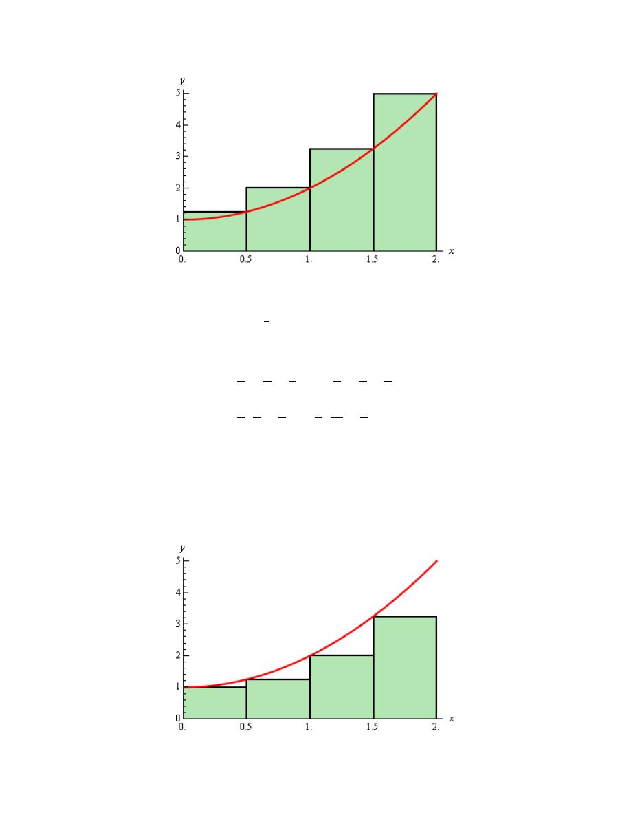
Calculus I
© 2007 Paul Dawkins
47
http://tutorial.math.lamar.edu/terms.aspx
Note that by choosing the height as we did each of the rectangles will over estimate the area since
each rectangle takes in more area than the graph each time. Now let’s estimate the area. First,
the width of each of the rectangles is
1
2
. The height of each rectangle is determined by the
function value at the right endpoint and so the height of each rectangle is nothing more that the
function value at the right endpoint. Here is the estimated area.
( )
( )
( )
( )
1
1
1
1
3
1
1
2
2
2
2
2
2
2
1 5
1
1 13
1
2
5
2 4
2
2
4
2
5.75
r
A
f
f
f
f
=
+
+
+
=
+
+
+
=
Of course taking the rectangle heights to be the function value at the right endpoint is not our only
option. We could have taken the rectangle heights to be the function value at the left endpoint.
Using the left endpoints as the heights of the rectangles will give the following graph and
estimated area.
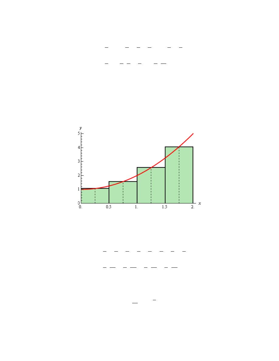
Calculus I
© 2007 Paul Dawkins
48
http://tutorial.math.lamar.edu/terms.aspx
( )
( )
( )
( )
1
1
1
1
1
3
0
1
2
2
2
2
2
2
1
1 5
1
1 13
1
2
2
2 4
2
2
4
3.75
l
A
f
f
f
f
=
+
+
+
=
+
+
+
=
In this case we can see that the estimation will be an underestimation since each rectangle misses
some of the area each time.
There is one more common point for getting the heights of the rectangles that is often more
accurate. Instead of using the right or left endpoints of each sub interval we could take the
midpoint of each subinterval as the height of each rectangle. Here is the graph for this case.
So, it looks like each rectangle will over and under estimate the area. This means that the
approximation this time should be much better than the previous two choices of points. Here is
the estimation for this case.
1
1
1
3
1
5
1
7
2
4
2
4
2
4
2
4
1 17
1 25
1 41
1 65
2 16
2 16
2 16
2 16
4.625
m
A
f
f
f
f
=
+
+
+
=
+
+
+
=
We’ve now got three estimates. For comparison’s sake the exact area is
14
4.666
3
A
=
=
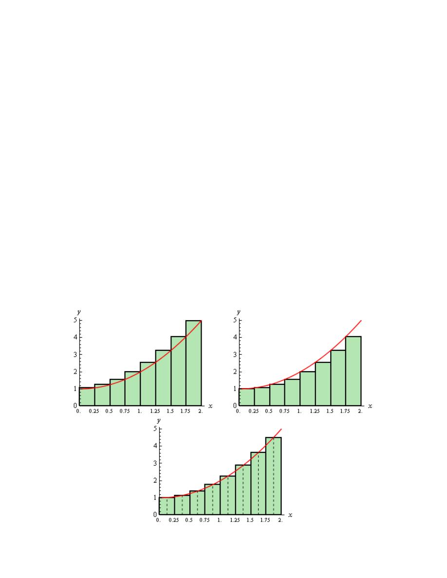
Calculus I
© 2007 Paul Dawkins
49
http://tutorial.math.lamar.edu/terms.aspx
So, both the right and left endpoint estimation did not do all that great of a job at the estimation.
The midpoint estimation however did quite well.
Be careful to not draw any conclusion about how choosing each of the points will affect our
estimation. In this case, because we are working with an increasing function choosing the right
endpoints will overestimate and choosing left endpoint will underestimate.
If we were to work with a decreasing function we would get the opposite results. For decreasing
functions the right endpoints will underestimate and the left endpoints will overestimate.
Also, if we had a function that both increased and decreased in the interval we would, in all
likelihood, not even be able to determine if we would get an overestimation or underestimation.
Now, let’s suppose that we want a better estimation, because none of the estimations above really
did all that great of a job at estimating the area. We could try to find a different point to use for
the height of each rectangle but that would be cumbersome and there wouldn’t be any guarantee
that the estimation would in fact be better. Also, we would like a method for getting better
approximations that would work for any function we would chose to work with and if we just
pick new points that may not work for other functions.
The easiest way to get a better approximation is to take more rectangles (i.e. increase n). Let’s
double the number of rectangles that we used and see what happens. Here are the graphs showing
the eight rectangles and the estimations for each of the three choices for rectangle heights that we
used above.
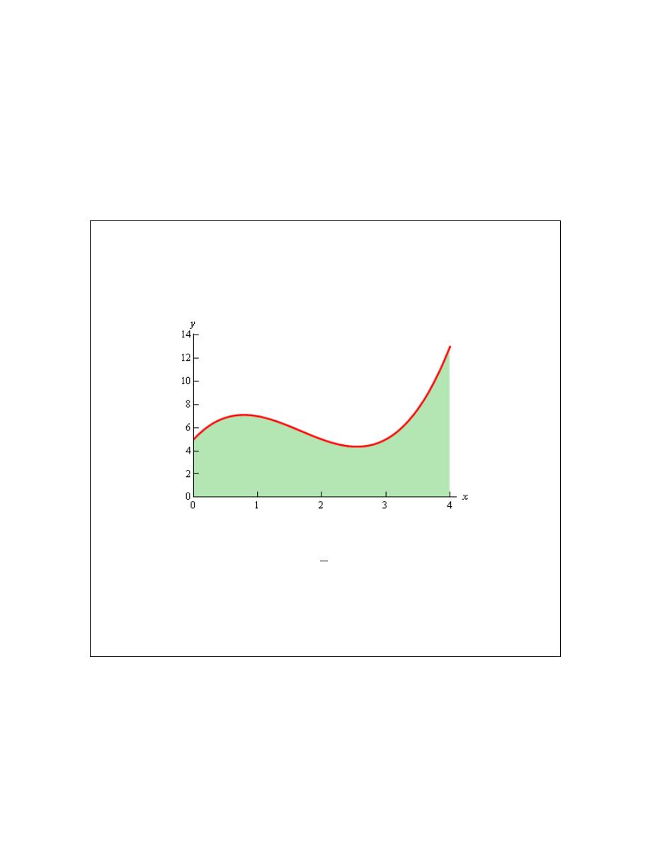
Calculus I
© 2007 Paul Dawkins
50
http://tutorial.math.lamar.edu/terms.aspx
Here are the area estimations for each of these cases.
5.1875
4.1875
4.65625
r
l
m
A
A
A
=
=
=
So, increasing the number of rectangles did improve the accuracy of the estimation as we’d
guessed that it would.
Let’s work a slightly more complicated example.
Example 1
Estimate the area between
( )
3
2
5
6
5
f x
x
x
x
=
−
+
+
and the x-axis using
5
n
=
subintervals and all three cases above for the heights of each rectangle.
Solution
First, let’s get the graph to make sure that the function is positive.
So, the graph is positive and the width of each subinterval will be,
4
0.8
5
x
∆ = =
This means that the endpoints of the subintervals are,
0, 0.8, 1.6, 2.4, 3.2, 4
Let’s first look at using the right endpoints for the function height. Here is the graph for this case.
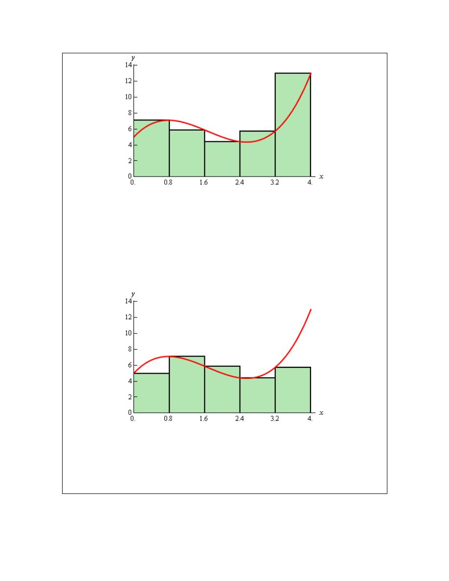
Calculus I
© 2007 Paul Dawkins
51
http://tutorial.math.lamar.edu/terms.aspx
Notice, that unlike the first area we looked at, the choosing the right endpoints here will both over
and underestimate the area depending on where we are on the curve. This will often be the case
with a more general curve that the one we initially looked at. The area estimation using the right
endpoints of each interval for the rectangle height is,
( )
( )
( )
( )
( )
0.8
0.8
0.8
1.6
0.8
2.4
0.8
3.2
0.8
4
28.96
r
A
f
f
f
f
f
=
+
+
+
+
=
Now let’s take a look at left endpoints for the function height. Here is the graph.
The area estimation using the left endpoints of each interval for the rectangle height is,
( )
( )
( )
( )
( )
0.8
0
0.8
0.8
0.8
1.6
0.8
2.4
0.8
3.2
22.56
r
A
f
f
f
f
f
=
+
+
+
+
=
Finally, let’s take a look at the midpoints for the heights of each rectangle. Here is the graph,
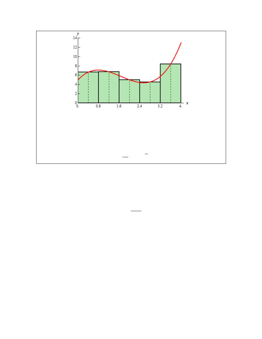
Calculus I
© 2007 Paul Dawkins
52
http://tutorial.math.lamar.edu/terms.aspx
The area estimation using the midpoint is then,
( )
( )
( )
( )
( )
0.8
0.4
0.8
1.2
0.8
2
0.8
2.8
0.8
3.6
25.12
r
A
f
f
f
f
f
=
+
+
+
+
=
For comparison purposes the exact area is,
76
25.333
3
A
=
=
So, again the midpoint did a better job than the other two. While this will be the case more often
than not, it won’t always be the case and so don’t expect this to always happen.
Now, let’s move on to the general case. Let’s start out with
( )
0
f x
≥
on [a,b] and we’ll divide
the interval into n subintervals each of length,
b a
x
n
−
∆ =
Note that the subintervals don’t have to be equal length, but it will make our work significantly
easier. The endpoints of each subinterval are,
(
)
0
1
2
1
2
1
i
n
n
x
a
x
a
x
x
a
x
x
a i x
x
a
n
x
x
a
n x
b
−
=
= + ∆
= + ∆
= + ∆
= +
− ∆
= + ∆ =
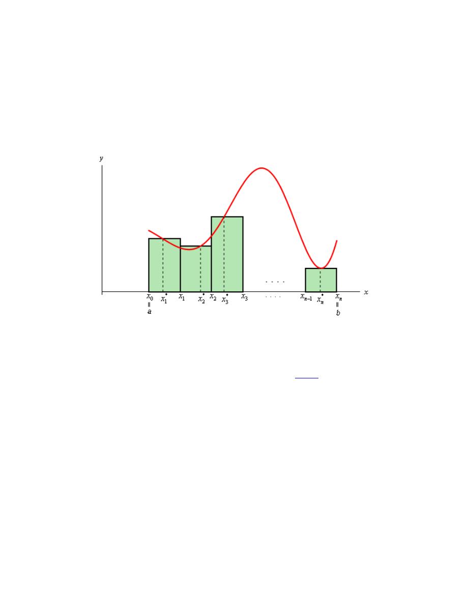
Calculus I
© 2007 Paul Dawkins
53
http://tutorial.math.lamar.edu/terms.aspx
Next in each interval,
[
] [
]
[
]
[
]
0
1
1
2
1
1
,
,
,
,
,
,
,
,
,
i
i
n
n
x x
x x
x
x
x
x
−
−
we choose a point
*
*
*
*
1
2
,
,
,
,
i
n
x x
x
x
. These points will define the height of the rectangle in
each subinterval. Note as well that these points do not have to occur at the same point in each
subinterval.
Here is a sketch of this situation.
The area under the curve on the given interval is then approximately,
( )
( )
( )
( )
*
*
*
*
1
2
i
n
A
f x
x
f x
x
f x
x
f x
x
≈
∆ +
∆ + +
∆ + +
∆
We will use summation notation or sigma notation at this point to simplify up our notation a
little. If you need a refresher on summation notation check out the
section
devoted to this in the
Extras chapter.
Using summation notation the area estimation is,
( )
*
1
n
i
i
A
f x
x
=
≈
∆
∑
The summation in the above equation is called a Riemann Sum.
To get a better estimation we will take n larger and larger. In fact, if we let n go out to infinity we
will get the exact area. In other words,
( )
*
1
lim
n
i
n
i
A
f x
x
→∞
=
=
∆
∑
Before leaving this section let’s address one more issue. To this point we’ve required the
function to be positive in our work. Many functions are not positive however. Consider the case
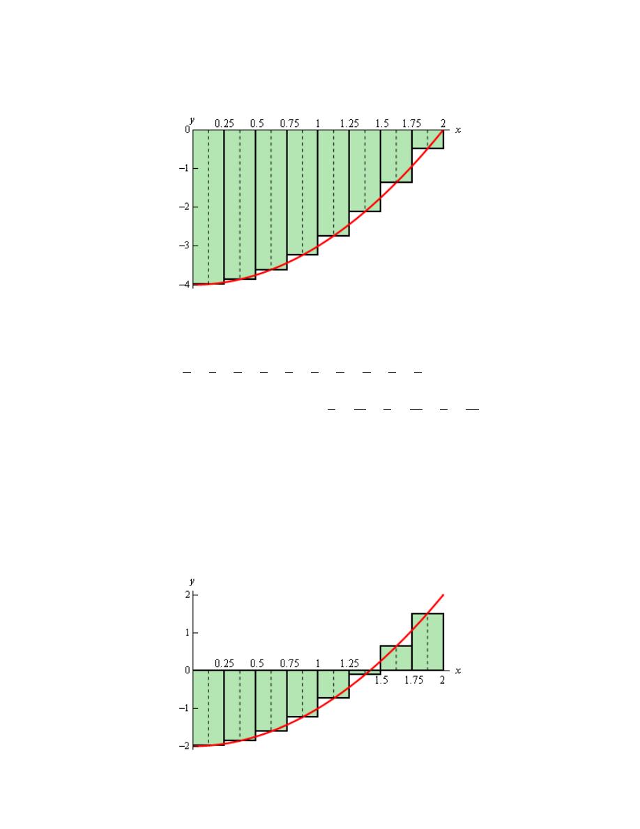
Calculus I
© 2007 Paul Dawkins
54
http://tutorial.math.lamar.edu/terms.aspx
of
( )
2
4
f x
x
=
−
on [0,2]. If we use
8
n
=
and the midpoints for the rectangle height we get the
following graph,
In this case let’s notice that the function lies completely below the x-axis and hence is always
negative. If we ignore the fact that the function is always negative and use the same ideas above
to estimate the area between the graph and the x-axis we get,
1
1
1
3
1
5
1
7
1
9
4
8
4
8
4
8
4
8
4
8
1
11
1
13
1
15
4
8
4
8
4
8
5.34375
m
A
f
f
f
f
f
f
f
f
=
+
+
+
+
+
+
+
= −
Our answer is negative as we might have expected given that all the function evaluations are
negative.
So, using the technique in this section it looks like if the function is above the x-axis we will get a
positive area and if the function is below the x-axis we will get a negative area. Now, what about
a function that is both positive and negative in the interval? For example,
( )
2
2
f x
x
=
−
on
[0,2]. Using
8
n
=
and midpoints the graph is,

Calculus I
© 2007 Paul Dawkins
55
http://tutorial.math.lamar.edu/terms.aspx
Some of the rectangles are below the x-axis and so will give negative areas while some are above
the x-axis and will give positive areas. Since more rectangles are below the x-axis than above it
looks like we should probably get a negative area estimation for this case. In fact that is correct.
Here the area estimation for this case.
1
1
1
3
1
5 1
7
1
9
4
8
4
8
4
8 4
8
4
8
1
11
1
13
1
15
4
8
4
8
4
8
1.34375
m
A
f
f
f
f
f
f
f
f
=
+
+
+
+
+
+
= −
In cases where the function is both above and below the x-axis the technique given in the section
will give the net area between the function and the x-axis with areas below the x-axis negative
and areas above the x-axis positive. So, if the net area is negative then there is more area under
the x-axis than above while a positive net area will mean that more of the area is above the x-axis.

Calculus I
© 2007 Paul Dawkins
56
http://tutorial.math.lamar.edu/terms.aspx
The Definition of the Definite Integral
In this section we will formally define the definite integral and give many of the properties of
definite integrals. Let’s start off with the definition of a definite integral.
Definite Integral
Given a function
( )
f x
that is continuous on the interval [a,b] we divide the interval into n
subintervals of equal width,
x
∆
, and from each interval choose a point,
*
i
x
. Then the definite
integral of f(x) from a to b is
( )
( )
*
1
lim
n
b
i
a
n
i
f x dx
f x
x
→∞
=
=
∆
∑
∫
The definite integral is defined to be exactly the limit and summation that we looked at in the last
section to find the net area between a function and the x-axis. Also note that the notation for the
definite integral is very similar to the notation for an indefinite integral. The reason for this will
be apparent eventually.
There is also a little bit of terminology that we should get out of the way here. The number “a”
that is at the bottom of the integral sign is called the lower limit of the integral and the number
“b” at the top of the integral sign is called the upper limit of the integral. Also, despite the fact
that a and b were given as an interval the lower limit does not necessarily need to be smaller than
the upper limit. Collectively we’ll often call a and b the interval of integration.
Let’s work a quick example. This example will use many of the properties and facts from the
brief review of
summation notation
in the Extras chapter.
Example 1
Using the definition of the definite integral compute the following.
2
2
0
1
x
dx
+
∫
Solution
First, we can’t actually use the definition unless we determine which points in each interval that
well use for
*
i
x
. In order to make our life easier we’ll use the right endpoints of each interval.
From the previous section we know that for a general n the width of each subinterval is,
2 0
2
x
n
n
−
∆ =
=
The subintervals are then,
( )
(
)
2
1
2
1
2
2 4
4 6
2
0,
,
,
,
,
,
,
,
,
,
, 2
i
n
i
n
n n
n n
n
n
n
−
−
As we can see the right endpoint of the i
th
subinterval is

Calculus I
© 2007 Paul Dawkins
57
http://tutorial.math.lamar.edu/terms.aspx
*
2
i
i
x
n
=
The summation in the definition of the definite integral is then,
( )
*
1
1
2
1
2
3
1
2
2
2
2
1
8
2
n
n
i
i
i
n
i
n
i
i
f x
x
f
n
n
i
n
n
i
n
n
=
=
=
=
∆ =
=
+
=
+
∑
∑
∑
∑
Now, we are going to have to take a limit of this. That means that we are going to need to
“evaluate” this summation. In other words, we are going to have to use the formulas given in the
summation notation
review to eliminate the actual summation and get a formula for this for a
general n.
To do this we will need to recognize that n is a constant as far as the summation notation is
concerned. As we cycle through the integers from 1 to n in the summation only i changes and so
anything that isn’t an i will be a constant and can be factored out of the summation. In particular
any n that is in the summation can be factored out if we need to.
Here is the summation “evaluation”.
( )
(
)(
)
( )
(
)(
)
2
*
3
1
1
1
2
3
1
1
3
2
2
2
8
2
8
1
2
1 2
1
8
1
2
6
4
1 2
1
2
3
14
12
4
3
n
n
n
i
i
i
i
n
n
i
i
i
f x
x
n
n
i
n
n
n n
n
n
n
n
n
n
n
n
n
n
=
=
=
=
=
∆ =
+
=
+
+
+
=
+
+
+
=
+
+
+
=
∑
∑
∑
∑
∑
We can now compute the definite integral.

Calculus I
© 2007 Paul Dawkins
58
http://tutorial.math.lamar.edu/terms.aspx
( )
2
2
*
0
1
2
2
1
lim
14
12
4
lim
3
14
3
n
i
n
i
n
x
dx
f x
x
n
n
n
→∞
=
→∞
+
=
∆
+
+
=
=
∑
∫
We’ve seen several methods for dealing with the limit in this problem so I’ll leave it to you to
verify the results.
Wow, that was a lot of work for a fairly simple function. There is a much simpler way of
evaluating these and we will get to it eventually. The main purpose to this section is to get the
main properties and facts about the definite integral out of the way. We’ll discuss how we
compute these in practice starting with the next section.
So, let’s start taking a look at some of the properties of the definite integral.
Properties
1.
( )
( )
b
a
a
b
f x dx
f x dx
= −
∫
∫
. We can interchange the limits on any definite integral, all that
we need to do is tack a minus sign onto the integral when we do.
2.
( )
0
a
a
f x dx
=
∫
. If the upper and lower limits are the same then there is no work to do, the
integral is zero.
3.
( )
( )
b
b
a
a
cf x dx
c
f x dx
=
∫
∫
, where c is any number. So, as with limits, derivatives, and
indefinite integrals we can factor out a constant.
4.
( )
( )
( )
( )
b
b
b
a
a
a
f x
g x dx
f x dx
g x dx
±
=
±
∫
∫
∫
. We can break up definite integrals across a
sum or difference.
5.
( )
( )
( )
b
c
b
a
a
c
f x dx
f x dx
f x dx
=
+
∫
∫
∫
where c is any number. This property is more
important than we might realize at first. One of the main uses of this property is to tell us
how we can integrate a function over the adjacent intervals, [a,c] and [c,b]. Note however
that c doesn’t need to be between a and b.
6.
( )
( )
b
b
a
a
f x dx
f t dt
=
∫
∫
. The point of this property is to notice that as long as the function
and limits are the same the variable of integration that we use in the definite integral won’t
affect the answer.

Calculus I
© 2007 Paul Dawkins
59
http://tutorial.math.lamar.edu/terms.aspx
See the
Proof of Various Integral Properties
section of the Extras chapter for the proof of
properties 1 – 4. Property 5 is not easy to prove and so is not shown there. Property 6 is not
really a property in the full sense of the word. It is only here to acknowledge that as long as the
function and limits are the same it doesn’t matter what letter we use for the variable. The answer
will be the same.
Let’s do a couple of examples dealing with these properties.
Example 2
Use the results from the first example to evaluate each of the following.
(a)
0
2
2
1
x
dx
+
∫
[
Solution
]
(b)
2
2
0
10
10
x
dx
+
∫
[
Solution
]
(c)
2
2
0
1
t
dt
+
∫
[
Solution
]
Solution
All of the solutions to these problems will rely on the fact we proved in the first example.
Namely that,
2
2
0
14
1
3
x
dx
+
=
∫
(a)
0
2
2
1
x
dx
+
∫
In this case the only difference between the two is that the limits have interchanged. So, using the
first property gives,
0
2
2
2
2
0
1
1
14
3
x
dx
x
dx
+
= −
+
= −
∫
∫
[
Return to Problems
]
(b)
2
2
0
10
10
x
dx
+
∫
For this part notice that we can factor a 10 out of both terms and then out of the integral using the
third property.
(
)
2
2
2
2
0
0
2
2
0
10
10
10
1
10
1
14
10
3
140
3
x
dx
x
dx
x
dx
+
=
+
=
+
=
=
∫
∫
∫
[
Return to Problems
]

Calculus I
© 2007 Paul Dawkins
60
http://tutorial.math.lamar.edu/terms.aspx
(c)
2
2
0
1
t
dt
+
∫
In this case the only difference is the letter used and so this is just going to use property 6.
2
2
2
2
0
0
14
1
1
3
t
dt
x
dx
+
=
+
=
∫
∫
[
Return to Problems
]
Here are a couple of examples using the other properties.
Example 3
Evaluate the following definite integral.
( )
( )
130
3
2
130
sin
cos
1
x
x
x
x
dx
x
−
+
+
⌠
⌡
Solution
There really isn’t anything to do with this integral once we notice that the limits are the same.
Using the second property this is,
( )
( )
130
3
2
130
sin
cos
0
1
x
x
x
x
dx
x
−
+
=
+
⌠
⌡
Example 4
Given that
( )
10
6
23
f x dx
−
=
∫
and
( )
6
10
9
g x dx
−
= −
∫
determine the value of
( )
( )
6
10
2
10
f x
g x dx
−
−
∫
Solution
We will first need to use the fourth property to break up the integral and the third property to
factor out the constants.
( )
( )
( )
( )
( )
( )
6
6
6
10
10
10
6
6
10
10
2
10
2
10
2
10
f x
g x dx
f x dx
g x dx
f x dx
g x dx
−
−
−
−
−
−
=
−
=
−
∫
∫
∫
∫
∫
Now notice that the limits on the first integral are interchanged with the limits on the given
integral so switch them using the first property above (and adding a minus sign of course). Once
this is done we can plug in the known values of the integrals.
( )
( )
( )
( )
( )
( )
6
10
6
10
6
10
2
10
2
10
2 23
10
9
44
f x
g x dx
f x dx
g x dx
−
−
−
−
= −
−
= −
−
−
=
∫
∫
∫

Calculus I
© 2007 Paul Dawkins
61
http://tutorial.math.lamar.edu/terms.aspx
Example 5
Given that
( )
10
12
6
f x dx
−
=
∫
,
( )
10
100
2
f x dx
−
= −
∫
, and
( )
5
100
4
f x dx
−
=
∫
determine
the value of
( )
12
5
f x dx
−
∫
.
Solution
This example is mostly an example of property 5 although there are a couple of uses of property 1
in the solution as well.
We need to figure out how to correctly break up the integral using property 5 to allow us to use
the given pieces of information. First we’ll note that there is an integral that has a “-5” in one of
the limits. It’s not the lower limit, but we can use property 1 to correct that eventually. The other
limit is 100 so this is the number c that we’ll use in property 5.
( )
( )
( )
12
100
12
5
5
100
f x dx
f x dx
f x dx
−
−
=
+
∫
∫
∫
We’ll be able to get the value of the first integral, but the second still isn’t in the list of know
integrals. However, we do have second limit that has a limit of 100 in it. The other limit for this
second integral is -10 and this will be c in this application of property 5.
( )
( )
( )
( )
12
100
10
12
5
5
100
10
f x dx
f x dx
f x dx
f x dx
−
−
−
−
=
+
+
∫
∫
∫
∫
At this point all that we need to do is use the property 1 on the first and third integral to get the
limits to match up with the known integrals. After that we can plug in for the known integrals.
( )
( )
( )
( )
12
5
10
10
5
100
100
12
4 2 6
12
f x dx
f x dx
f x dx
f x dx
−
−
−
−
= −
+
−
= − − −
= −
∫
∫
∫
∫
There are also some nice properties that we can use in comparing the general size of definite
integrals. Here they are.
More Properties
7.
(
)
b
a
c dx
c b a
=
−
∫
, c is any number.
8. If
( )
0
f x
≥
for
a
x
b
≤ ≤
then
( )
0
b
a
f x dx
≥
∫
.
9. If
( )
( )
f x
g x
≥
for
a
x
b
≤ ≤
then
( )
( )
b
b
a
a
f x dx
g x dx
≥
∫
∫
.
10. If
( )
m
f x
M
≤
≤
for
a
x
b
≤ ≤
then
(
)
( )
(
)
b
a
m b a
f x dx
M b a
−
≤
≤
−
∫
.
11.
( )
( )
b
b
a
a
f x dx
f x dx
≤
∫
∫

Calculus I
© 2007 Paul Dawkins
62
http://tutorial.math.lamar.edu/terms.aspx
See the
Proof of Various Integral Properties
section of the Extras chapter for the proof of these
properties.
Interpretations of Definite Integral
There are a couple of quick interpretations of the definite integral that we can give here.
First, as we alluded to in the previous section one possible interpretation of the definite integral is
to give the net area between the graph of
( )
f x
and the x-axis on the interval [a,b]. So, the net
area between the graph of
( )
2
1
f x
x
=
+
and the x-axis on [0,2] is,
2
2
0
14
1
3
x
dx
+
=
∫
If you look back in the last section this was the exact area that was given for the initial set of
problems that we looked at in this area.
Another interpretation is sometimes called the Net Change Theorem. This interpretation says that
if
( )
f x
is some quantity (so
( )
f
x
′
is the rate of change of
( )
f x
, then,
( )
( )
( )
b
a
f
x dx
f b
f a
′
=
−
∫
is the net change in
( )
f x
on the interval [a,b]. In other words, compute the definite integral of
a rate of change and you’ll get the net change in the quantity. We can see that the value of the
definite integral,
( )
( )
f b
f a
−
, does in fact give use the net change in
( )
f x
and so there really
isn’t anything to prove with this statement. This is really just an acknowledgment of what the
definite integral of a rate of change tells us.
So as a quick example, if
( )
V t
is the volume of water in a tank then,
( )
( )
( )
2
1
2
1
t
t
V t dt
V t
V t
′
=
−
∫
is the net change in the volume as we go from time
1
t
to time
2
t
.
Likewise, if
( )
s t
is the function giving the position of some object at time t we know that the
velocity of the object at any time t is :
( )
( )
v t
s t
′
=
. Therefore the displacement of the object
time
1
t
to time
2
t
is,
( )
( ) ( )
2
1
2
1
t
t
v t dt
s t
s t
=
−
∫
Note that in this case if
( )
v t
is both positive and negative (i.e. the object moves to both the right
and left) in the time frame this will NOT give the total distance traveled. It will only give the
displacement, i.e. the difference between where the object started and where it ended up. To get
the total distance traveled by an object we’d have to compute,

Calculus I
© 2007 Paul Dawkins
63
http://tutorial.math.lamar.edu/terms.aspx
( )
2
1
t
t
v t dt
∫
It is important to note here that the Net Change Theorem only really makes sense if we’re
integrating a derivative of a function.
Fundamental Theorem of Calculus, Part I
As noted by the title above this is only the first part to the Fundamental Theorem of Calculus.
We will give the second part in the next section as it is the key to easily computing definite
integrals and that is the subject of the next section.
The first part of the Fundamental Theorem of Calculus tells us how to differentiate certain types
of definite integrals and it also tells us about the very close relationship between integrals and
derivatives.
Fundamental Theorem of Calculus, Part I
If
( )
f x
is continuous on [a,b] then,
( )
( )
x
a
g x
f t dt
=
∫
is continuous on [a,b] and it is differentiable on
( )
,
a b
and that,
( )
( )
g x
f x
′
=
An alternate notation for the derivative portion of this is,
( )
( )
x
a
d
f t dt
f x
dx
=
∫
To see the proof of this see the
Proof of Various Integral Properties
section of the Extras chapter.
Let’s check out a couple of quick examples using this.
Example 6
Differentiate each of the following.
(a)
( )
(
)
2
2
4
cos 1 5
x
t
g x
t dt
−
=
−
∫
e
[
Solution
]
(b)
2
1
4
2
1
1
x
t
dt
t
+
+
⌠
⌡
[
Solution
]
Solution
(a)
( )
(
)
2
2
4
cos 1 5
x
t
g x
t dt
−
=
−
∫
e
This one is nothing more than a quick application of the Fundamental Theorem of Calculus.
( )
(
)
2
2
cos 1 5
x
g x
x
′
=
−
e
[
Return to Problems
]

Calculus I
© 2007 Paul Dawkins
64
http://tutorial.math.lamar.edu/terms.aspx
(b)
2
1
4
2
1
1
x
t
dt
t
+
+
⌠
⌡
This one needs a little work before we can use the Fundamental Theorem of Calculus. The first
thing to notice is that the FToC requires the lower limit to be a constant and the upper limit to be
the variable. So, using a property of definite integrals we can interchange the limits of the
integral we just need to remember to add in a minus sign after we do that. Doing this gives,
2
2
2
1
4
4
4
2
2
2
1
1
1
1
1
1
1
1
x
x
x
d
t
d
t
d
t
dt
dt
dt
dx
t
dx
t
dx
t
+
+
+
=
−
= −
+
+
+
⌠
⌠
⌠
⌡
⌡
⌡
The next thing to notice is that the FToC also requires an x in the upper limit of integration and
we’ve got x
2
. To do this derivative we’re going to need the following version of the
chain rule
.
( )
(
)
( )
(
)
( )
where
d
d
du
g u
g u
u
f x
dx
du
dx
=
=
So, if we let u= x
2
we use the chain rule to get,
( )
2
2
1
4
4
2
2
1
4
2
2
1
4
2
4
2
1
1
1
1
1
where
1
1
2
1
1
2
1
x
x
u
d
t
d
t
dt
dt
dx
t
dx
t
d
t
du
dt
u
x
du
t
dx
u
x
u
u
x
u
+
+
= −
+
+
+
= −
=
+
+
= −
+
+
= −
+
⌠
⌠
⌡
⌡
⌠
⌡
The final step is to get everything back in terms of x.
( )
( )
2
4
2
1
4
2
2
2
8
4
1
1
2
1
1
1
2
1
x
x
d
t
dt
x
dx
t
x
x
x
x
+
+
= −
+
+
+
= −
+
⌠
⌡
[
Return to Problems
]
Using the chain rule as we did in the last part of this example we can derive some general
formulas for some more complicated problems.
First,
( )
( )
( )
( )
(
)
u x
a
d
f t dt
u x f u x
dx
′
=
∫
This is simply the chain rule for these kinds of problems.

Calculus I
© 2007 Paul Dawkins
65
http://tutorial.math.lamar.edu/terms.aspx
Next, we can get a formula for integrals in which the upper limit is a constant and the lower limit
is a function of x. All we need to do here is interchange the limits on the integral (adding in a
minus sign of course) and then using the formula above to get,
( )
( )
( )
( )
( )
( )
(
)
b
v x
v x
b
d
d
f t dt
f t dt
v x f v x
dx
dx
′
= −
= −
∫
∫
Finally, we can also get a version for both limits being functions of x. In this case we’ll need to
use Property 5 above to break up the integral as follows,
( )
( )
( )
( )
( )
( )
( )
u x
a
u x
v x
v x
a
f t dt
f t dt
f t dt
=
+
∫
∫
∫
We can use pretty much any value of a when we break up the integral. The only thing that we
need to avoid is to make sure that
( )
f a
exists. So, assuming that
( )
f a
exists after we break
up the integral we can then differentiate and use the two formulas above to get,
( )
( )
( )
( )
( )
( )
( )
(
)
( )
( )
(
)
( )
( )
(
)
u x
a
u x
v x
v x
a
d
d
f t dt
f t dt
f t dt
dx
dx
v x f v x
u x f u x
=
+
′
′
= −
+
∫
∫
∫
Let’s work a quick example.
Example 7
Differentiate the following integral.
(
)
3
2
2
sin 1
x
x
t
t
dt
+
∫
Solution
This will use the final formula that we derived above.
(
)
( )
( )
(
)
( )( )
( )
(
)
(
)
(
)
1
2
2
3
2
2
2
2
2
2
2
1
sin 1
sin 1
3 3
sin 1
3
2
1
sin 1
27
sin 1 9
2
x
x
d
t
t
dt
x
x
x
x
x
dx
x
x
x
x
−
+
= −
+
+
+
= −
+
+
+
∫

Calculus I
© 2007 Paul Dawkins
66
http://tutorial.math.lamar.edu/terms.aspx
Computing Definite Integrals
In this section we are going to concentrate on how we actually evaluate definite integrals in
practice. To do this we will need the Fundamental Theorem of Calculus, Part II.
Fundamental Theorem of Calculus, Part II
Suppose
( )
f x
is a continuous function on [a,b] and also suppose that
( )
F x
is any anti-
derivative for
( )
f x
. Then,
( )
( )
( )
( )
b
b
a
a
f x dx
F x
F b
F a
=
=
−
∫
To see the proof of this see the
Proof of Various Integral Properties
section of the Extras chapter.
Recall that when we talk about an anti-derivative for a function we are really talking about the
indefinite integral for the function. So, to evaluate a definite integral the first thing that we’re
going to do is evaluate the indefinite integral for the function. This should explain the similarity
in the notations for the indefinite and definite integrals.
Also notice that we require the function to be continuous in the interval of integration. This was
also a requirement in the definition of the definite integral. We didn’t make a big deal about this
in the last section. In this section however, we will need to keep this condition in mind as we do
our evaluations.
Next let’s address the fact that we can use any anti-derivative of
( )
f x
in the evaluation. Let’s
take a final look at the following integral.
2
2
0
1
x
dx
+
∫
Both of the following are anti-derivatives of the integrand.
( )
( )
3
3
1
1
18
and
3
3
31
F x
x
x
F x
x
x
=
+
=
+ −
Using the FToC to evaluate this integral with the first anti-derivatives gives,
( )
( )
2
2
2
3
0
0
3
3
1
1
3
1
1
2
2
0
0
3
3
14
3
x
dx
x
x
+
=
+
=
+ −
+
=
∫

Calculus I
© 2007 Paul Dawkins
67
http://tutorial.math.lamar.edu/terms.aspx
Much easier than
using the definition
wasn’t it? Let’s now use the second anti-derivative to
evaluate this definite integral.
( )
( )
2
2
2
3
0
0
3
3
1
18
1
3
31
1
18
1
18
2
2
0
0
3
31
3
31
14
18
18
3
31
31
14
3
x
dx
x
x
+
=
+ −
=
+ −
−
+ −
=
−
+
=
∫
The constant that we tacked onto the second anti-derivative canceled in the evaluation step. So,
when choosing the anti-derivative to use in the evaluation process make your life easier and don’t
bother with the constant as it will only end up canceling in the long run.
Also, note that we’re going to have to be very careful with minus signs and parenthesis with these
problems. It’s very easy to get in a hurry and mess them up.
Let’s start our examples with the following set designed to make a couple of quick points that are
very important.
Example 1
Evaluate each of the following.
(a)
2
2
y
y
dy
−
+
∫
[
Solution
]
(b)
2
2
2
1
y
y
dy
−
+
∫
[
Solution
]
(c)
2
2
2
1
y
y
dy
−
−
+
∫
[
Solution
]
Solution
(a)
2
2
y
y
dy
−
+
∫
This is the only indefinite integral in this section and by now we should be getting pretty good
with these so we won’t spend a lot of time on this part. This is here only to make sure that we
understand the difference between an indefinite and a definite integral. The integral is,
2
2
3
1
1
3
y
y
dy
y
y
c
−
−
+
=
−
+
∫
[
Return to Problems
]
(b)
2
2
2
1
y
y
dy
−
+
∫
Recall from our first example above that all we really need here is any anti-derivative of the
integrand. We just computed the most general anti-derivative in the first part so we can use that
if we want to. However, recall that as we noted above any constants we tack on will just cancel

Calculus I
© 2007 Paul Dawkins
68
http://tutorial.math.lamar.edu/terms.aspx
in the long run and so we’ll use the answer from (a) without the “+c”.
Here’s the integral,
( )
( )
2
2
2
2
3
1
1
3
3
1
1
3
1
1
1
1
2
1
3
2
3
1
8
1
1
1
3
2
3
17
6
y
y
dy
y
y
−
+
=
−
=
− −
−
= − − +
=
∫
Remember that the evaluation is always done in the order of evaluation at the upper limit minus
evaluation at the lower limit. Also be very careful with minus signs and parenthesis. It’s very
easy to forget them or mishandle them and get the wrong answer.
Notice as well that, in order to help with the evaluation, we rewrote the indefinite integral a little.
In particular we got rid of the negative exponent on the second term. It’s generally easier to
evaluate the term with positive exponents.
[
Return to Problems
]
(c)
2
2
2
1
y
y
dy
−
−
+
∫
This integral is here to make a point. Recall that in order for us to do an integral the integrand
must be continuous in the range of the limits. In this case the second term will have division by
zero at
0
y
=
and since
0
y
=
is in the interval of integration, i.e. it is between the lower and
upper limit, this integrand is not continuous in the interval of integration and so we can’t do this
integral.
Note that this problem will not prevent us from doing the integral in (b) since
0
y
=
is not in the
interval of integration.
[
Return to Problems
]
So what have we learned from this example?
First, in order to do a definite integral the first thing that we need to do is the indefinite integral.
So we aren’t going to get out of doing indefinite integrals, they will be in every integral that we’ll
be doing in the rest of this course so make sure that you’re getting good at computing them.
Second, we need to be on the lookout for functions that aren’t continuous at any point between
the limits of integration. Also, it’s important to note that this will only be a problem if the

Calculus I
© 2007 Paul Dawkins
69
http://tutorial.math.lamar.edu/terms.aspx
point(s) of discontinuity occur between the limits of integration or at the limits themselves. If the
point of discontinuity occurs outside of the limits of integration the integral can still be evaluated.
In the following sets of examples we won’t make too much of an issue with continuity problems,
or lack of continuity problems, unless it affects the evaluation of the integral. Do not let this
convince you that you don’t need to worry about this idea. It arises often enough that it can cause
real problems if you aren’t on the lookout for it.
Finally, note the difference between indefinite and definite integrals. Indefinite integrals are
functions while definite integrals are numbers.
Let’s work some more examples.
Example 2
Evaluate each of the following.
(a)
1
2
3
6
5
2
x
x
dx
−
−
+
∫
[
Solution
]
(b)
(
)
0
4
2
t t
dt
−
∫
[
Solution
]
(c)
2
5
2
1
2
3
w
w
dw
w
− +
⌠
⌡
[
Solution
]
(d)
10
25
dR
−
∫
[
Solution
]
Solution
(a)
1
2
3
6
5
2
x
x
dx
−
−
+
∫
There isn’t a lot to this one other than simply doing the work.
1
1
2
3
2
3
3
5
6
5
2
2
2
2
5
45
2
2
54
6
2
2
84
x
x
dx
x
x
x
−
−
−
+
=
−
+
=
− +
− − −
−
=
∫
[
Return to Problems
]
(b)
(
)
0
4
2
t t
dt
−
∫
Recall that we can’t integrate products as a product of integrals and so we first need to multiply
the integrand out before integrating, just as we did in the indefinite integral case.

Calculus I
© 2007 Paul Dawkins
70
http://tutorial.math.lamar.edu/terms.aspx
(
)
( )
( )
3
1
0
0
2
2
4
4
0
5
3
2
2
4
5
3
2
2
2
2
2
4
5
3
2
4
0
4
4
5
3
32
15
t t
dt
t
t dt
t
t
−
=
−
=
−
= −
−
= −
∫
∫
In the evaluation process recall that,
( )
( )
( )
5
5
1
5
2
2
4
4
2
32
=
=
=
( )
( )
( )
3
3
1
3
2
2
4
4
2
8
=
=
=
Also, don’t get excited about the fact that the lower limit of integration is larger than the upper
limit of integration. That will happen on occasion and there is absolutely nothing wrong with
this.
[
Return to Problems
]
(c)
2
5
2
1
2
3
w
w
dw
w
− +
⌠
⌡
First, notice that we will have a division by zero issue at
0
w
=
, but since this isn’t in the interval
of integration we won’t have to worry about it.
Next again recall that we can’t integrate quotients as a quotient of integrals and so the first step
that we’ll need to do is break up the quotient so we can integrate the function.
2
2
5
3
2
2
1
1
2
4
1
2
3
1
2
3
1
3
ln
2
3
1
8 ln 2
ln1 3
2
2
9 ln 2
w
w
dw
w
w dw
w
w
w
w
w
−
− +
=
− +
=
−
−
=
−
−
−
−
−
= −
⌠
⌠
⌡
⌡
Don’t get excited about answers that don’t come down to a simple integer or fraction. Often
times they won’t. Also don’t forget that
( )
ln 1
0
=
.
[
Return to Problems
]

Calculus I
© 2007 Paul Dawkins
71
http://tutorial.math.lamar.edu/terms.aspx
(d)
10
25
dR
−
∫
This one is actually pretty easy. Recall that we’re just integrating 1!.
10
10
25
25
10 25
35
dR
R
−
−
=
= − −
= −
∫
[
Return to Problems
]
The last set of examples dealt exclusively with integrating powers of x. Let’s work a couple of
examples that involve other functions.
Example 3
Evaluate each of the following.
(a)
1
3
2
0
4
6
x
x dx
−
∫
[
Solution
]
(b)
3
0
2 sin
5 cos d
π
θ
θ θ
−
∫
[
Solution
]
(c)
4
6
5 2 sec tan
z
z dz
π
π
−
∫
[
Solution
]
(d)
1
20
3
1
3
z
dz
z
−
−
−
−
⌠
⌡ e
[
Solution
]
(e)
3
6
2
1
5
10
t
t
dt
t
−
−
+
⌠
⌡
[
Solution
]
Solution
(a)
1
3
2
0
4
6
x
x dx
−
∫
.
This one is here mostly here to contrast with the next example.
( )
2
1
1
3
2
3
0
0
1
5
2
3
0
4
6
4
6
18
2
5
18
2
0
5
8
5
x
x dx
x
x dx
x
x
−
=
−
=
−
= −
−
= −
∫
∫
[
Return to Problems
]
(b)
3
0
2 sin
5 cos d
π
θ
θ θ
−
∫
Be careful with signs with this one. Recall from the indefinite integral sections that it’s easy to
mess up the signs when integrating sine and cosine.

Calculus I
© 2007 Paul Dawkins
72
http://tutorial.math.lamar.edu/terms.aspx
(
)
(
)
3
3
0
0
2 sin
5 cos
2 cos
5sin
2 cos
5sin
2 cos 0 5sin 0
3
3
5 3
1
2
2
5 3
1
2
d
π
π
θ
θ θ
θ
θ
π
π
−
= −
−
= −
−
− −
−
= − −
+
= −
∫
Compare this answer to the previous answer, especially the evaluation at zero. It’s very easy to
get into the habit of just writing down zero when evaluating a function at zero. This is especially
a problem when many of the functions that we integrate involve only x’s raised to positive
integers; these evaluate is zero of course. After evaluating many of these kinds of definite
integrals it’s easy to get into the habit of just writing down zero when you evaluate at zero.
However, there are many functions out there that aren’t zero when evaluated at zero so be careful.
[
Return to Problems
]
(c)
4
6
5 2 sec tan
z
z dz
π
π
−
∫
Not much to do other than do the integral.
(
)
4
4
6
6
5 2 sec tan
5
2 sec
5
2 sec
5
2 sec
4
4
6
6
5
4
2 2
12
3
z
z dz
z
z
π
π
π
π
π
π
π
π
π
−
=
−
=
−
−
−
=
−
+
∫
For the evaluation, recall that
1
sec
cos
z
z
=
and so if we can evaluate cosine at these angles we can evaluate secant at these angles.
[
Return to Problems
]
(d)
1
20
3
1
3
z
dz
z
−
−
−
−
⌠
⌡ e
In order to do this one will need to rewrite both of the terms in the integral a little as follows,
1
1
20
20
3
1
1 1
3
3
3
z
z
dz
dz
z
z
−
−
−
−
−
−
=
−
⌠
⌠
⌡
⌡
e
e
For the first term recall we used the following fact about exponents.
1
1
a
a
a
a
x
x
x
x
−
−
=
=

Calculus I
© 2007 Paul Dawkins
73
http://tutorial.math.lamar.edu/terms.aspx
In the second term, taking the 3 out of the denominator will just make integrating that term easier.
Now the integral.
1
1
20
20
1
20
1
20
3
1
1
3
ln
3
3
1
1
3
ln 1
3
ln 20
3
3
1
3
3
ln 20
3
z
z
dz
z
z
−
−
−
−
−
−
−
−
−
−
=
−
=
−
− −
−
−
=
−
+
⌠
⌡
e
e
e
e
e
e
Just leave the answer like this. It’s messy, but it’s also exact.
Note that the absolute value bars on the logarithm are required here. Without them we couldn’t
have done the evaluation.
[
Return to Problems
]
(e)
3
6
2
1
5
10
t
t
dt
t
−
−
+
⌠
⌡
This integral can’t be done. There is division by zero in the third term at
0
t
=
and
0
t
=
lies in
the interval of integration. The fact that the first two terms can be integrated doesn’t matter. If
even one term in the integral can’t be integrated then the whole integral can’t be done.
[
Return to Problems
]
So, we’ve computed a fair number of definite integrals at this point. Remember that the vast
majority of the work in computing them is first finding the indefinite integral. Once we’ve found
that the rest is just some number crunching.
There are a couple of particularly tricky definite integrals that we need to take a look at next.
Actually they are only tricky until you see how to do them, so don’t get too excited about them.
The first one involves integrating a piecewise function.
Example 4
Given,
( )
2
6
if 1
3
if 1
x
f x
x
x
>
=
≤
Evaluate each of the following integrals.
(a)
( )
22
10
f x dx
∫
[
Solution
]
(b)
( )
3
2
f x dx
−
∫
[
Solution
]
Solution
Let’s first start with a graph of this function.
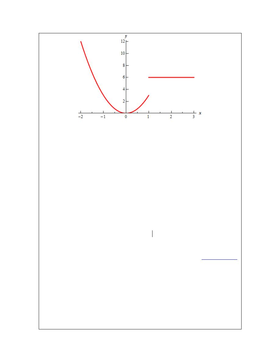
Calculus I
© 2007 Paul Dawkins
74
http://tutorial.math.lamar.edu/terms.aspx
The graph reveals a problem. This function is not continuous at
1
x
=
and we’re going to have to
watch out for that.
(a)
( )
22
10
f x dx
∫
For this integral notice that
1
x
=
is not in the interval of integration and so that is something that
we’ll not need to worry about in this part.
Also note the limits for the integral lie entirely in the range for the first function. What this
means for us is that when we do the integral all we need to do is plug in the first function into the
integral.
Here is the integral.
( )
22
22
10
10
22
10
6
6
132 60
72
f x dx
dx
x
=
=
=
−
=
∫
∫
[
Return to Problems
]
(b)
( )
3
2
f x dx
−
∫
In this part
1
x
=
is between the limits of integration. This means that the integrand is no longer
continuous in the interval of integration and that is a show stopper as far we’re concerned. As
noted above we simply can’t integrate functions that aren’t continuous in the interval of
integration.
Also, even if the function was continuous at
1
x
=
we would still have the problem that the
function is actually two different equations depending where we are in the interval of integration.

Calculus I
© 2007 Paul Dawkins
75
http://tutorial.math.lamar.edu/terms.aspx
Let’s first address the problem of the function not being continuous at
1
x
=
. As we’ll see, in this
case, if we can find a way around this problem the second problem will also get taken care of at
the same time.
In the previous examples where we had functions that weren’t continuous we had division by
zero and no matter how hard we try we can’t get rid of that problem. Division by zero is a real
problem and we can’t really avoid it. In this case the discontinuity does not stem from problems
with the function not existing at
1
x
=
. Instead the function is not continuous because it takes on
different values on either sides of
1
x
=
. We can “remove” this problem by recalling
Property 5
from the previous section. This property tells us that we can write the integral as follows,
( )
( )
( )
3
1
3
2
2
1
f x dx
f x dx
f x dx
−
−
=
+
∫
∫
∫
On each of these intervals the function is continuous. In fact we can say more. In the first
integral we will have x between -2 and 1 and this means that we can use the second equation for
( )
f x
and likewise for the second integral x will be between 1 and 3 and so we can use the first
function for
( )
f x
. The integral in this case is then,
( )
( )
( )
( ) (
)
3
1
3
2
2
1
1
3
2
2
1
1
3
3
1
2
3
6
6
1
8
18 6
21
f x dx
f x dx
f x dx
x dx
dx
x
x
−
−
−
−
=
+
=
+
=
+
= − − +
−
=
∫
∫
∫
∫
∫
[
Return to Problems
]
So, to integrate a piecewise function, all we need to do is break up the integral at the break
point(s) that happen to occur in the interval of integration and then integrate each piece.
Next we need to look at is how to integrate an absolute value function.
Example 5
Evaluate the following integral.
3
0
3
5
t
dt
−
∫
Solution
Recall that the point behind indefinite integration (which we’ll need to do in this problem) is to
determine what function we differentiated to get the integrand. To this point we’ve not seen any
functions that will differentiate to get an absolute value nor will we ever see a function that will
differentiate to get an absolute value.

Calculus I
© 2007 Paul Dawkins
76
http://tutorial.math.lamar.edu/terms.aspx
The only way that we can do this problem is to get rid of the absolute value. To do this we need
to recall the definition of absolute value.
if 0
if 0
x
x
x
x
x
≥
=
−
<
Once we remember that we can define absolute value as a piecewise function we can use the
work from Example 4 as a guide for doing this integral.
What we need to do is determine where the quantity on the inside of the absolute value bars is
negative and where it is positive. It looks like if
5
3
t
>
the quantity inside the absolute value is
positive and if
5
3
t
<
the quantity inside the absolute value is negative.
Next, note that
5
3
t
=
is in the interval of integration and so, if we break up the integral at this
point we get,
5
3
3
3
5
0
0
3
3
5
3
5
3
5
t
dt
t
dt
t
dt
−
=
−
+
−
∫
∫
∫
Now, in the first integrals we have
5
3
t
<
and so
3
5
0
t
− <
in this interval of integration. That
means we can drop the absolute value bars if we put in a minus sign. Likewise in the second
integral we have
5
3
t
>
which means that in this interval of integration we have
3
5
0
t
− >
and so
we can just drop the absolute value bars in this integral.
After getting rid of the absolute value bars in each integral we can do each integral. So, doing the
integration gives,
(
)
( )
( )
( )
5
3
3
3
5
0
0
3
5
3
3
5
0
3
5
3
3
2
2
5
0
3
2
2
2
3
5
3
5
3
5
3
5
3
5
3
3
5
5
2
2
3 5
5
3
3 5
5
5
0
3
5 3
5
2 3
3
2
2 3
3
25
8
6
3
41
6
t
dt
t
dt
t
dt
t
dt
t
dt
t
t
t
t
−
=
−
−
+
−
=
− +
+
−
= −
+
+
−
= −
+
−
+
−
−
−
=
+
=
∫
∫
∫
∫
∫

Calculus I
© 2007 Paul Dawkins
77
http://tutorial.math.lamar.edu/terms.aspx
Integrating absolute value functions isn’t too bad. It’s a little more work than the “standard”
definite integral, but it’s not really all that much more work. First, determine where the quantity
inside the absolute value bars is negative and where it is positive. When we’ve determined that
point all we need to do is break up the integral so that in each range of limits the quantity inside
the absolute value bars is always positive or always negative. Once this is done we can drop the
absolute value bars (adding negative signs when the quantity is negative) and then we can do the
integral as we’ve always done.

Calculus I
© 2007 Paul Dawkins
78
http://tutorial.math.lamar.edu/terms.aspx
Substitution Rule for Definite Integrals
We now need to go back and revisit the substitution rule as it applies to definite integrals. At
some level there really isn’t a lot to do in this section. Recall that the first step in doing a definite
integral is to compute the indefinite integral and that hasn’t changed. We will still compute the
indefinite integral first. This means that we already know how to do these. We use the
substitution rule to find the indefinite integral and then do the evaluation.
There are however, two ways to deal with the evaluation step. One of the ways of doing the
evaluation is the probably the most obvious at this point, but also has a point in the process where
we can get in trouble if we aren’t paying attention.
Let’s work an example illustrating both ways of doing the evaluation step.
Example 1
Evaluate the following definite integral.
0
2
3
2
2
1 4
t
t dt
−
−
∫
Solution
Let’s start off looking at the first way of dealing with the evaluation step. We’ll need to be
careful with this method as there is a point in the process where if we aren’t paying attention
we’ll get the wrong answer.
Solution 1 :
We’ll first need to compute the indefinite integral using the substitution rule. Note however, that
we will constantly remind ourselves that this is a definite integral by putting the limits on the
integral at each step. Without the limits it’s easy to forget that we had a definite integral when
we’ve gotten the indefinite integral computed.
In this case the substitution is,
3
2
2
1
1 4
12
12
u
t
du
t dt
t dt
du
= −
= −
⇒
= −
Plugging this into the integral gives,
1
0
0
2
3
2
2
2
0
3
2
2
1
2
1 4
6
1
9
t
t dt
u du
u
−
−
−
−
= −
= −
∫
∫
Notice that we didn’t do the evaluation yet. This is where the potential problem arises with this
solution method. The limits given here are from the original integral and hence are values of t.
We have u’s in our solution. We can’t plug values of t in for u.
Therefore, we will have to go back to t’s before we do the substitution. This is the standard step

Calculus I
© 2007 Paul Dawkins
79
http://tutorial.math.lamar.edu/terms.aspx
in the substitution process, but it is often forgotten when doing definite integrals. Note as well
that in this case, if we don’t go back to t’s we will have a small problem in that one of the
evaluations will end up giving us a complex number.
So, finishing this problem gives,
(
)
( )
(
)
0
3
0
2
3
3
2
2
2
3
2
1
2
1 4
1 4
9
1
1
33
9
9
1
33 33 1
9
t
t dt
t
−
−
−
= −
−
= − − −
=
−
∫
So, that was the first solution method. Let’s take a look at the second method.
Solution 2 :
Note that this solution method isn’t really all that different from the first method. In this method
we are going to remember that when doing a substitution we want to eliminate all the t’s in the
integral and write everything in terms of u.
When we say all here we really mean all. In other words, remember that the limits on the integral
are also values of t and we’re going to convert the limits into u values. Converting the limits is
pretty simple since our substitution will tell us how to relate t and u so all we need to do is plug in
the original t limits into the substitution and we’ll get the new u limits.
Here is the substitution (it’s the same as the first method) as well as the limit conversions.
( )
( )
3
2
2
3
3
1
1 4
12
12
2
1 4
2
33
0
1 4 0
1
u
t
du
t dt
t dt
du
t
u
t
u
= −
= −
⇒
= −
= −
⇒
= − −
=
=
⇒
= −
=
The integral is now,
1
0
1
2
3
2
2
33
1
3
2
33
1
2
1 4
6
1
9
t
t dt
u du
u
−
−
= −
= −
∫
∫
As with the first method let’s pause here a moment to remind us what we’re doing. In this case,
we’ve converted the limits to u’s and we’ve also got our integral in terms of u’s and so here we
can just plug the limits directly into our integral. Note that in this case we won’t plug our
substitution back in. Doing this here would cause problems as we would have t’s in the integral

Calculus I
© 2007 Paul Dawkins
80
http://tutorial.math.lamar.edu/terms.aspx
and our limits would be u’s. Here’s the rest of this problem.
( )
(
)
1
3
0
2
3
2
2
33
3
2
1
2
1 4
9
1
1
1
33
33 33 1
9
9
9
t
t dt
u
−
−
= −
= − − −
=
−
∫
We got exactly the same answer and this time didn’t have to worry about going back to t’s in our
answer.
So, we’ve seen two solution techniques for computing definite integrals that require the
substitution rule. Both are valid solution methods and each have their uses. We will be using the
second exclusively however since it makes the evaluation step a little easier.
Let’s work some more examples.
Example 2
Evaluate each of the following.
(a)
(
)
(
)
5
5
2
1
1
2
w
w w
dw
−
+
+
∫
[
Solution
]
(b)
(
)
6
3
2
4
5
1 2
1 2
dx
x
x
−
−
−
+
+
⌠
⌡
[
Solution
]
(c)
( )
1
2
0
2 cos
y
y dy
π
+
∫
e
[
Solution
]
(d)
(
)
0
3
3sin
5 cos
2
z
z dz
π
π
−
−
⌠
⌡
[
Solution
]
Solution
Since we’ve done quite a few substitution rule integrals to this time we aren’t going to put a lot of
effort into explaining the substitution part of things here.
(a)
(
)
(
)
5
5
2
1
1
2
w
w w
dw
−
+
+
∫
The substitution and converted limits are,
(
)
(
)
2
1
2
2 2
1
2
1
1
5
35
u
w w
du
w dw
w dw
du
w
u
w
u
=
+
=
+
⇒
+
=
= −
⇒
= −
=
⇒
=
Sometimes a limit will remain the same after the substitution. Don’t get excited when it happens
and don’t expect it to happen all the time.
Here is the integral,

Calculus I
© 2007 Paul Dawkins
81
http://tutorial.math.lamar.edu/terms.aspx
(
)
(
)
5
35
5
2
5
1
1
35
6
1
1
1
2
2
1
153188802
12
w
w w
dw
u du
u
−
−
−
+
+
=
=
=
∫
∫
Don’t get excited about large numbers for answers here. Sometime they are. That’s life.
[
Return to Problems
]
(b)
(
)
6
3
2
4
5
1 2
1 2
dx
x
x
−
−
−
+
+
⌠
⌡
Here is the substitution and converted limits for this problem,
1
1 2
2
2
2
3
6
11
u
x
du
dx
dx
du
x
u
x
u
= +
=
⇒
=
= −
⇒
= −
= −
⇒
= −
The integral is then,
(
)
(
)
6
11
3
3
3
2
11
2
3
4
5
1
5
4
1 2
2
1 2
1
2
5 ln
2
1
2
1
2
5 ln11
5 ln 3
2
121
2
9
112
5
5
ln11
ln 3
1089
2
2
dx
u
du
x
u
x
u
u
−
−
−
−
−
−
−
−
−
=
−
+
+
=
−
−
=
−
−
−
− −
=
−
+
⌠
⌠
⌡
⌡
[
Return to Problems
]
(c)
( )
1
2
0
2 cos
y
y dy
π
+
∫
e
This integral needs to be split into two integrals since the first term doesn’t require a substitution
and the second does.
( )
( )
1
1
1
2
2
2
0
0
0
2 cos
2 cos
y
y
y dy
dy
y dy
π
π
+
=
+
∫
∫
∫
e
e
Here is the substitution and converted limits for the second term.
1
1
0
0
2
2
u
y
du
dy
dy
du
y
u
y
u
π
π
π
π
=
=
⇒
=
=
⇒
=
=
⇒
=

Calculus I
© 2007 Paul Dawkins
82
http://tutorial.math.lamar.edu/terms.aspx
Here is the integral.
( )
( )
1
1
2
2
2
0
0
0
1
2
2
0
0
1
0
2
1
2
2
2 cos
cos
2
sin
2
2
sin
sin 0
2
2
1
y
y
y
y dy
dy
u du
u
π
π
π
π
π
π
π
π
π
+
=
+
=
+
=
− +
−
=
− +
∫
∫
∫
e
e
e
e
e
e
[
Return to Problems
]
(d)
(
)
0
3
3sin
5 cos
2
z
z dz
π
π
−
−
⌠
⌡
This integral will require two substitutions. So first split up the integral so we can do a
substitution on each term.
(
)
(
)
0
0
0
3
3
3
3sin
5 cos
3sin
5 cos
2
2
z
z
z dz
dz
z dz
π
π
π
π
π
−
−
=
−
−
⌠
⌠
⌡
⌡
∫
There are the two substitutions for these integrals.
1
2
2
2
0
0
3
6
z
u
du
dz
dz
du
z
u
z
u
π
π
=
=
⇒
=
=
⇒
=
=
⇒
=
2
0
3
3
v
z
dv
dz
dz
dv
z
v
z
v
π
π
π
π
= −
= −
⇒
= −
=
⇒
=
=
⇒
=
Here is the integral for this problem.
(
)
( )
( )
( )
( )
0
0
2
6
3
3
0
2
6
3
3sin
5 cos
6
sin
5
cos
2
6 cos
5sin
5 3
3 3
6
2
3
6
2
z
z dz
u du
v dv
u
v
π
π
π
π
π
π
π
π
−
−
=
+
= −
+
=
− + −
=
−
⌠
⌡
∫
∫
[
Return to Problems
]

Calculus I
© 2007 Paul Dawkins
83
http://tutorial.math.lamar.edu/terms.aspx
The next set of examples is designed to make sure that we don’t forget about a very important
point about definite integrals.
Example 3
Evaluate each of the following.
(a)
5
2
5
4
2 8
t
dt
t
−
−
⌠
⌡
[
Solution
]
(b)
5
2
3
4
2 8
t
dt
t
−
⌠
⌡
[
Solution
]
Solution
(a)
5
2
5
4
2 8
t
dt
t
−
−
⌠
⌡
Be careful with this integral. The denominator is zero at
1
2
t
= ±
and both of these are in the
interval of integration. Therefore, this integrand is not continuous in the interval and so the
integral can’t be done.
Be careful with definite integrals and be on the lookout for division by zero problems. In the
previous section they were easy to spot since all the division by zero problems that we had there
were at zero. Once we move into substitution problems however they will not always be so easy
to spot so make sure that you first take a quick look at the integrand and see if there are any
continuity problems with the integrand and if they occur in the interval of integration.
[
Return to Problems
]
(b)
5
2
3
4
2 8
t
dt
t
−
⌠
⌡
Now, in this case the integral can be done because the two points of discontinuity,
1
2
t
= ±
, are
both outside of the interval of integration. The substitution and converted limits in this case are,
2
1
2 8
16
16
3
70
5
198
u
t
du
t dt
tdt
du
t
u
t
u
= −
= −
⇒
= −
=
⇒
= −
=
⇒
= −
The integral is then,
( )
( )
(
)
5
198
2
3
70
198
70
4
4
1
2 8
16
1
ln
4
1
ln 198
ln 70
4
t
dt
du
t
u
u
−
−
−
−
= −
−
= −
= −
−
⌠
⌠
⌡
⌡
[
Return to Problems
]

Calculus I
© 2007 Paul Dawkins
84
http://tutorial.math.lamar.edu/terms.aspx
Let’s work another set of examples. These are a little tougher (at least in appearance) than the
previous sets.
Example 4
Evaluate each of the following.
(a)
(
)
( )
0
ln 1
cos 1
x
x
dx
π
+
−
∫
e
e
[
Solution
]
(b)
[ ]
6
2
4
ln t
dt
t
⌠
⌡
e
e
[
Solution
]
(c)
( ) ( )
( )
9
3
12
sec 3
tan 3
2 sec 3
P
P
dP
P
π
π
+
⌠
⌡
[
Solution
]
(d)
( )
( )
(
)
2
cos
cos sin
x
x
dx
π
π
−
∫
[
Solution
]
(e)
2
2
2
1
50
w
dw
w
⌠
⌡
e
[
Solution
]
Solution
(a)
(
)
( )
0
ln 1
cos 1
x
x
dx
π
+
−
∫
e
e
The limits are a little unusual in this case, but that will happen sometimes so don’t get too excited
about it. Here is the substitution.
(
)
(
)
(
)
0
ln 1
1
0
1
1 1
0
ln 1
1
1
1
x
x
u
du
dx
x
u
x
u
π
π
π
π
+
= −
= −
=
⇒
= −
= − =
=
+
⇒
= −
= − +
= −
e
e
e
e
The integral is then,
(
)
( )
( )
( )
(
)
0
0
0
ln 1
cos 1
cos
sin
sin
sin 0
0
x
x
dx
u du
u
π
π
π
π
−
−
+
−
= −
= −
= −
− −
=
∫
∫
e
e
[
Return to Problems
]
(b)
[ ]
6
2
4
ln t
dt
t
⌠
⌡
e
e
Here is the substitution and converted limits for this problem.

Calculus I
© 2007 Paul Dawkins
85
http://tutorial.math.lamar.edu/terms.aspx
2
2
6
6
1
ln
ln
2
ln
6
u
t
du
dt
t
t
u
t
u
=
=
=
⇒
=
=
=
⇒
=
=
e
e
e
e
The integral is,
[ ]
6
2
4
6
4
2
6
5
2
ln
1
5
7744
5
t
dt
u du
t
u
=
=
=
⌠
⌡
∫
e
e
[
Return to Problems
]
(c)
( ) ( )
( )
9
3
12
sec 3
tan 3
2 sec 3
P
P
dP
P
π
π
+
⌠
⌡
Here is the substitution and converted limits and don’t get too excited about the substitution. It’s
a little messy in the case, but that can happen on occasion.
( )
( ) ( )
( ) ( )
1
2 sec 3
3sec 3
tan 3
sec 3
tan 3
3
2 sec
2
2
12
4
2 sec
4
9
3
u
P
du
P
P dP
P
P dP
du
P
u
P
u
π
π
π
π
= +
=
⇒
=
=
⇒
= +
= +
=
⇒
= +
=
Here is the integral,
( ) ( )
( )
(
)
1
9
4
3
2
2
3
12
4
2
3
2
2
2
2
3
3
sec 3
tan 3
1
3
2 sec 3
1
2
1
4
2
2
2
P
P
dP
u
du
P
u
π
π
−
+
+
=
+
=
=
− +
⌠
⌡
∫
So, not only was the substitution messy, but we also a messy answer, but again that’s life on
occasion.
[
Return to Problems
]
(d)
( )
( )
(
)
2
cos
cos sin
x
x
dx
π
π
−
∫

Calculus I
© 2007 Paul Dawkins
86
http://tutorial.math.lamar.edu/terms.aspx
This problem not as bad as it looks. Here is the substitution and converted limits.
( )
sin
cos
sin
1
sin
0
2
2
u
x
du
x dx
x
u
x
u
π
π
π
π
=
=
=
⇒
=
=
= −
⇒
=
−
=
The cosine in the very front of the integrand will get substituted away in the differential and so
this integrand actually simplifies down significantly. Here is the integral.
( )
( )
(
)
( )
( )
( )
( )
1
2
0
1
0
cos
cos sin
cos
sin
sin 1
sin 0
sin 1
x
x
dx
u du
u
π
π
−
=
=
=
−
=
∫
∫
Don’t get excited about these kinds of answers. On occasion we will end up with trig function
evaluations like this.
[
Return to Problems
]
(e)
2
2
2
1
50
w
dw
w
⌠
⌡
e
This is also a tricky substitution (at least until you see it). Here it is,
2
2
2
2
1
1
2
1
2
1
100
50
u
du
dw
dw
du
w
w
w
w
u
w
u
=
= −
⇒
= −
=
⇒
=
=
⇒
=
Here is the integral.
(
)
2
2
1
2
100
1
50
1
100
1
100
1
2
1
2
1
2
w
u
u
dw
du
w
= −
= −
= −
−
⌠
⌡
∫
e
e
e
e
e
[
Return to Problems
]
In this last set of examples we saw some tricky substitutions and messy limits, but these are a fact
of life with some substitution problems and so we need to be prepared for dealing with them
when they happen.
Even and Odd Functions

Calculus I
© 2007 Paul Dawkins
87
http://tutorial.math.lamar.edu/terms.aspx
This is the last topic that we need to discuss in this chapter. It is probably better suited in the
previous section, but that section has already gotten fairly large so I decided to put it here.
First, recall that an even function is any function which satisfies,
( )
( )
f
x
f x
− =
Typical examples of even functions are,
( )
( )
( )
2
cos
f x
x
f x
x
=
=
An odd function is any function which satisfies,
( )
( )
f
x
f x
− = −
The typical examples of odd functions are,
( )
( )
( )
3
sin
f x
x
f x
x
=
=
There are a couple of nice facts about integrating even and odd functions over the interval [-a,a].
If f(x) is an even function then,
( )
( )
0
2
a
a
a
f x dx
f x dx
−
=
∫
∫
Likewise, if f(x) is an odd function then,
( )
0
a
a
f x dx
−
=
∫
Note that in order to use these facts the limit of integration must be the same number, but
opposite signs!
Example 5
Integrate each of the following.
(a)
2
4
2
2
4
1
x
x
dx
−
−
+
∫
[
Solution
]
(b)
( )
10
5
10
sin
x
x dx
−
+
∫
[
Solution
]
Solution
Neither of these are terribly difficult integrals, but we can use the facts on them anyway.
(a)
2
4
2
2
4
1
x
x
dx
−
−
+
∫
In this case the integrand is even and the interval is correct so,
2
2
4
2
4
2
2
0
2
5
3
0
4
1
2
4
1
4
1
2
5
3
748
15
x
x
dx
x
x
dx
x
x
x
−
−
+
=
−
+
=
−
+
=
∫
∫
So, using the fact cut the evaluation in half (in essence since one of the new limits was zero).

Calculus I
© 2007 Paul Dawkins
88
http://tutorial.math.lamar.edu/terms.aspx
[
Return to Problems
]
(b)
( )
10
5
10
sin
x
x dx
−
+
∫
The integrand in this case is odd and the interval is in the correct form and so we don’t even need
to integrate. Just use the fact.
( )
10
5
10
sin
0
x
x dx
−
+
=
∫
[
Return to Problems
]
Note that the limits of integration are important here. Take the last integral as an example. A
small change to the limits will not give us zero.
( )
( )
( )
9
5
10
468559
sin
cos 10
cos 9
78093.09461
6
x
x dx
−
+
=
−
−
= −
∫
The moral here is to be careful and not misuse these facts.

Calculus I
© 2007 Paul Dawkins
89
http://tutorial.math.lamar.edu/terms.aspx