CalcI_Derivatives pdf - عبدالرحمن سهيل

CALCULUS I

Derivatives

Paul Dawkins

Calculus I

Table of Contents

Preface ............................................................................................................................................ ii

Derivatives ...................................................................................................................................... 3

Introduction ................................................................................................................................................ 3

The Definition of the Derivative ................................................................................................................ 5

Interpretations of the Derivative ...............................................................................................................11

Differentiation Formulas ...........................................................................................................................20

Product and Quotient Rule ........................................................................................................................28

Derivatives of Trig Functions ...................................................................................................................34

Derivatives of Exponential and Logarithm Functions ...............................................................................45

Derivatives of Inverse Trig Functions .......................................................................................................50

Derivatives of Hyperbolic Functions ........................................................................................................56

Chain Rule ................................................................................................................................................58

Implicit Differentiation .............................................................................................................................68

Related Rates ............................................................................................................................................77

Higher Order Derivatives ..........................................................................................................................91

Logarithmic Differentiation ......................................................................................................................96

http://tutorial.math.lamar.edu/terms.aspx

Calculus I

Preface

Here are my online notes for my Calculus I course that I teach here at Lamar University. Despite
the fact that these are my “class notes”, they should be accessible to anyone wanting to learn
Calculus I or needing a refresher in some of the early topics in calculus.

I’ve tried to make these notes as self contained as possible and so all the information needed to
read through them is either from an Algebra or Trig class or contained in other sections of the
notes.

Here are a couple of warnings to my students who may be here to get a copy of what happened on
a day that you missed.

1. Because I wanted to make this a fairly complete set of notes for anyone wanting to learn

calculus I have included some material that I do not usually have time to cover in class
and because this changes from semester to semester it is not noted here. You will need to
find one of your fellow class mates to see if there is something in these notes that wasn’t
covered in class.

2. Because I want these notes to provide some more examples for you to read through, I

don’t always work the same problems in class as those given in the notes. Likewise, even
if I do work some of the problems in here I may work fewer problems in class than are
presented here.

3. Sometimes questions in class will lead down paths that are not covered here. I try to

anticipate as many of the questions as possible when writing these up, but the reality is
that I can’t anticipate all the questions. Sometimes a very good question gets asked in
class that leads to insights that I’ve not included here. You should always talk to
someone who was in class on the day you missed and compare these notes to their notes
and see what the differences are.

4. This is somewhat related to the previous three items, but is important enough to merit its

own item. THESE NOTES ARE NOT A SUBSTITUTE FOR ATTENDING CLASS!!
Using these notes as a substitute for class is liable to get you in trouble. As already noted
not everything in these notes is covered in class and often material or insights not in these
notes is covered in class.

http://tutorial.math.lamar.edu/terms.aspx

Calculus I

Derivatives

Introduction

In this chapter we will start looking at the next major topic in a calculus class. We will be
looking at derivatives in this chapter (as well as the next chapter). This chapter is devoted almost
exclusively to finding derivatives. We will be looking at one application of them in this chapter.
We will be leaving most of the applications of derivatives to the next chapter.

Here is a listing of the topics covered in this chapter.

The Definition of the Derivative

– In this section we will be looking at the definition of the

derivative.

Interpretation of the Derivative

– Here we will take a quick look at some interpretations of the

derivative.

Differentiation Formulas

– Here we will start introducing some of the differentiation formulas

used in a calculus course.

Product and Quotient Rule

– In this section we will look at differentiating products and

quotients of functions.

Derivatives of Trig Functions

– We’ll give the derivatives of the trig functions in this section.

Derivatives of Exponential and Logarithm Functions

– In this section we will get the

derivatives of the exponential and logarithm functions.

Derivatives of Inverse Trig Functions

– Here we will look at the derivatives of inverse trig

functions.

Derivatives of Hyperbolic Functions

– Here we will look at the derivatives of hyperbolic

functions.

Chain Rule

– The Chain Rule is one of the more important differentiation rules and will allow us

to differentiate a wider variety of functions. In this section we will take a look at it.

Implicit Differentiation

– In this section we will be looking at implicit differentiation. Without

this we won’t be able to work some of the applications of derivatives.

http://tutorial.math.lamar.edu/terms.aspx

Calculus I

Related Rates

– In this section we will look at the lone application to derivatives in this chapter.

This topic is here rather than the next chapter because it will help to cement in our minds one of
the more important concepts about derivatives and because it requires implicit differentiation.

Higher Order Derivatives

– Here we will introduce the idea of higher order derivatives.

Logarithmic Differentiation

– The topic of logarithmic differentiation is not always presented in

a standard calculus course. It is presented here for those who are interested in seeing how it is
done and the types of functions on which it can be used.

http://tutorial.math.lamar.edu/terms.aspx

Calculus I

The Definition of the Derivative

In the first

section

of the last chapter we saw that the computation of the slope of a tangent line,

the instantaneous rate of change of a function, and the instantaneous velocity of an object at

all required us to compute the following limit.

( )

lim

f x

f a

x a

→

−
−

We also saw that with a small change of notation this limit could also be written as,

(

)

( )

lim

f a

→

−

(1)

This is such an important limit and it arises in so many places that we give it a name. We call it a
derivative. Here is the official definition of the derivative.

Definition

The derivative of

( )

f x

with respect to x is the function

( )

′

and is defined as,

( )

(

)

( )

lim

f x

→

−

′

(2)

Note that we replaced all the a’s in (1) with x’s to acknowledge the fact that the derivative is

really a function as well. We often “read”

( )

′

as “f prime of x”.

Let’s compute a couple of derivatives using the definition.

Example 1

Find the derivative of the following function using the definition of the derivative.

( )

f x

−

Solution
So, all we really need to do is to plug this function into the definition of the derivative, (1), and do
some algebra. While, admittedly, the algebra will get somewhat unpleasant at times, but it’s just
algebra so don’t get excited about the fact that we’re now computing derivatives.

First plug the function into the definition of the derivative.

( )

(

)

( )

(

)

(

)

(

)

lim

f x

→

−

′

−

Be careful and make sure that you properly deal with parenthesis when doing the subtracting.

Now, we know from the previous chapter that we can’t just plug in

since this will give us a

http://tutorial.math.lamar.edu/terms.aspx

Calculus I

division by zero error. So we are going to have to do some work. In this case that means
multiplying everything out and distributing the minus sign through on the second term. Doing
this gives,

( )

35 2

lim

→

−

′

−

Notice that every term in the numerator that didn’t have an h in it canceled out and we can now
factor an h out of the numerator which will cancel against the h in the denominator. After that we
can compute the limit.

( )

(

)

lim

lim 4

→

−

′

−

So, the derivative is,

( )

′

−

Example 2

Find the derivative of the following function using the definition of the derivative.

( )

g t

Solution
This one is going to be a little messier as far as the algebra goes. However, outside of that it will
work in exactly the same manner as the previous examples. First, we plug the function into the
definition of the derivative,

( )

(

) ( )

lim

g t

h t

→

−

′





−





+ +





Note that we changed all the letters in the definition to match up with the given function. Also
note that we wrote the fraction a much more compact manner to help us with the work.

As with the first problem we can’t just plug in

. So we will need to simplify things a little.

In this case we will need to combine the two terms in the numerator into a single rational
expression as follows.

http://tutorial.math.lamar.edu/terms.aspx

Calculus I

( )

(

)(

) (

)

(

)(

)

(

)

(

)(

)

(

)(

)

lim

h t

t t

g t

th t

→





+ −

+ +

′









+ +









+ + + −

+ +









+ +

















+ +





Before finishing this let’s note a couple of things. First, we didn’t multiply out the denominator.
Multiplying out the denominator will just overly complicate things so let’s keep it simple. Next,
as with the first example, after the simplification we only have terms with h’s in them left in the
numerator and so we can now cancel an h out.

So, upon canceling the h we can evaluate the limit and get the derivative.

( )

(

)(

)

(

)(

)

(

)

lim

g t

→

′

+ +

The derivative is then,

( )

(

)

g t

′

Example 3

Find the derivative of the following function using the definition of the derivative.

( )

R z

−

Solution
First plug into the definition of the derivative as we’ve done with the previous two examples.

( )

(

)

( )

(

)

lim

R z

→

−

′

− −

−

In this problem we’re going to have to rationalize the numerator. You do remember

rationalization

from an Algebra class right? In an Algebra class you probably only rationalized

the denominator, but you can also rationalize numerators. Remember that in rationalizing the
numerator (in this case) we multiply both the numerator and denominator by the numerator
except we change the sign between the two terms. Here’s the rationalizing work for this problem,

http://tutorial.math.lamar.edu/terms.aspx

Calculus I

( )

(

)

(

)

(

)

(

)

(

)

(

)

(

)

(

)

(

)

(

)

(

)

lim

R z

→

− −

−

− +

−

′

− +

−

− −

−

− +

−

− +

−

Again, after the simplification we have only h’s left in the numerator. So, cancel the h and
evaluate the limit.

( )

(

)

lim

2 5

R z

→

′

− +

−

− +

−

And so we get a derivative of,

( )

2 5

R z

′

−

Let’s work one more example. This one will be a little different, but it’s got a point that needs to
be made.

Example 4

Determine

( )

f ′

for

( )

f x

Solution
Since this problem is asking for the derivative at a specific point we’ll go ahead and use that in
our work. It will make our life easier and that’s always a good thing.

So, plug into the definition and simplify.

( )

(

)

( )

lim

→

−

′

+ −

http://tutorial.math.lamar.edu/terms.aspx

Calculus I

We saw a situation like this back when we were looking at

limits at infinity

. As in that section

we can’t just cancel the h’s. We will have to look at the two one sided limits and recall that

if 0

≥



= 

−



( )

lim

because

0 in a left-hand limit.

lim

−

→

−

= −

lim

because

0 in a right-hand limit.

lim 1

→

The two one-sided limits are different and so

lim

→

doesn’t exist. However, this is the limit that gives us the derivative that we’re after.

If the limit doesn’t exist then the derivative doesn’t exist either.

In this example we have finally seen a function for which the derivative doesn’t exist at a point.
This is a fact of life that we’ve got to be aware of. Derivatives will not always exist. Note as
well that this doesn’t say anything about whether or not the derivative exists anywhere else. In
fact, the derivative of the absolute value function exists at every point except the one we just

looked at,

The preceding discussion leads to the following definition.

Definition

A function

( )

f x

is called differentiable at

( )

′

exists and

( )

f x

is called

differentiable on an interval if the derivative exists for each point in that interval.

The next theorem shows us a very nice relationship between functions that are continuous and
those that are differentiable.

Theorem

( )

f x

is differentiable at

then

( )

f x

is continuous at

http://tutorial.math.lamar.edu/terms.aspx

Calculus I

See the

Proof of Various Derivative Formulas

section of the Extras chapter to see the proof of this

theorem.

Note that this theorem does not work in reverse. Consider

( )

f x

and take a look at,

( )

lim

f x

→

= =

So,

( )

f x

is continuous at

but we’ve just shown above in Example 4 that

( )

f x

is not differentiable at

Alternate Notation

Next we need to discuss some alternate notation for the derivative. The typical derivative
notation is the “prime” notation. However, there is another notation that is used on occasion so
let’s cover that.

Given a function

( )

f x

all of the following are equivalent and represent the derivative of

( )

f x

with respect to x.

( )

(

)

( )

f x

′

Because we also need to evaluate derivatives on occasion we also need a notation for evaluating
derivatives when using the fractional notation. So if we want to evaluate the derivative at x=a all
of the following are equivalent.

( )

x a

′

Note as well that on occasion we will drop the (x) part on the function to simplify the notation
somewhat. In these cases the following are equivalent.

( )

′

As a final note in this section we’ll acknowledge that computing most derivatives directly from
the definition is a fairly complex (and sometimes painful) process filled with opportunities to
make mistakes. In a couple of sections we’ll start developing formulas and/or properties that will
help us to take the derivative of many of the common functions so we won’t need to resort to the
definition of the derivative too often.

This does not mean however that it isn’t important to know the definition of the derivative! It is
an important definition that we should always know and keep in the back of our minds. It is just
something that we’re not going to be working with all that much.

http://tutorial.math.lamar.edu/terms.aspx

Calculus I

Interpretations of the Derivative

Before moving on to the section where we learn how to compute derivatives by avoiding the
limits we were evaluating in the previous section we need to take a quick look at some of the
interpretations of the derivative. All of these interpretations arise from recalling how our
definition of the derivative came about. The definition came about by noticing that all the
problems that we worked in the first

section

in the chapter on limits required us to evaluate the

same limit.

Rate of Change
The first interpretation of a derivative is rate of change. This was not the first problem that we
looked at in the limit chapter, but it is the most important interpretation of the derivative. If

( )

f x

represents a quantity at any x then the derivative

( )

′

represents the instantaneous rate

of change of

( )

f x

Example 1

Suppose that the amount of water in a holding tank at t minutes is given by

( )

V t

−

. Determine each of the following.

(a) Is the volume of water in the tank increasing or decreasing at

minute?

[

Solution

]

(b) Is the volume of water in the tank increasing or decreasing at

minutes?

[

Solution

]

(c) Is the volume of water in the tank changing faster at

minutes?

[

Solution

]

(d) Is the volume of water in the tank ever not changing? If so, when?

[

Solution

]

Solution
In the solution to this example we will use both notations for the derivative just to get you
familiar with the different notations.

We are going to need the rate of change of the volume to answer these questions. This means that
we will need the derivative of this function since that will give us a formula for the rate of change
at any time t. Now, notice that the function giving the volume of water in the tank is the same
function that we saw in Example 1 in the last

section

except the letters have changed. The change

in letters between the function in this example versus the function in the example from the last
section won’t affect the work and so we can just use the answer from that example with an
appropriate change in letters.

The derivative is.

( )

V t

′

= −

http://tutorial.math.lamar.edu/terms.aspx

Calculus I

Recall from our work in the first limits section that we determined that if the rate of change was
positive then the quantity was increasing and if the rate of change was negative then the quantity
was decreasing.

We can now work the problem.

(a) Is the volume of water in the tank increasing or decreasing at

minute?

In this case all that we need is the rate of change of the volume at

or,

( )

′

= −

So, at

the rate of change is negative and so the volume must be decreasing at this time.

[

Return to Problems

]

(b) Is the volume of water in the tank increasing or decreasing at

minutes?

Again, we will need the rate of change at

( )

′

In this case the rate of change is positive and so the volume must be increasing at

[

Return to Problems

]

(c) Is the volume of water in the tank changing faster at

minutes?

To answer this question all that we look at is the size of the rate of change and we don’t worry
about the sign of the rate of change. All that we need to know here is that the larger the number

the faster the rate of change. So, in this case the volume is changing faster at

than at

[

Return to Problems

]

(d) Is the volume of water in the tank ever not changing? If so, when?
The volume will not be changing if it has a rate of change of zero. In order to have a rate of
change of zero this means that the derivative must be zero. So, to answer this question we will
then need to solve

( )

V t

′

This is easy enough to do.

−

⇒

So at

the volume isn’t changing. Note that all this is saying is that for a brief instant the

volume isn’t changing. It doesn’t say that at this point the volume will quit changing
permanently.

http://tutorial.math.lamar.edu/terms.aspx

Calculus I

If we go back to our answers from parts (a) and (b) we can get an idea about what is going on. At

the volume is decreasing and at

the volume is increasing. So at some point in time

the volume needs to switch from decreasing to increasing. That time is

This is the time in which the volume goes from decreasing to increasing and so for the briefest
instant in time the volume will quit changing as it changes from decreasing to increasing.

[

Return to Problems

]

Note that one of the more common mistakes that students make in these kinds of problems is to
try and determine increasing/decreasing from the function values rather than the derivatives. In

this case if we took the function values at

and

we would get,

( )

Clearly as we go from

the volume has decreased. This might lead us to decide that

the volume is decreasing. However, we just can’t say that. All we can say is that

between

and

the volume has decreased at some point in time. The only way to know

what is happening right at

is to compute

( )

V ′

and look at its sign to determine

increasing/decreasing. In this case

( )

V ′

is negative and so the volume really is decreasing at

Now, if we’d plugged into the function rather than the derivative we would have gotten the

correct answer for

even though our reasoning would have been wrong. It’s important to not

let this give you the idea that this will always be the case. It just happened to work out in the case

To see that this won’t always work let’s now look at

. If we plug

and

into the

volume we can see that again as we go from

the volume has decreased. Again,

however all this says is that the volume HAS decreased somewhere between

and

. It

does NOT say that the volume is decreasing at

. The only way to know what is going on

right at

is to compute

( )

V ′

and in this case

( )

V ′

is positive and so the volume is

actually increasing at

So, be careful. When asked to determine if a function is increasing or decreasing at a point make
sure and look at the derivative. It is the only sure way to get the correct answer. We are not
looking to determine is the function has increased/decreased by the time we reach a particular
point. We are looking to determine if the function is increasing/decreasing at that point in

question.

http://tutorial.math.lamar.edu/terms.aspx

Calculus I

Slope of Tangent Line

This is the next major interpretation of the derivative. The slope of the tangent line to

( )

f x

( )

′

. The tangent line then is given by,

( )

( )(

)

f a

x a

′

−

Example 2

Find the tangent line to the following function at

( )

R z

−

Solution
We first need the derivative of the function and we found that in Example 3 in the last

section

The derivative is,

( )

2 5

R z

′

−

Now all that we need is the function value and derivative (for the slope) at

( )

2 7

R′

The tangent line is then,

(

)

2 7

−

Velocity
Recall that this can be thought of as a special case of the rate of change interpretation. If the

position of an object is given by

( )

f t

after t units of time the velocity of the object at

given by

( )

′

Example 3

Suppose that the position of an object after t hours is given by,

( )

g t

Answer both of the following about this object.

(a) Is the object moving to the right or the left at

hours?

[

Solution

]

(b) Does the object ever stop moving?

[

Solution

]

Solution
Once again we need the derivative and we found that in Example 2 in the last

section

. The

derivative is,

( )

(

)

g t

′

(a) Is the object moving to the right or the left at

hours?

To determine if the object is moving to the right (velocity is positive) or left (velocity is

http://tutorial.math.lamar.edu/terms.aspx

Calculus I

negative) we need the derivative at

( )

121

g′

So the velocity at

is positive and so the object is moving to the right at

[

Return to Problems

]

(b) Does the object ever stop moving?
The object will stop moving if the velocity is ever zero. However, note that the only way a
rational expression will ever be zero is if the numerator is zero.  Since the numerator of the
derivative (and hence the speed) is a constant it can’t be zero.

Therefore, the object will never stop moving.

In fact, we can say a little more here.  The object will always be moving to the right since the
velocity is always positive.

[

Return to Problems

]

We’ve seen three major interpretations of the derivative here. You will need to remember these,
especially the rate of change, as they will show up continually throughout this course.

Before we leave this section let’s work one more example that encompasses some of the ideas
discussed here and is just a nice example to work.

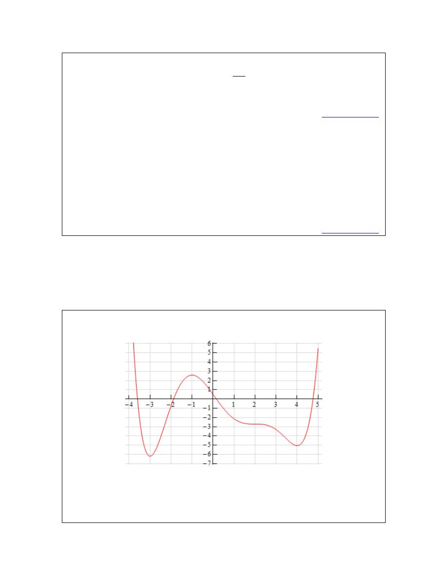
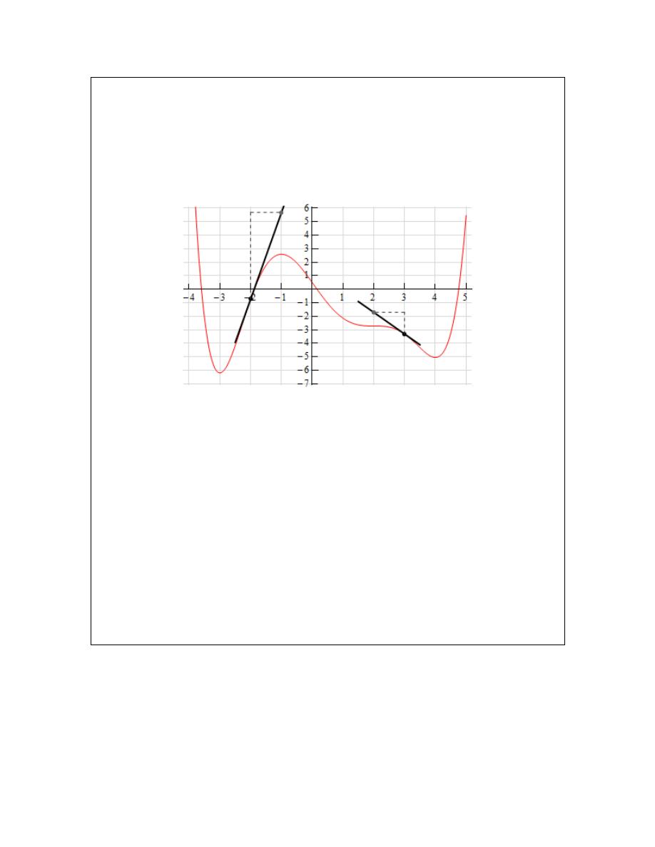
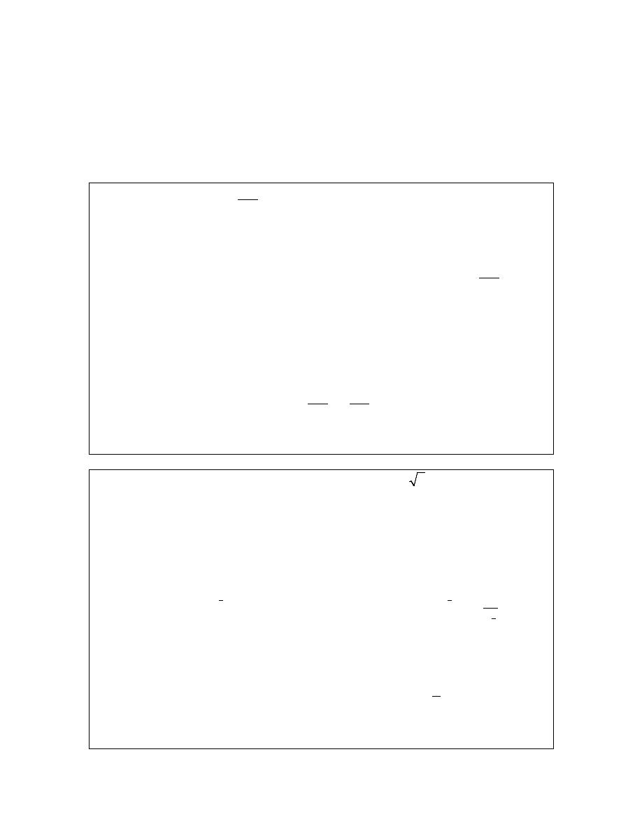
Example 4

Below is the sketch of a function

( )

f x

. Sketch the graph of the derivative of this

function,

( )

′

Solution
At first glance this seems to an all but impossible task. However, if you have some basic
knowledge of the interpretations of the derivative you can get a sketch of the derivative. It will
not be a perfect sketch for the most part, but you should be able to get most of the basic features

http://tutorial.math.lamar.edu/terms.aspx

Calculus I

of the derivative in the sketch.

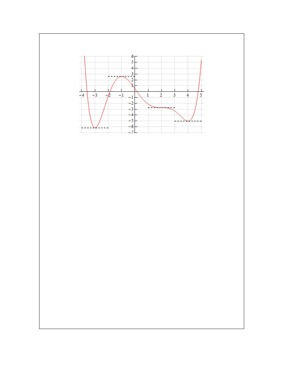
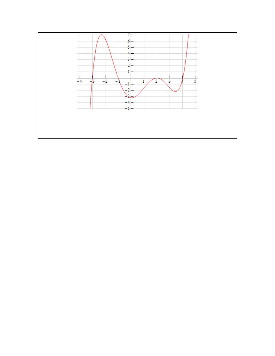
Let’s start off with the following sketch of the function with a couple of additions.

Notice that at

= −

and

the tangent line to the function is horizontal.

This means that the slope of the tangent line must be zero. Now, we know that the slope of the
tangent line at a particular point is also the value of the derivative of the function at that point.
Therefore, we now know that,

( )

′

− =

This is a good starting point for us. It gives us a few points on the graph of the derivative. It also
breaks the domain of the function up into regions where the function is increasing and decreasing.
We know, from our discussions above, that if the function is increasing at a point then the
derivative must be positive at that point. Likewise, we know that if the function is decreasing at a
point then the derivative must be negative at that point.

We can now give the following information about the derivative.

( )
( )
( )
( )
( )

′

< −

′

− < < −

′

− < <

′

< <

′

Remember that we are giving the signs of the derivatives here and these are solely a function of
whether the function is increasing or decreasing. The sign of the function itself is completely
immaterial here and will not in any way effect the sign of the derivative.

This may still seem like we don’t have enough information to get a sketch, but we can get a little

http://tutorial.math.lamar.edu/terms.aspx

Calculus I

bit more information about the derivative from the graph of the function. In the range

< −

know that the derivative must be negative, however we can also see that the derivative needs to

be increasing in this range. It is negative here until we reach

= −

and at this point the

derivative must be zero. The only way for the derivative to be negative to the left of

= −

and

zero at

= −

is for the derivative to increase as we increase x towards

= −

Now, in the range

− < < −

we know that the derivative must be zero at the endpoints and

positive in between the two endpoints. Directly to the right of

= −

the derivative must also be

increasing (because it starts at zero and then goes positive – therefore it must be increasing). So,
the derivative in this range must start out increasing and must eventually get back to zero at

= −

. So, at some point in this interval the derivative must start decreasing before it reaches

= −

. Now, we have to be careful here because this is just general behavior here at the two

endpoints. We won’t know where the derivative goes from increasing to decreasing and it may

well change between increasing and decreasing several times before we reach

= −

. All we

can really say is that immediately to the right of

= −

the derivative will be increasing and

immediately to the left of

= −

the derivative will be decreasing.

Next, for the ranges

− < <

and

< <

we know the derivative will be zero at the

endpoints and negative in between. Also, following the type of reasoning given above we can see
in each of these ranges that the derivative will be decreasing just to the right of the left hand
endpoint and increasing just to the left of the right hand endpoint.

Finally, in the last region

we know that the derivative is zero at

and positive to the

right of

. Once again, following the reasoning above, the derivative must also be increasing

in this range.

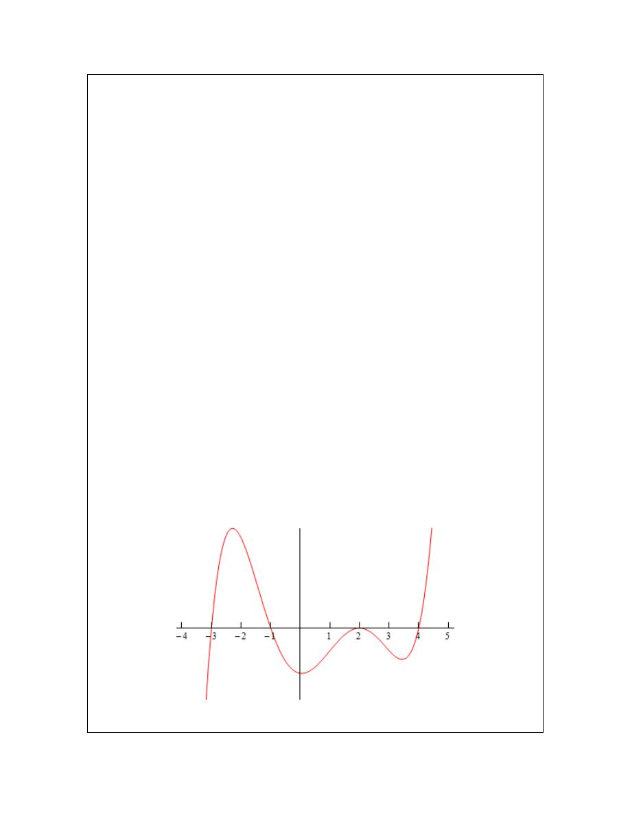
Putting all of this material together (and always taking the simplest choices for increasing and/or
decreasing information) gives us the following sketch for the derivative.

Note that this was done with the actual derivative and so is in fact accurate. Any sketch you do

http://tutorial.math.lamar.edu/terms.aspx

Calculus I

will probably not look quite the same. The “humps” in each of the regions may be at different
places and/or different heights for example. Also, note that we left off the vertical scale because
given the information that we’ve got at this point there was no real way to know this information.

That doesn’t mean however that we can’t get some ideas of specific points on the derivative other
than where we know the derivative to be zero. To see this let’s check out the following graph of
the function (not the derivative, but the function).

= −

and

we’ve sketched in a couple of tangent lines. We can use the basic rise/run

slope concept to estimate the value of the derivative at these points.

Let’s start at

. We’ve got two points on the line here. We can see that each seem to be

about one-quarter of the way off the grid line. So, taking that into account and the fact that we go
through one complete grid we can see that the slope of the tangent line, and hence the derivative,
is approximately -1.5.

= −

it looks like (with some heavy estimation) that the second point is about 6.5 grids

above the first point and so the slope of the tangent line here, and hence the derivative, is
approximately 6.5.

Here is the sketch of the derivative with the vertical scale included and from this we can see that
in fact our estimates are pretty close to reality.

http://tutorial.math.lamar.edu/terms.aspx

Calculus I

Note that this idea of estimating values of derivatives can be a tricky process and does require a
fair amount of (possible bad) approximations so while it can be used, you need to be careful with
it.

We’ll close out this section by noting that while we’re not going to include an example here we
could also use the graph of the derivative to give us a sketch of the function itself. In fact, in the
next chapter where we discuss some applications of the derivative we will be looking using
information the derivative gives us to sketch the graph of a function.

http://tutorial.math.lamar.edu/terms.aspx

Calculus I

Differentiation Formulas

In the first section of this chapter we saw the

definition of the derivative

and we computed a

couple of derivatives using the definition. As we saw in those examples there was a fair amount
of work involved in computing the limits and the functions that we worked with were not terribly
complicated.

For more complex functions using the definition of the derivative would be an almost impossible
task. Luckily for us we won’t have to use the definition terribly often. We will have to use it on
occasion, however we have a large collection of formulas and properties that we can use to
simplify our life considerably and will allow us to avoid using the definition whenever possible.

We will introduce most of these formulas over the course of the next several sections. We will
start in this section with some of the basic properties and formulas. We will give the properties
and formulas in this section in both “prime” notation and “fraction” notation.

Properties

( )

(

)

( )

f x

g x

′

( )

(

)

f x

g x

In other words, to differentiate a sum or difference all we need to do is differentiate the
individual terms and then put them back together with the appropriate signs. Note as well
that this property is not limited to two functions.

See the

Proof of Various Derivative Formulas

section of the Extras chapter to see the

proof of this property. It’s a very simple proof using the definition of the derivative.

( )

(

)

( )

cf x

′

( )

(

)

cf x

, c is any number

In other words, we can “factor” a multiplicative constant out of a derivative if we need to.
See the

Proof of Various Derivative Formulas

section of the Extras chapter to see the

proof of this property.

Note that we have not included formulas for the derivative of products or quotients of two
functions here. The derivative of a product or quotient of two functions is not the product or
quotient of the derivatives of the individual pieces. We will take a look at these in the next
section.

Next, let’s take a quick look at a couple of basic “computation” formulas that will allow us to
actually compute some derivatives.

http://tutorial.math.lamar.edu/terms.aspx

Calculus I

Formulas

1) If

( )

f x

then

( )

′

( )

The derivative of a constant is zero. See the

Proof of Various Derivative Formulas

section of the Extras chapter to see the proof of this formula.

2) If

( )

f x

then

( )

−

′

( )

−

, n is any number.

This formula is sometimes called the power rule. All we are doing here is bringing the
original exponent down in front and multiplying and then subtracting one from the
original exponent.

Note as well that in order to use this formula n must be a number, it can’t be a variable.
Also note that the base, the x, must be a variable, it can’t be a number. It will be tempting
in some later sections to misuse the Power Rule when we run in some functions where
the exponent isn’t a number and/or the base isn’t a variable.

See the

Proof of Various Derivative Formulas

section of the Extras chapter to see the

proof of this formula. There are actually three different proofs in this section. The first
two restrict the formula to n being an integer because at this point that is all that we can
do at this point. The third proof is for the general rule, but does suppose that you’ve read
most of this chapter.

These are the only properties and formulas that we’ll give in this section. Let’s compute some
derivatives using these properties.

Example 1

Differentiate each of the following functions.

(a)

( )

100

f x

−

[

Solution

]

(b)

( )

g t

−

[

Solution

]

(c)

−

+ −

[

Solution

]

(d)

( )

T x

−

[

Solution

]

(e)

( )

h x

−

[

Solution

]

Solution

(a)

( )

100

f x

−

In this case we have the sum and difference of four terms and so we will differentiate each of the
terms using the first property from above and then put them back together with the proper sign.
Also, for each term with a multiplicative constant remember that all we need to do is “factor” the
constant out (using the second property) and then do the derivative.

http://tutorial.math.lamar.edu/terms.aspx

Calculus I

( )

15 100

3 12

5 1

1500

′

−

Notice that in the third term the exponent was a one and so upon subtracting 1 from the original

exponent we get a new exponent of zero. Now recall that

. Don’t forget to do any basic

arithmetic that needs to be done such as any multiplication and/or division in the coefficients.

[

Return to Problems

]

(b)

( )

g t

−

The point of this problem is to make sure that you deal with negative exponents correctly. Here
is the derivative.

( ) ( )

( )

2 6

g t

−

′

+ −

−

Make sure that you correctly deal with the exponents in these cases, especially the negative
exponents. It is an easy mistake to “go the other way” when subtracting one off from a negative

exponent and get

−

instead of the correct

−

[

Return to Problems

]

(c)

−

+ −

Now in this function the second term is not correctly set up for us to use the power rule. The
power rule requires that the term be a variable to a power only and the term must be in the
numerator. So, prior to differentiating we first need to rewrite the second term into a form that
we can deal with.

−

+ −

Note that we left the 3 in the denominator and only moved the variable up to the numerator.
Remember that the only thing that gets an exponent is the term that is immediately to the left of
the exponent. If we’d wanted the three to come up as well we’d have written,

( )

so be careful with this! It’s a very common mistake to bring the 3 up into the numerator as well
at this stage.

Now that we’ve gotten the function rewritten into a proper form that allows us to use the Power
Rule we can differentiate the function. Here is the derivative for this part.

−

′ =

[

Return to Problems

]

http://tutorial.math.lamar.edu/terms.aspx

Calculus I

(d)

( )

T x

−

All of the terms in this function have roots in them. In order to use the power rule we need to
first convert all the roots to fractional exponents. Again, remember that the Power Rule requires
us to have a variable to a number and that it must be in the numerator of the term. Here is the
function written in “proper” form.

( )

T x

−

In the last two terms we combined the exponents. You should always do this with this kind of
term. In a later section we will learn of a technique that would allow us to differentiate this term
without combining exponents, however it will take significantly more work to do. Also don’t
forget to move the term in the denominator of the third term up to the numerator. We can now
differentiate the function.

( )

−

 





′

−

 





 





Make sure that you can deal with fractional exponents. You will see a lot of them in this class.

[

Return to Problems

]

(e)

( )

h x

−

In all of the previous examples the exponents have been nice integers or fractions. That is usually
what we’ll see in this class. However, the exponent only needs to be a number so don’t get
excited about problems like this one. They work exactly the same.

( )

2 1

h x

−

′

−

The answer is a little messy and we won’t reduce the exponents down to decimals. However, this
problem is not terribly difficult it just looks that way initially.

[

Return to Problems

]

There is a general rule about derivatives in this class that you will need to get into the habit of
using. When you see radicals you should always first convert the radical to a fractional exponent
and then simplify exponents as much as possible. Following this rule will save you a lot of grief
in the future.

http://tutorial.math.lamar.edu/terms.aspx

Calculus I

Back when we first put down the properties we noted that we hadn’t included a property for
products and quotients. That doesn’t mean that we can’t differentiate any product or quotient at
this point. There are some that we can do.

Example 2

Differentiate each of the following functions.

(a)

(

)

−

[

Solution

]

(b)

( )

h t

+ −

[

Solution

]

Solution

(a)

(

)

−

In this function we can’t just differentiate the first term, differentiate the second term and then
multiply the two back together. That just won’t work. We will discuss this in detail in the next
section so if you’re not sure you believe that hold on for a bit and we’ll be looking at that soon as
well as showing you an example of why it won’t work.

It is still possible to do this derivative however. All that we need to do is convert the radical to
fractional exponents (as we should anyway) and then multiply this through the parenthesis.

(

)

−

Now we can differentiate the function.

′ =

−

[

Return to Problems

]

(b)

( )

h t

+ −

As with the first part we can’t just differentiate the numerator and the denominator and the put it
back together as a fraction. Again, if you’re not sure you believe this hold on until the next
section and we’ll take a more detailed look at this.

We can simplify this rational expression however as follows.

( )

1 5

h t

−

+ −

This is a function that we can differentiate.

( )

h t

−

′

[

Return to Problems

]

http://tutorial.math.lamar.edu/terms.aspx

Calculus I

So, as we saw in this example there are a few products and quotients that we can differentiate. If
we can first do some simplification the functions will sometimes simplify into a form that can be
differentiated using the properties and formulas in this section.

Before moving on to the next section let’s work a couple of examples to remind us once again of
some of the interpretations of the derivative.

Example 3

( )

300

f x

increasing, decreasing or not changing at

= −

Solution
We know that the rate of change of a function is given by the functions derivative so all we need
to do is it rewrite the function (to deal with the second term) and then take the derivative.

( )

900

300

900

f x

−

′

⇒

−

Note that we rewrote the last term in the derivative back as a fraction. This is not something
we’ve done to this point and is only being done here to help with the evaluation in the next step.
It’s often easier to do the evaluation with positive exponents.

So, upon evaluating the derivative we get

( ) ( )

900

129

6 4

32.25

f ′

− =

−

= −

So, at

= −

the derivative is negative and so the function is decreasing at

= −

Example 4

Find the equation of the tangent line to

( )

f x

−

Solution
We know that the equation of a tangent line is given by,

( )

( )(

)

f a

x a

′

−

So, we will need the derivative of the function (don’t forget to get rid of the radical).

( )

4 4

f x

−

′

−

⇒

= −

Again, notice that we eliminated the negative exponent in the derivative solely for the sake of the
evaluation. All we need to do then is evaluate the function and the derivative at the point in

question,

( )

64 8 4

′

−

= − =

The tangent line is then,

(

)

32 3

−

http://tutorial.math.lamar.edu/terms.aspx

Calculus I

Example 5

The position of an object at any time t (in hours) is given by,

( )

s t

−

Determine when the object is moving to the right and when the object is moving to the left.

Solution
The only way that we’ll know for sure which direction the object is moving is to have the velocity
in hand. Recall that if the velocity is positive the object is moving off to the right and if the
velocity is negative then the object is moving to the left.

So, we need the derivative since the derivative is the velocity of the object. The derivative is,

( )

(

)

(

)(

)

s t

′

−

− +

−

The reason for factoring the derivative will be apparent shortly.

Now, we need to determine where the derivative is positive and where the derivative is negative.
There are several ways to do this. The method that I tend to prefer is the following.

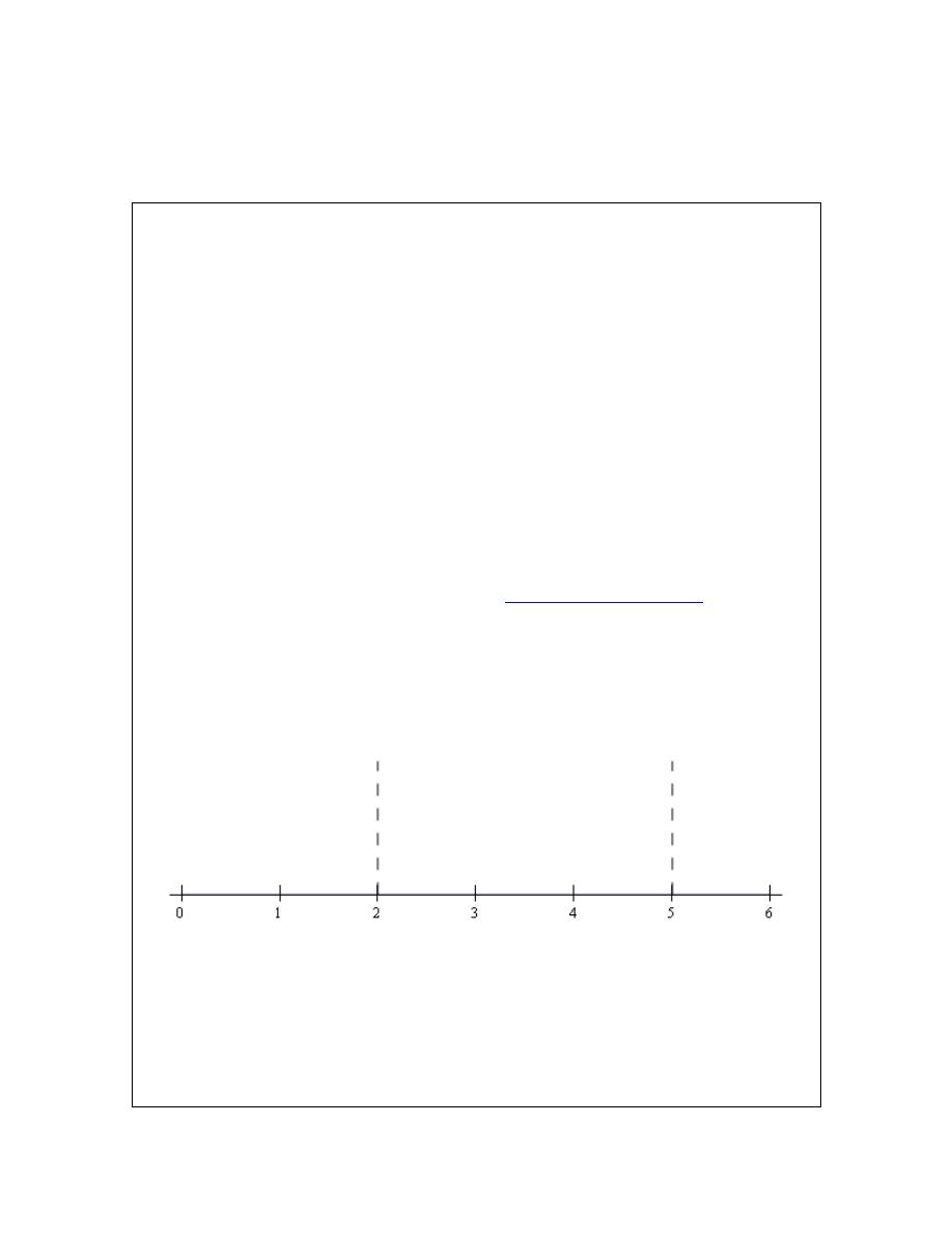
Since polynomials are continuous we know from the

Intermediate Value Theorem

that if the

polynomial ever changes sign then it must have first gone through zero. So, if we knew where
the derivative was zero we would know the only points where the derivative might change sign.

We can see from the factored form of the derivative that the derivative will be zero at

and

. Let’s graph these points on a number line.

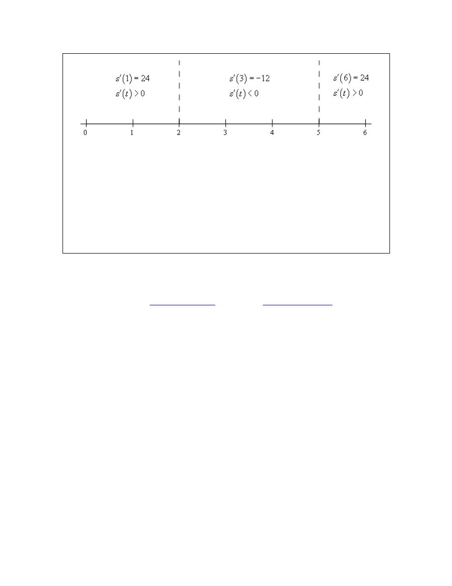
Now, we can see that these two points divide the number line into three distinct regions. In each
of these regions we know that the derivative will be the same sign. Recall the derivative can only
change sign at the two points that are used to divide the number line up into the regions.

Therefore, all that we need to do is to check the derivative at a test point in each region and the
derivative in that region will have the same sign as the test point. Here is the number line with
the test points and results shown.

http://tutorial.math.lamar.edu/terms.aspx

Calculus I

Here are the intervals in which the derivative is positive and negative.

positive :

2 & 5

negative :

−∞ < <

< < ∞

< <

We included negative t’s here because we could even though they may not make much sense for
this problem. Once we know this we also can answer the question. The object is moving to the
right and left in the following intervals.

moving to the right :

2 & 5

moving to the left :

−∞ < <

< < ∞

< <

Make sure that you can do the kind of work that we just did in this example. You will be asked
numerous times over the course of the next two chapters to determine where functions are
positive and/or negative. If you need some review or want to practice these kinds of problems
you should check out the

Solving Inequalities

section of my

Algebra/Trig Review

http://tutorial.math.lamar.edu/terms.aspx

Calculus I

Product and Quotient Rule

In the previous section we noted that we had to be careful when differentiating products or
quotients. It’s now time to look at products and quotients and see why.

First let’s take a look at why we have to be careful with products and quotients. Suppose that we

have the two functions

( )

f x

and

( )

g x

. Let’s start by computing the derivative of

the product of these two functions. This is easy enough to do directly.

( )

( ) ( )

f g

x x

′

′ =

Remember that on occasion we will drop the (x) part on the functions to simplify notation
somewhat. We’ve done that in the work above.

Now, let’s try the following.

( ) ( )

( )( )

x g x

′

So, we can very quickly see that.

( )

f g

′

′ ′

≠

In other words, the derivative of a product is not the product of the derivatives.

Using the same functions we can do the same thing for quotients.

( )

−

′





 





′

= −





 









 





( )

g x

′

So, again we can see that,

′

 

≠

 

′

 

To differentiate products and quotients we have the Product Rule and the Quotient Rule.

Product Rule
If the two functions f(x) and g(x) are differentiable (i.e. the derivative exist) then the product is
differentiable and,

( )

f g

′

The proof of the Product Rule is shown in the

Proof of Various Derivative Formulas

section of

the Extras chapter.

http://tutorial.math.lamar.edu/terms.aspx

Calculus I

Quotient Rule
If the two functions f(x) and g(x) are differentiable (i.e. the derivative exist) then the quotient is
differentiable and,

f g

′

 

−

 

 

Note that the numerator of the quotient rule is very similar to the product rule so be careful to not
mix the two up!

The proof of the Quotient Rule is shown in the

Proof of Various Derivative Formulas

section of

the Extras chapter.

Let’s do a couple of examples of the product rule.

Example 1

Differentiate each of the following functions.

(a)

(

)

−

[

Solution

]

(b)

( )

(

)

(

)

10 20

f x

−

[

Solution

]

Solution
At this point there really aren’t a lot of reasons to use the product rule. As we noted in the
previous section all we would need to do for either of these is to just multiply out the product and
then differentiate.

With that said we will use the product rule on these so we can see an example or two. As we add
more functions to our repertoire and as the functions become more complicated the product rule
will become more useful and in many cases required.

(a)

(

)

−

Note that we took the derivative of this function in the previous

section

and didn’t use the product

rule at that point. We should however get the same result here as we did then.

Now let’s do the problem here. There’s not really a lot to do here other than use the product rule.
However, before doing that we should convert the radical to a fractional exponent as always.

(

)

−

Now let’s take the derivative. So we take the derivative of the first function times the second
then add on to that the first function times the derivative of the second function.

(

)

(

)

2 2

−

′ =

−

http://tutorial.math.lamar.edu/terms.aspx

Calculus I

This is NOT what we got in the previous section for this derivative. However, with some
simplification we can arrive at the same answer.

′ =

−

This is what we got for an answer in the previous section so that is a good check of the product
rule.

[

Return to Problems

]

(b)

( )

(

)

(

)

10 20

f x

−

This one is actually easier than the previous one. Let’s just run it through the product rule.

( )

(

)

(

)

(

)

(

)

1 10 20

480

180

′

−

= −

−

Since it was easy to do we went ahead and simplified the results a little.

[

Return to Problems

]

Let’s now work an example or two with the quotient rule. In this case, unlike the product rule
examples, a couple of these functions will require the quotient rule in order to get the derivative.
The last two however, we can avoid the quotient rule if we’d like to as we’ll see.

Example 2

Differentiate each of the following functions.

(a)

( )

W z

−

[

Solution

]

(b)

( )

h x

−

[

Solution

]

(c)

( )

f x

[

Solution

]

(d)

[

Solution

]

Solution

(a)

( )

W z

−

There isn’t a lot to do here other than to use the quotient rule. Here is the work for this function.

( )

(

) (

)( )

(

)

(

)

3 2

− −

−

′

−

[

Return to Problems

]

http://tutorial.math.lamar.edu/terms.aspx

Calculus I

(b)

( )

h x

−

Again, not much to do here other than use the quotient rule. Don’t forget to convert the square
root into a fractional exponent.

( )

(

)

( )

(

)

(

)

(

)

h x

−

− −

′

−

[

Return to Problems

]

(c)

( )

f x

It seems strange to have this one here rather than being the first part of this example given that it
definitely appears to be easier than any of the previous two. In fact, it is easier. There is a point
to doing it here rather than first. In this case there are two ways to do compute this derivative.
There is an easy way and a hard way and in this case the hard way is the quotient rule. That’s the
point of this example.

Let’s do the quotient rule and see what we get.

( )

( ) ( )

( )

4 6

−

′

= −

Now, that was the “hard” way. So, what was so hard about it? Well actually it wasn’t that hard,
there is just an easier way to do it that’s all. However, having said that, a common mistake here
is to do the derivative of the numerator (a constant) incorrectly. For some reason many people
will give the derivative of the numerator in these kinds of problems as a 1 instead of 0! Also,
there is some simplification that needs to be done in these kinds of problems if you do the
quotient rule.

The easy way is to do what we did in the previous section.

( )

−

′

= −

Either way will work, but I’d rather take the easier route if I had the choice.

[

Return to Problems

]

http://tutorial.math.lamar.edu/terms.aspx

Calculus I

(d)

This problem also seems a little out of place. However, it is here again to make a point. Do not
confuse this with a quotient rule problem. While you can do the quotient rule on this function
there is no reason to use the quotient rule on this. Simply rewrite the function as

and differentiate as always.

′ =

[

Return to Problems

]

Finally, let’s not forget about our applications of derivatives.

Example 3

Suppose that the amount of air in a balloon at any time t is given by

( )

V t

Determine if the balloon is being filled with air or being drained of air at

Solution
If the balloon is being filled with air then the volume is increasing and if it’s being drained of air
then the volume will be decreasing. In other words, we need to get the derivative so that we can

determine the rate of change of the volume at

This will require the quotient rule.

( )

(

)

( )

(

)

(

)

(

)

V t

−

+ −

′

−

Note that we simplified the numerator more than usual here. This was only done to make the
derivative easier to evaluate.

The rate of change of the volume at

is then,

http://tutorial.math.lamar.edu/terms.aspx

Calculus I

( )

16 2

2178

242

−





′









= −

So, the rate of change of the volume at

is negative and so the volume must be decreasing.

Therefore air is being drained out of the balloon at

As a final topic let’s note that the product rule can be extended to more than two functions, for
instance.

(

)

(

)

f g h

f g h w

′

With this section and the previous section we are now able to differentiate powers of x as well as
sums, differences, products and quotients of these kinds of functions. However, there are many
more functions out there in the world that are not in this form. The next few sections give many
of these functions as well as give their derivatives.

http://tutorial.math.lamar.edu/terms.aspx

Calculus I

Derivatives of Trig Functions

With this section we’re going to start looking at the derivatives of functions other than
polynomials or roots of polynomials. We’ll start this process off by taking a look at the
derivatives of the six trig functions. Two of the derivatives will be derived. The remaining four
are left to the reader and will follow similar proofs for the two given here.

Before we actually get into the derivatives of the trig functions we need to give a couple of limits
that will show up in the derivation of two of the derivatives.

Fact

sin

cos

lim

→

−

See the

Proof of Trig Limits

section of the Extras chapter to see the proof of these two limits.

Before we start differentiating trig functions let’s work a quick set of limit problems that this fact
now allows us to do.

Example 1

Evaluate each of the following limits.

(a)

sin

lim

→

[

Solution

]

(b)

( )

sin 6

lim

→

[

Solution

]

(c)

( )

lim

sin 7

→

[

Solution

]

(d)

( )

sin 3

lim

sin 8

→

[

Solution

]

(e)

(

)

sin

lim

→

−

[

Solution

]

(f)

( )

cos 2

lim

→

−

[

Solution

]

Solution

(a)

sin

lim

→

There really isn’t a whole lot to this limit. In fact, it’s only here to contrast with the next example
so you can see the difference in how these work. In this case since there is only a 6 in the
denominator we’ll just factor this out and then use the fact.

( )

sin

lim

→

[

Return to Problems

]

http://tutorial.math.lamar.edu/terms.aspx

Calculus I

(b)

( )

sin 6

lim

→

Now, in this case we can’t factor the 6 out of the sine so we’re stuck with it there and we’ll need
to figure out a way to deal with it. To do this problem we need to notice that in the fact the

argument of the sine is the same as the denominator (i.e. both

’s). So we need to get both of the

argument of the sine and the denominator to be the same. We can do this by multiplying the
numerator and the denominator by 6 as follows.

( )

sin 6

6 sin 6

sin 6

lim

6 lim

→

Note that we factored the 6 in the numerator out of the limit. At this point, while it may not look
like it, we can use the fact above to finish the limit.

To see that we can use the fact on this limit let’s do a change of variables. A change of variables
is really just a renaming of portions of the problem to make something look more like something
we know how to deal with. They can’t always be done, but sometimes, such as this case, they

can simplify the problem. The change of variables here is to let

and then notice that as

→

we also have

( )

6 0

→

. When doing a change of variables in a limit we need to

change all the x’s into

’s and that includes the one in the limit.

Doing the change of variables on this limit gives,

( )

sin 6

lim

6 lim

let 6

sin

6 lim

6 1

→

=
=

And there we are. Note that we didn’t really need to do a change of variables here. All we really
need to notice is that the argument of the sine is the same as the denominator and then we can use
the fact. A change of variables, in this case, is really only needed to make it clear that the fact
does work.

[

Return to Problems

]

(c)

( )

lim

sin 7

→

In this case we appear to have a small problem in that the function we’re taking the limit of here
is upside down compared to that in the fact. This is not the problem it appears to be once we
notice that,

http://tutorial.math.lamar.edu/terms.aspx

Calculus I

( )

sin 7

and then all we need to do is recall a nice property of limits that allows us to do ,

( )

lim

sin 7

lim1

sin 7

lim

sin 7

lim

→

With a little rewriting we can see that we do in fact end up needing to do a limit like the one we
did in the previous part. So, let’s do the limit here and this time we won’t bother with a change of
variable to help us out. All we need to do is multiply the numerator and denominator of the
fraction in the denominator by 7 to get things set up to use the fact. Here is the work for this
limit.

( )

( )( )

lim

7 sin 7

sin 7

lim

sin 7

7 lim

7 1

→

[

Return to Problems

]

(d)

( )

sin 3

lim

sin 8

→

This limit looks nothing like the limit in the fact, however it can be thought of as a combination
of the previous two parts by doing a little rewriting. First, we’ll split the fraction up as follows,

( )

sin 3

lim

sin 8

→

Now, the fact wants a t in the denominator of the first and in the numerator of the second. This is

http://tutorial.math.lamar.edu/terms.aspx

Calculus I

easy enough to do if we multiply the whole thing by

(which is just one after all and so won’t

change the problem) and then do a little rearranging as follows,

( )

sin 3

lim

sin 8

sin 3

lim

sin 8

sin 3

lim

sin 8

t t

→

























At this point we can see that this really is two limits that we’ve seen before. Here is the work for
each of these and notice on the second limit that we’re going to work it a little differently than we
did in the previous part. This time we’re going to notice that it doesn’t really matter whether the
sine is in the numerator or the denominator as long as the argument of the sine is the same as
what’s in the numerator the limit is still one.

Here is the work for this limit.

( )

sin 3

3sin 3

lim

sin 8

8sin 8

sin 3

3lim

lim

sin 8

→

















































 

 

 

[

Return to Problems

]

(e)

(

)

sin

lim

→

−

This limit almost looks the same as that in the fact in the sense that the argument of the sine is the
same as what is in the denominator. However, notice that, in the limit, x is going to 4 and not 0 as
the fact requires. However, with a change of variables we can see that this limit is in fact set to
use the fact above regardless.

So, let

= − 4

and then notice that as

→

we have

→

. Therefore, after doing the

change of variable the limit becomes,

(

)

sin

lim

→

−

[

Return to Problems

]

http://tutorial.math.lamar.edu/terms.aspx

Calculus I

(f)

( )

cos 2

lim

→

−

The previous parts of this example all used the sine portion of the fact. However, we could just
have easily used the cosine portion so here is a quick example using the cosine portion to
illustrate this. We’ll not put in much explanation here as this really does work in the same
manner as the sine portion.

( )

(

)

( )

2 cos 2

cos 2

lim

cos 2

2 lim

2 0

→

−

All that is required to use the fact is that the argument of the cosine is the same as the
denominator.

[

Return to Problems

]

Okay, now that we’ve gotten this set of limit examples out of the way let’s get back to the main
point of this section, differentiating trig functions.

We’ll start with finding the derivative of the sine function. To do this we will need to use the
definition of the derivative. It’s been a while since we’ve had to use this, but sometimes there
just isn’t anything we can do about it. Here is the definition of the derivative for the sine
function.

( )

(

)

(

)

( )

sin

lim

→

−

Since we can’t just plug in

to evaluate the limit we will need to use the following trig

formula on the first sine in the numerator.

(

)

( ) ( )

sin

cos

sin

Doing this gives us,

( )

(

)

( ) ( )

( )

(

)

( ) ( )

( )

( ) ( )

sin

cos

sin

lim

sin

cos

sin

lim

cos

sin

lim sin

lim cos

→

−

− +

−

http://tutorial.math.lamar.edu/terms.aspx

Calculus I

As you can see upon using the trig formula we can combine the first and third term and then
factor a sine out of that.  We can then break up the fraction into two pieces, both of which can be
dealt with separately.

Now, both of the limits here are limits as h approaches zero. In the first limit we have a sin(x)
and in the second limit we have a cos(x). Both of these are only functions of x only and as h
moves in towards zero this has no affect on the value of x.  Therefore, as far as the limits are
concerned, these two functions are constants and can be factored out of their respective limits.
Doing this gives,

( )

(

)

( )

cos

sin

lim

cos

lim

→

−

At this point all we need to do is use the limits in the fact above to finish out this problem.

( )

(

)

( )( )

( )

sin

cos

Differentiating cosine is done in a similar fashion. It will require a different trig formula, but
other than that is an almost identical proof. The details will be left to you. When done with the
proof you should get,

( )

(

)

( )

cos

sin

= −

With these two out of the way the remaining four are fairly simple to get. All the remaining four
trig functions can be defined in terms of sine and cosine and these definitions, along with
appropriate derivative rules, can be used to get their derivatives.

Let’s take a look at tangent. Tangent is defined as,

( )

sin

tan

cos

Now that we have the derivatives of sine and cosine all that we need to do is use the quotient rule
on this. Let’s do that.

( )

(

)

( )

( ) ( )

( )

(

)

( )

(

)

( )

sin

tan

cos

sin

cos

sin

cos

















−

http://tutorial.math.lamar.edu/terms.aspx

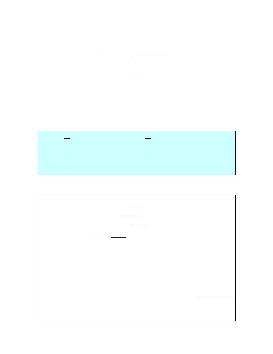
Calculus I

Now, recall that

( )

cos

sin

and if we also recall the definition of secant in terms of

cosine we arrive at,

( )

(

)

( )

cos

sin

tan

cos

sec

The remaining three trig functions are also quotients involving sine and/or cosine and so can be
differentiated in a similar manner. We’ll leave the details to you. Here are the derivatives of all
six of the trig functions.

Derivatives of the six trig functions

( )

(

)

( )

(

)

( )

(

)

( )

(

)

( )

(

)

( ) ( )

( )

(

)

( ) ( )

sin

cos

sin

tan

sec

cot

csc

sec

tan

csc

cot

= −

At this point we should work some examples.

Example 2

Differentiate each of the following functions.

(a)

( )

3sec

10 cot

g x

−

[

Solution

]

(b)

( )

tan

h w

−

[

Solution

]

(c)

( ) ( )

( )

5sin

cos

4 csc

[

Solution

]

(d)

( )

sin

3 2 cos

P t

−

[

Solution

]

Solution

(a)

( )

3sec

10 cot

g x

−

There really isn’t a whole lot to this problem. We’ll just differentiate each term using the
formulas from above.

( )

( ) ( )

( )

(

)

( ) ( )

( )

3sec

tan

csc

3sec

tan

10 csc

g x

′

−

[

Return to Problems

]

(b)

( )

tan

h w

−

In this part we will need to use the product rule on the second term and note that we really will
need the product rule here. There is no other way to do this derivative unlike what we saw when

http://tutorial.math.lamar.edu/terms.aspx

Calculus I

we first looked at the product rule. When we first looked at the product rule the only functions
we knew how to differentiate were polynomials and in those cases all we really needed to do was
multiply them out and we could take the derivative without the product rule. We are now getting
into the point where we will be forced to do the product rule at times regardless of whether or not
we want to.

We will also need to be careful with the minus sign in front of the second term and make sure that
it gets dealt with properly. There are two ways to deal with this. One way it to make sure that
you use a set of parenthesis as follows,

( )

(

)

( )

2 tan

sec

2 tan

sec

h w

−

′

= −

−

= −

−

Because the second term is being subtracted off of the first term then the whole derivative of the
second term must also be subtracted off of the derivative of the first term. The parenthesis make
this idea clear.

A potentially easier way to do this is to think of the minus sign as part of the first function in the

product. Or, in other words the two functions in the product, using this idea, are

−

and

( )

tan w

. Doing this gives,

( )

2 tan

sec

h w

−

′

= −

−

So, regardless of how you approach this problem you will get the same derivative.

[

Return to Problems

]

(c)

( ) ( )

( )

5sin

cos

4 csc

As with the previous part we’ll need to use the product rule on the first term. We will also think
of the 5 as part of the first function in the product to make sure we deal with it correctly.
Alternatively, you could make use of a set of parenthesis to make sure the 5 gets dealt with
properly. Either way will work, but we’ll stick with thinking of the 5 as part of the first term in
the product. Here’s the derivative of this function.

( ) ( )

( )

(

)

( ) ( )

( )

( ) ( )

5 cos

cos

5sin

sin

4 csc

cot

5 cos

5sin

4 csc

cot

′ =

−

[

Return to Problems

]

(d)

( )

sin

3 2 cos

P t

−

In this part we’ll need to use the quotient rule to take the derivative.

http://tutorial.math.lamar.edu/terms.aspx

Calculus I

( )

(

)

( )

(

)

( )

(

)

( )

(

)

cos

3 2 cos

sin

2 sin

3 2 cos

3cos

2 cos

2 sin

3 2 cos

P t

−

′

−

Be careful with the signs when differentiating the denominator. The negative sign we get from
differentiating the cosine will cancel against the negative sign that is already there.

This appears to be done, but there is actually a fair amount of simplification that can yet be done.
To do this we need to factor out a “-2” from the last two terms in the numerator and the make use

of the fact that

( )

cos

sin

( )

(

)

( )

(

)

( )

(

)

3cos

2 cos

sin

3 2 cos

3cos

3 2 cos

P t

−

′

−

[

Return to Problems

]

As a final problem here let’s not forget that we still have our standard interpretations to
derivatives.

Example 3

Suppose that the amount of money in a bank account is given by

( )

500 100 cos

150 sin

P t

−

where t is in years. During the first 10 years in which the account is open when is the amount of
money in the account increasing?

Solution
To determine when the amount of money is increasing we need to determine when the rate of
change is positive. Since we know that the rate of change is given by the derivative that is the
first thing that we need to find.

( )

100 sin

150 cos

P t

′

= −

−

Now, we need to determine where in the first 10 years this will be positive. This is equivalent to
asking where in the interval [0, 10] is the derivative positive. Recall that both sine and cosine are
continuous functions and so the derivative is also a continuous function. The

Intermediate Value

Theorem

then tells us that the derivative can only change sign if it first goes through zero.

So, we need to solve the following equation.

http://tutorial.math.lamar.edu/terms.aspx

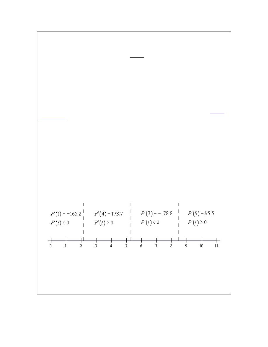
Calculus I

( )

( )
( )

( )

100 sin

150 cos

100 sin

150 cos

sin

1.5

cos

tan

1.5

−

=
= −

= −

The solution to this equation is,

2.1588 2

0, 1, 2,

5.3004 2

0, 1, 2,

π
π

= ± ±




If you don’t recall how to solve trig equations go back and take a look at the sections on

solving

trig equations

in the Review chapter.

We are only interested in those solutions that fall in the range [0, 10]. Plugging in values of n
into the solutions above we see that the values we need are,

2.1588

2.1588 2

8.4420

5.3004

So, much like solving polynomial inequalities all that we need to do is sketch in a number line
and add in these points. These points will divide the number line into regions in which the
derivative must always be the same sign. All that we need to do then is choose a test point from
each region to determine the sign of the derivative in that region.

Here is the number line with all the information on it.

So, it looks like the amount of money in the bank account will be increasing during the following
intervals.

2.1588

5.3004

8.4420

< <

Note that we can’t say anything about what is happening after

since we haven’t done any

work for t’s after that point.

In this section we saw how to differentiate trig functions. We also saw in the last example that
our interpretations of the derivative are still valid so we can’t forget those.

http://tutorial.math.lamar.edu/terms.aspx

Calculus I

Also, it is important that we be able to solve trig equations as this is something that will arise off
and on in this course. It is also important that we can do the kinds of number lines that we used
in the last example to determine where a function is positive and where a function is negative.
This is something that we will be doing on occasion in both this chapter and the next.

http://tutorial.math.lamar.edu/terms.aspx

Calculus I

Derivatives of Exponential and Logarithm Functions

The next set of functions that we want to take a look at are exponential and logarithm functions.
The most common exponential and logarithm functions in a calculus course are the natural

exponential function,

, and the natural logarithm function,

( )

ln x

. We will take a more

general approach however and look at the general exponential and logarithm function.

Exponential Functions
We’ll start off by looking at the exponential function,

( )

f x

We want to differentiate this. The power rule that we looked at a couple of sections ago won’t
work as that required the exponent to be a fixed number and the base to be a variable. That is
exactly the opposite from what we’ve got with this function. So, we’re going to have to start with
the definition of the derivative.

( )

(

)

( )

(

)

lim

x h

f x

a a

→

−

′

−

Now, the

is not affected by the limit since it doesn’t have any h’s in it and so is a constant as

far as the limit is concerned. We can therefore factor this out of the limit. This gives,

( )

lim

→

−

′

Now let’s notice that the limit we’ve got above is exactly the definition of the derivative of

( )

f x

, i.e.

( )

f ′

. Therefore, the derivative becomes,

( )

′

So, we are kind of stuck. We need to know the derivative in order to get the derivative!

There is one value of a that we can deal with at this point. Back in the

Exponential Functions

section of the Review chapter we stated that

2.71828182845905



What we didn’t do

however is actually define where e comes from. There are in fact a variety of ways to define e.
Here are three of them.

http://tutorial.math.lamar.edu/terms.aspx

Calculus I

Some Definitions of e.

lim 1

→∞













2. e is the unique positive number for which

lim

→

−

∞

∑

The second one is the important one for us because that limit is exactly the limit that we’re
working with above. So, this definition leads to the following fact,

Fact 1

For the natural exponential function,

( )

f x

= e

we have

( )

lim

→

−

′

So, provided we are using the natural exponential function we get the following.

( )

f x

′

⇒

At this point we’re missing some knowledge that will allow us to easily get the derivative for a
general function.

Eventually

we will be able to show that for a general exponential function we

have,

( )

f x

′

⇒

Logarithm Functions
Let’s now briefly get the derivatives for logarithms. In this case we will need to start with the
following fact about functions that are inverses of each other.

Fact 2
If f(x) and g(x) are inverses of each other then,

( )

(

)

g x

′

So, how is this fact useful to us? Well

recall

that the natural exponential function and the natural

logarithm function are inverses of each other and we know what the derivative of the natural
exponential function is!

So, if we have

( )

f x

= e

and

( )

g x

then,

http://tutorial.math.lamar.edu/terms.aspx

Calculus I

( )

(

)

( )

g x

′

The last step just uses the fact that the two functions are inverses of each other.

Putting this all together gives,

( )

Note that we need to require that

since this is required for the logarithm and so must also

be required for its derivative. It can also be shown that,

(

)

≠

Using this all we need to avoid is

In this case, unlike the exponential function case, we can actually find the derivative of the
general logarithm function. All that we need is the derivative of the natural logarithm, which we
just found, and the

change of base formula

. Using the change of base formula we can write a

general logarithm as,

log

Differentiation is then fairly simple.

(

)

( )

log

a dx













We took advantage of the fact that a was a constant and so

ln a

is also a constant and can be

factored out of the derivative. Putting all this together gives,

(

)

log

Here is a summary of the derivatives in this section.

( )

(

)

log

http://tutorial.math.lamar.edu/terms.aspx

Calculus I

Okay, now that we have the derivations of the formulas out of the way let’s compute a couple of
derivatives.

Example 1

Differentiate each of the following functions.

(a)

( )

5 log

R w

−

(b)

( )

f x

(c)

Solution
(a) This will be the only example that doesn’t involve the natural exponential and natural
logarithm functions.

( )

4 ln 4

ln 9

R w

′

−

(b) Not much to this one. Just remember to use the product rule on the second term.

( )

 

′

 

 

(c) We’ll need to use the quotient rule on this one.

(

) ( )( )

(

)

(

)

(

)

+ −

′ =

−

There’s really not a lot to differentiating natural logarithms and natural exponential functions at
this point as long as you remember the formulas. In later sections as we get more formulas under
our belt they will become more complicated.

Next, we need to do our obligatory application/interpretation problem so we don’t forget about
them.

Example 2

Suppose that the position of an object is given by

( )

s t

= e

Does the object ever stop moving?

Solution
First we will need the derivative. We need this to determine if the object ever stops moving since

http://tutorial.math.lamar.edu/terms.aspx

Calculus I

at that point (provided there is one) the velocity will be zero and recall that the derivative of the
position function is the velocity of the object.

The derivative is,

( )

(

)

s t

′

= +

So, we need to determine if the derivative is ever zero. To do this we will need to solve,

(

)

Now, we know that exponential functions are never zero and so this will only be zero at

= −

So, if we are going to allow negative values of t then the object will stop moving once at

= −

If we aren’t going to allow negative values of t then the object will never stop moving.

Before moving on to the next section we need to go back over a couple of derivatives to make
sure that we don’t confuse the two. The two derivatives are,

( )
( )

Power Rule

Derivative of an exponential function

−

It is important to note that with the Power rule the exponent MUST be a constant and the base
MUST be a variable while we need exactly the opposite for the derivative of an exponential
function. For an exponential function the exponent MUST be a variable and the base MUST be a
constant.

It is easy to get locked into one of these formulas and just use it for both of these. We also
haven’t even talked about what to do if both the exponent and the base involve variables. We’ll
see this situation in a later

section

http://tutorial.math.lamar.edu/terms.aspx

Calculus I

Derivatives of Inverse Trig Functions

In this section we are going to look at the derivatives of the inverse trig functions. In order to
derive the derivatives of inverse trig functions we’ll need the formula from the last section
relating the derivatives of inverse functions. If f(x) and g(x) are inverse functions then,

( )

(

)

g x

′

Recall as well that two functions are inverses if

( )

(

)

f g x

and

( )

(

)

g f x

We’ll go through inverse sine, inverse cosine and inverse tangent in detail here and leave the
other three to you to derive if you’d like to.

Inverse Sine
Let’s start with inverse sine. Here is the definition of the inverse sine.

sin

for

−

⇔

− ≤ ≤

So, evaluating an inverse trig function is the same as asking what angle (i.e. y) did we plug into
the sine function to get x. The restrictions on y given above are there to make sure that we get a
consistent answer out of the inverse sine. We know that there are in fact an infinite number of
angles that will work and we want a consistent value when we work with inverse sine. Using the
range of angles above gives all possible values of the sine function exactly once. If you’re not
sure of that sketch out a unit circle and you’ll see that that range of angles (the y’s) will cover all
possible values of sine.

Note as well that since

( )

1 sin

− ≤

≤

we also have

− ≤ ≤

Let’s work a quick example.

Example 1

Evaluate

sin

−

 

 

 

Solution
So we are really asking what angle y solves the following equation.

( )

sin

and we are restricted to the values of y above.

From a unit circle we can quickly see that

We have the following relationship between the inverse sine function and the sine function.

http://tutorial.math.lamar.edu/terms.aspx

Calculus I

(

)

(

)

sin sin

sin

−

In other words they are inverses of each other. This means that we can use the fact above to find
the derivative of inverse sine. Let’s start with,

( )

sin

f x

g x

−

Then,

( )

(

)

(

)

cos sin

g x

−

′

This is not a very useful formula. Let’s see if we can get a better formula. Let’s start by recalling
the definition of the inverse sine function.

( )

sin

−

⇒

Using the first part of this definition the denominator in the derivative becomes,

(

)

( )

cos sin

cos

−

Now, recall that

cos

sin

cos

1 sin

⇒

−

Using this, the denominator is now,

(

)

( )

cos sin

cos

1 sin

−

Now, use the second part of the definition of the inverse sine function. The denominator is then,

(

)

cos sin

1 sin

−

Putting all of this together gives the following derivative.

(

)

sin

−

Inverse Cosine
Now let’s take a look at the inverse cosine. Here is the definition for the inverse cosine.

cos

for

−

⇔

≤ ≤

As with the inverse since we’ve got a restriction on the angles, y, that we get out of the inverse
cosine function. Again, if you’d like to verify this a quick sketch of a unit circle should convince
you that this range will cover all possible values of cosine exactly once. Also, we also have

− ≤ ≤

because

( )

1 cos

− ≤

≤

http://tutorial.math.lamar.edu/terms.aspx

Calculus I

Example 2

Evaluate

cos

−





−













Solution
As with the inverse sine we are really just asking the following.

cos

= −

where y must meet the requirements given above. From a unit circle we can see that we must

have

The inverse cosine and cosine functions are also inverses of each other and so we have,

(

)

(

)

cos cos

cos

−

To find the derivative we’ll do the same kind of work that we did with the inverse sine above. If
we start with

( )

cos

f x

g x

−

then,

( )

(

)

(

)

sin cos

g x

−

′

−

Simplifying the denominator here is almost identical to the work we did for the inverse sine and
so isn’t shown here. Upon simplifying we get the following derivative.

(

)

cos

−

= −

−

So, the derivative of the inverse cosine is nearly identical to the derivative of the inverse sine.
The only difference is the negative sign.

Inverse Tangent
Here is the definition of the inverse tangent.

tan

for

−

⇔

− < <

Again, we have a restriction on y, but notice that we can’t let y be either of the two endpoints in
the restriction above since tangent isn’t even defined at those two points. To convince yourself
that this range will cover all possible values of tangent do a quick

sketch

of the tangent function

and we can see that in this range we do indeed cover all possible values of tangent. Also, in this
case there are no restrictions on x because tangent can take on all possible values.

http://tutorial.math.lamar.edu/terms.aspx

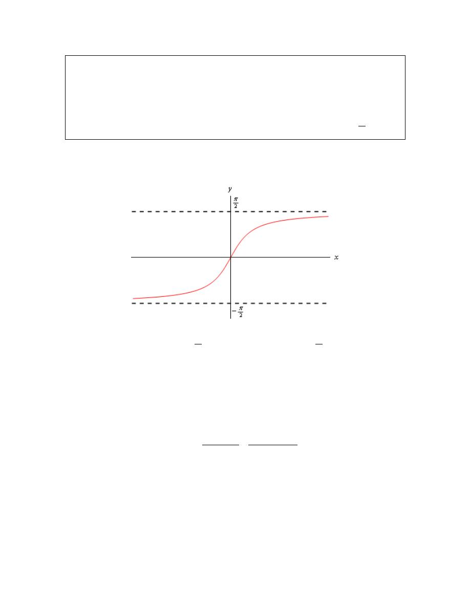
Calculus I

Example 3

Evaluate

tan 1

−

Solution
Here we are asking,

tan

where y satisfies the restrictions given above. From a unit circle we can see that

Because there is no restriction on x we can ask for the limits of the inverse tangent function as x
goes to plus or minus infinity. To do this we’ll need the graph of the inverse tangent function.
This is shown below.

From this graph we can see that

lim tan

−

→∞

→−∞

= −

The tangent and inverse tangent functions are inverse functions so,

(

)

(

)

tan tan

tan

−

Therefore to find the derivative of the inverse tangent function we can start with

( )

tan

f x

g x

−

We then have,

( )

(

)

(

)

sec

tan

g x

−

′

Simplifying the denominator is similar to the inverse sine, but different enough to warrant
showing the details. We’ll start with the definition of the inverse tangent.

tan

−

⇒

The denominator is then,

(

)

sec

tan

sec

−

http://tutorial.math.lamar.edu/terms.aspx

Calculus I

Now, if we start with the fact that

cos

sin

and divide every term by cos

y we will get,

1 tan

sec

The denominator is then,

(

)

sec

tan

sec

1 tan

−

= +

Finally using the second portion of the definition of the inverse tangent function gives us,

(

)

sec

tan

1 tan

−

= +

The derivative of the inverse tangent is then,

(

)

tan

−

There are three more inverse trig functions but the three shown here the most common ones.
Formulas for the remaining three could be derived by a similar process as we did those above.
Here are the derivatives of all six inverse trig functions.

(

)

(

)

(

)

(

)

(

)

(

)

sin

cos

tan

cot

sec

csc

−

= −

−

= −

−

We should probably now do a couple of quick derivatives here before moving on to the next
section.

Example 4

Differentiate the following functions.

(a)

( )

4 cos

10 tan

f t

−

(b)

( )

sin

−

Solution
(a) Not much to do with this one other than differentiate each term.

( )

′

= −

−

http://tutorial.math.lamar.edu/terms.aspx

Calculus I

(b) Don’t forget to convert the radical to fractional exponents before using the product rule.

( )

sin

−

′ =

−

Alternate Notation
There is some alternate notation that is used on occasion to denote the inverse trig functions. This
notation is,

sin

arcsin

cos

arccos

tan

arctan

cot

arccot

sec

arcsec

csc

arccsc

−

http://tutorial.math.lamar.edu/terms.aspx

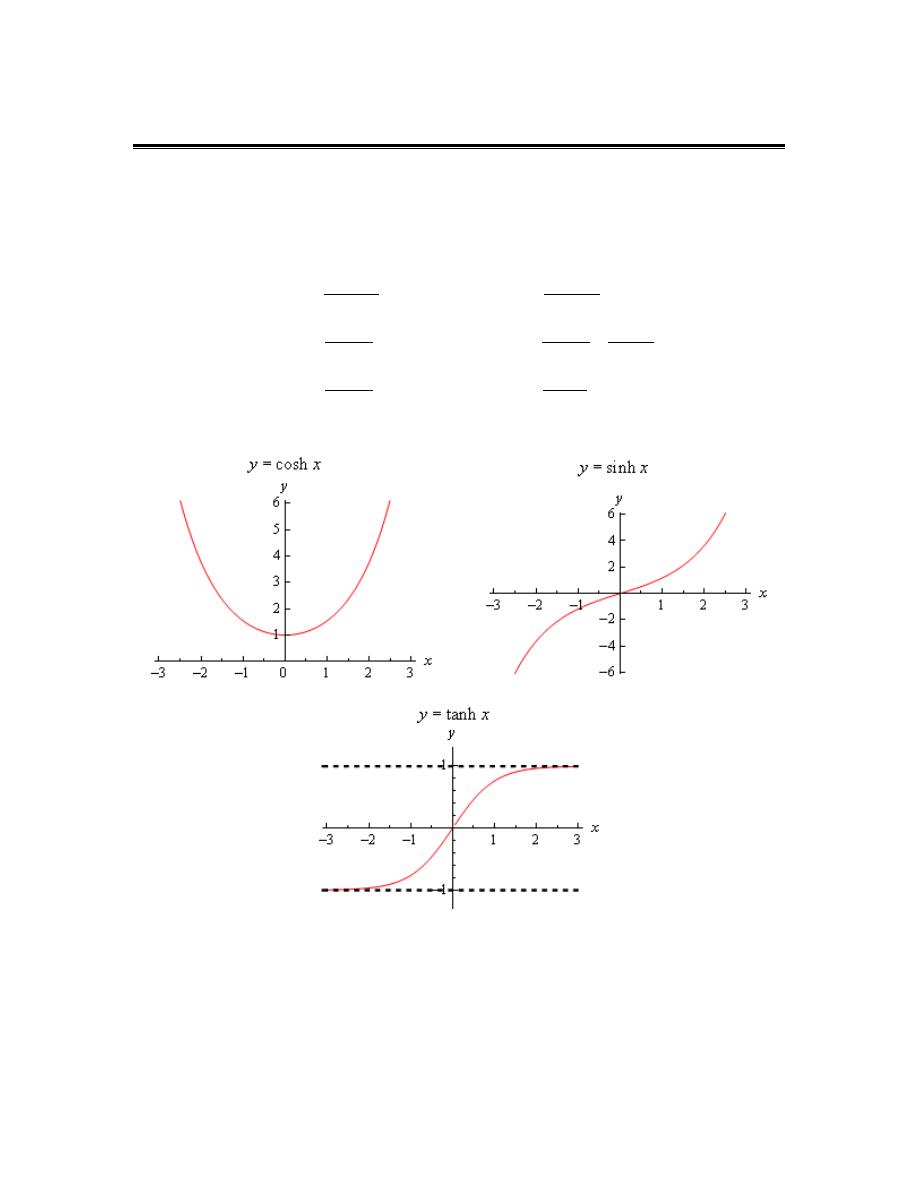
Calculus I

Derivatives of Hyperbolic Functions

The last set of functions that we’re going to be looking in this chapter at are the hyperbolic

functions. In many physical situations combinations of

and

−

arise fairly often. Because of

this these combinations are given names. There are six hyperbolic functions and they are defined
as follows.

sinh

cosh

sinh

cosh

tanh

coth

cosh

sinh

tanh

sech

csch

cosh

sinh

−

Here are the graphs of the three main hyperbolic functions.

We also have the following facts about the hyperbolic functions.

( )

sinh

cosh

sinh

1 tanh

sech

− = −

− =

−

You’ll note that these are similar, but not quite the same, to some of the more common trig
identities so be careful to not confuse the identities here with those of the standard trig functions.

http://tutorial.math.lamar.edu/terms.aspx

Calculus I

Because the hyperbolic functions are defined in terms of exponential functions finding their
derivatives is fairly simple provided you’ve already read through the next section. We haven’t
however so we’ll need the following formula that can be easily proved after we’ve covered the
next section.

( )

−

= −

With this formula we’ll do the derivative for hyperbolic sine and leave the rest to you as an
exercise.

(

)

(

)

sinh

cosh

−

− −





−









For the rest we can either use the definition of the hyperbolic function and/or the quotient rule.
Here are all six derivatives.

(

)

(

)

(

)

(

)

(

)

(

)

sinh

cosh

sinh

tanh

sech

coth

csch

sech

sech tanh

csch

csch coth

= −

Here are a couple of quick derivatives using hyperbolic functions.

Example 1

Differentiate each of the following functions.

(a)

( )

cosh

f x

(b)

( )

sinh

h t

Solution
(a)

( )

cosh

sinh

′

(b)

( ) (

)

(

)

1 cosh

sinh

h t

−

′

http://tutorial.math.lamar.edu/terms.aspx

Calculus I

Chain Rule

We’ve taken a lot of derivatives over the course of the last few sections. However, if you look
back they have all been functions similar to the following kinds of functions.

( )

tan

R z

f t

h w

g x

These are all fairly simple functions in that wherever the variable appears it is by itself. What
about functions like the following,

( )

(

)

( )

(

)

( )

(

)

cos

tan

tan 5

R z

f t

h w

g x

−

None of our rules will work on these functions and yet some of these functions are closer to the
derivatives that we’re liable to run into than the functions in the first set.

Let’s take the first one for example. Back in the

section

on the definition of the derivative we

actually used the definition to compute this derivative. In that section we found that,

( )

2 5

R z

′

−

If we were to just use the power rule on this we would get,

(

)

2 5

−

which is not the derivative that we computed using the definition. It is close, but it’s not the
same. So, the power rule alone simply won’t work to get the derivative here.

Let’s keep looking at this function and note that if we define,

( )

f z

g z

−

then we can write the function as a composition.

( ) (

)( )

( )

(

)

R z

f g z

−



and it turns out that it’s actually fairly simple to differentiate a function composition using the
Chain Rule. There are two forms of the chain rule. Here they are.

Chain Rule
Suppose that we have two functions f(x) and g(x) and they are both differentiable.

1. If we define

( ) (

)( )

F x



then the derivative of F(x) is,

( )

(

)

( )

F x

g x

′

2. If we have

( )

f u

and

( )

g x

then the derivative of y is,

dy du

du dx

http://tutorial.math.lamar.edu/terms.aspx

Calculus I

Each of these forms have their uses, however we will work mostly with the first form in this
class. To see the proof of the Chain Rule see the

Proof of Various Derivative Formulas

section of

the Extras chapter.

Now, let’s go back and use the Chain Rule on the function that we used when we opened this
section.

Example 1

Use the Chain Rule to differentiate

( )

R z

−

Solution
We’ve already identified the two functions that we needed for the composition, but let’s write
them back down anyway and take their derivatives.

( )

f z

g z

−

′

So, using the chain rule we get,

( )

(

)

( )

(

) ( )

(

) ( )

( )

2 5

R z

g z

−

′

−

And this is what we got using the definition of the derivative.

In general we don’t really do all the composition stuff in using the Chain Rule. That can get a
little complicated and in fact obscures the fact that there is a quick and easy way of remembering
the chain rule that doesn’t require us to think in terms of function composition.

Let’s take the function from the previous example and rewrite it slightly.

( ) (

)



outside

inside function function

R z

−







This function has an “inside function” and an “outside function”. The outside function is the

square root or the exponent of

1
2

depending on how you want to think of it and the inside

http://tutorial.math.lamar.edu/terms.aspx

Calculus I

function is the stuff that we’re taking the square root of or raising to the

1
2

, again depending on

how you want to look at it.

The derivative is then,

( )

(

)

( )

derivative of

outside function

inside function

derivative of

left alone

inside function

R z

−

′

−















In general this is how we think of the chain rule. We identify the “inside function” and the
“outside function”. We then differentiate the outside function leaving the inside function alone
and multiply all of this by the derivative of the inside function. In its general form this is,

( )

(

)

( )

derivative of

times derivative

inside function

outside function

of inside function

left alone

F x

g x

′

= 









We can always identify the “outside function” in the examples below by asking ourselves how we
would evaluate the function. For instance in the R(z) case if we were to ask ourselves what R(2)
is we would first evaluate the stuff under the radical and then finally take the square root of this
result. The square root is the last operation that we perform in the evaluation and this is also the
outside function. The outside function will always be the last operation you would perform if you
were going to evaluate the function.

Let’s take a look at some examples of the Chain Rule.

Example 2

Differentiate each of the following.

(a)

( )

(

)

sin 3

f x

[

Solution

]

(b)

( )

(

)

cos

f t

[

Solution

]

(c)

( )

h w

−

= e

[

Solution

]

(d)

( )

(

)

g x

−

[

Solution

]

(e)

(

)

sec 1 5

−

[

Solution

]

(f)

( )

cos

P t

[

Solution

]

Solution

(a)

( )

(

)

sin 3

f x

It looks like the outside function is the sine and the inside function is 3x

+x. The derivative is

then.

( )

(

)

(

)

derivative of

times derivative

leave inside

outside function

of inside function

function alone

cos

′











http://tutorial.math.lamar.edu/terms.aspx

Calculus I

Or with a little rewriting,

( ) (

)

(

)

1 cos 3

′

[

Return to Problems

]

(b)

( )

(

)

cos

f t

In this case the outside function is the exponent of 50 and the inside function is all the stuff on the
inside of the parenthesis. The derivative is then.

( )

(

)

( )

(

)

( )

(

)

( )

(

)

50 2

cos

sin

50 6

sin

cos

′

−

[

Return to Problems

]

(c)

( )

h w

−

= e

Identifying the outside function in the previous two was fairly simple since it really was the
“outside” function in some sense. In this case we need to be a little careful. Recall that the
outside function is the last operation that we would perform in an evaluation. In this case if we
were to evaluate this function the last operation would be the exponential. Therefore the outside
function is the exponential function and the inside function is its exponent.

Here’s the derivative.

( )

(

)

(

)

h w

−

′

−

Remember, we leave the inside function alone when we differentiate the outside function. So, the
derivative of the exponential function (with the inside left alone) is just the original function.

[

Return to Problems

]

(d)

( )

(

)

g x

−

Here the outside function is the natural logarithm and the inside function is stuff on the inside of
the logarithm.

( )

(

)

g x

−

′

−

Again remember to leave the inside function along when differentiating the outside function. So,
upon differentiating the logarithm we end up not with 1/x but instead with 1/(inside function).

[

Return to Problems

]

(e)

(

)

sec 1 5

−

In this case the outside function is the secant and the inside is the

1 5x

−

http://tutorial.math.lamar.edu/terms.aspx

Calculus I

(

) (

)( )

(

) (

)

sec 1 5

tan 1 5

5sec 1 5

tan 1 5

′ =

−

= −

−

In this case the derivative of the outside function is

( ) ( )

sec

tan

. However, since we leave the

inside function alone we don’t get x’s in both. Instead we get

1 5x

−

in both.

[

Return to Problems

]

(f)

( )

cos

P t

There are two points to this problem. First, there are two terms and each will require a different
application of the chain rule. That will often be the case so don’t expect just a single chain rule
when doing these problems. Second, we need to be very careful in choosing the outside and
inside function for each term.

Recall that the first term can actually be written as,

( )

(

)

cos

So, in the first term the outside function is the exponent of 4 and the inside function is the cosine.
In the second term it’s exactly the opposite. In the second term the outside function is the cosine

and the inside function is

. Here’s the derivative for this function.

( )

(

)

( )( )

( )

4 cos

sin

4 sin

cos

4 sin

P t

′

−

= −

−

[

Return to Problems

]

There are a couple of general formulas that we can get for some special cases of the chain rule.
Let’s take a quick look at those.

Example 3

Differentiate each of the following.

(a)

( )

f x

g x

= 







(b)

( )

g x

f x

= e

(c)

( )

(

)

f x

g x

Solution
(a) The outside function is the exponent and the inside is g(x).

( )

n g x

g x

−

′

= 







(b) The outside function is the exponential function and the inside is g(x).

( )

g x

′

http://tutorial.math.lamar.edu/terms.aspx

Calculus I

(c) The outside function is the logarithm and the inside is g(x).

( )

( ) ( )

( )

g x

′

The formulas in this example are really just special cases of the Chain Rule but may be useful to
remember in order to quickly do some of these derivatives.

Now, let’s also not forget the other rules that we’ve got for doing derivatives. For the most part
we’ll not be explicitly identifying the inside and outside functions for the remainder of the
problems in this section. We will be assuming that you can see our choices based on the previous
examples and the work that we have shown.

Example 4

Differentiate each of the following.

(a)

( )

tan

1 3

T x

−

[

Solution

]

(b)

(

)

(

)

1 2

−

[

Solution

]

Solution

(a)

( )

tan

1 3

T x

−

This requires the product rule and each derivative in the product rule will require a chain rule
application as well.

( )

(

)

( )

(

)

(

)

(

)

( )

(

)

( )

1 3

tan

1 3

2 1 3

1 3

tan

−

 

′

−

 

 

−

In this part be careful with the inverse tangent. We know that,

(

)

tan

−

When doing the chain rule with this we remember that we’ve got to leave the inside function

alone. That means that where we have the

in the derivative of

tan

−

we will need to have

(

)

inside function

[

Return to Problems

]

http://tutorial.math.lamar.edu/terms.aspx

Calculus I

(b)

(

)

(

)

1 2

−

In this case we will be using the chain rule in concert with the quotient rule.

(

) ( )(

) (

)

( )

(

)

(

)

(

)

(

)

1 2

3 1 2

1 2

−

′ =

−

These tend to be a little messy. Notice that when we go to simplify that we’ll be able to a fair
amount of factoring in the numerator and this will often greatly simplify the derivative.

(

) (

) ( )(

) (

)

( )(

)

(

)

(

)

(

) (

)

(

)

1 2

5 3

1 2

4 3

1 2

x x

−

′ =

−

After factoring we were able to cancel some of the terms in the numerator against the
denominator. So even though the initial chain rule was fairly messy the final answer is
significantly simpler because of the factoring.

[

Return to Problems

]

The point of this last example is to not forget the other derivative rules that we’ve got. Most of
the examples in this section won’t involve the product rule or the quotient rule to make the
problems a little shorter. However, in practice they will often be in the same problem.

Now, let’s take a look at some more complicated examples.

Example 5

Differentiate each of the following.

(a)

( )

(

)

h z

−

+ e

[

Solution

]

(b)

( )

(

)

f y

[

Solution

]

(c)

( )

(

)

tan

ln 5

[

Solution

]

(d)

( )

(

)

sin

3sin 6

g t

−

[

Solution

]

Solution
We’re going to be a little more careful in these problems than we were in the previous ones. The
reason will be quickly apparent.

http://tutorial.math.lamar.edu/terms.aspx

Calculus I

(a)

( )

(

)

h z

−

+ e

In this case let’s first rewrite the function in a form that will be a little easier to deal with.

( )

(

)

2 4

h z

−

+ e

Now, let’s start the derivative.

( )

(

)

(

)

20 4

h z

−

′

= −

Notice that we didn’t actually do the derivative of the inside function yet. This is to allow us to
notice that when we do differentiate the second term we will require the chain rule again. Notice
as well that we will only need the chain rule on the exponential and not the first term. In many
functions we will be using the chain rule more than once so don’t get excited about this when it
happens.

Let’s go ahead and finish this example out.

( )

(

) (

)

20 4

4 9

h z

−

′

= −

−

Be careful with the second application of the chain rule. Only the exponential gets multiplied by
the “-9” since that’s the derivative of the inside function for that term only. One of the more
common mistakes in these kinds of problems is to multiply the whole thing by the “-9” and not
just the second term.

[

Return to Problems

]

(b)

( )

(

)

f y

We’ll not put as many words into this example, but we’re still going to be careful with this
derivative so make sure you can follow each of the steps here.

( )

(

)

(

)

(

)

(

)

(

)

(

)

(

)

(

)

(

)

(

)

(

)

(

)

(

)

(

)

2 3 3

3 8

9 24

−

′

+ +

As with the first example the second term of the inside function required the chain rule to
differentiate it. Also note that again we need to be careful when multiplying by the derivative of
the inside function when doing the chain rule on the second term.

[

Return to Problems

]

http://tutorial.math.lamar.edu/terms.aspx

Calculus I

(c)

( )

(

)

tan

ln 5

Let’s jump right into this one.

( )

(

)

( )

(

)

( )

(

)

sec

ln 5

sec

ln 5

sec

ln 5

−





′ =

































In this example both of the terms in the inside function required a separate application of the
chain rule.

[

Return to Problems

]

(d)

( )

(

)

sin

3sin 6

g t

−

We’ll need to be a little careful with this one.

( )

(

)

( )

(

)

( )

(

)

( )

(

)

( )

(

)

( )

(

)

( )

(

)

( )

( )( )

(

)

( )

(

)

( )

(

)

( )

(

)

3sin

3sin 6

sin

3sin 6

3sin

3sin 6

cos

3sin 6

3sin

3sin 6

cos

3sin 6

3cos 6

18 cos 6

sin

3sin 6

cos

3sin 6

g t

−

′

− +

= −

This problem required a total of 4 chain rules to complete.

[

Return to Problems

]

Sometimes these can get quite unpleasant and require many applications of the chain rule.
Initially, in these cases it’s usually best to be careful as we did in this previous set of examples
and write out a couple of extra steps rather than trying to do it all in one step in your head. Once
you get better at the chain rule you’ll find that you can do these fairly quickly in your head.

Finally, before we move onto the next section there is one more issue that we need to address. In
the

Derivatives of Exponential and Logarithm Functions

section we claimed that,

( )

f x

′

⇒

but at the time we didn’t have the knowledge to do this. We now do. What we needed was the
Chain Rule.

First, notice that using a property of logarithms we can write a as,

ln a

= e

http://tutorial.math.lamar.edu/terms.aspx

Calculus I

This may seem kind of silly, but it is needed to compute the derivative. Now, using this we can
write the function as,

( )

(

)

a x

f x

=
=

Okay, now that we’ve gotten that taken care of all we need to remember is that a is a constant and

ln a

is also a constant. Now, differentiating the final version of this function is a (hopefully)

fairly simple Chain Rule problem.

( )

′

= e

Now, all we need to do is rewrite the first term back as

to get,

( )

′

So, not too bad if you can see the trick to rewrite a and with the Chain Rule.

http://tutorial.math.lamar.edu/terms.aspx

Calculus I

Implicit Differentiation

To this point we’ve done quite a few derivatives, but they have all been derivatives of functions

of the form

( )

f x

. Unfortunately not all the functions that we’re going to look at will fall

into this form.

Let’s take a look at an example of a function like this.

Example 1

Find

y′

for

Solution
There are actually two solution methods for this problem.

Solution 1 :
This is the simple way of doing the problem. Just solve for y to get the function in the form that
we’re used to dealing with and then differentiate.

′

⇒

= −

So, that’s easy enough to do. However, there are some functions for which this can’t be done.
That’s where the second solution technique comes into play.

Solution 2 :
In this case we’re going to leave the function in the form that we were given and work with it in
that form. However, let’s recall from the first part of this solution that if we could solve for y
then we will get y as a function of x. In other words, if we could solve for y (as we could in this

case, but won’t always be able to do) we get

( )

y x

. Let’s rewrite the equation to note this.

( )

x y x

Be careful here and note that when we write

( )

y x

we don’t mean y times x. What we are noting

here is that y is some (probably unknown) function of x. This is important to recall when doing
this solution technique.

The next step in this solution is to differentiate both sides with respect to x as follows,

( )

(

)

( )

x y x

The right side is easy. It’s just the derivative of a constant. The left side is also easy, but we’ve

got to recognize that we’ve actually got a product here, the x and the

( )

y x

. So to do the

derivative of the left side we’ll need to do the product rule. Doing this gives,

( ) ( )

( )

(

)

y x

http://tutorial.math.lamar.edu/terms.aspx

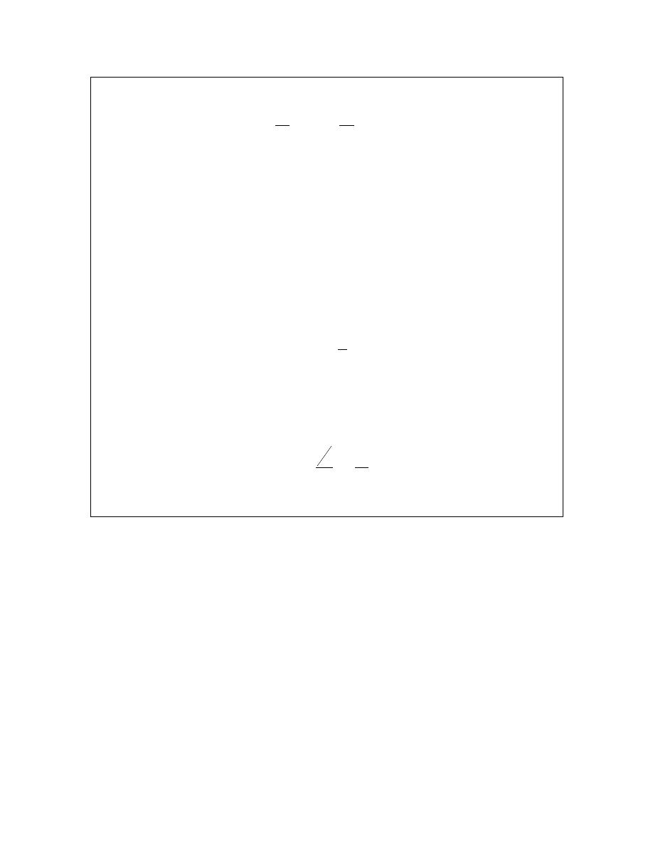
Calculus I

Now, recall that we have the following notational way of writing the derivative.

( )

(

)

y x

′

Using this we get the following,

xy′

Note that we dropped the

( )

on the y as it was only there to remind us that the y was a function

of x and now that we’ve taken the derivative it’s no longer really needed. We just wanted it in the
equation to recognize the product rule when we took the derivative.

So, let’s now recall just what were we after. We were after the derivative,

y′

, and notice that

there is now a

y′

in the equation. So, to get the derivative all that we need to do is solve the

equation for

y′

′ = −

There it is. Using the second solution technique this is our answer. This is not what we got from
the first solution however. Or at least it doesn’t look like the same derivative that we got from the
first solution. Recall however, that we really do know what y is in terms of x and if we plug that
in we will get,

′ = −

= −

which is what we got from the first solution. Regardless of the solution technique used we should
get the same derivative.

The process that we used in the second solution to the previous example is called implicit
differentiation and that is the subject of this section. In the previous example we were able to
just solve for y and avoid implicit differentiation. However, in the remainder of the examples in
this section we either won’t be able to solve for y or, as we’ll see in one of the examples below,
the answer will not be in a form that we can deal with.

In the second solution above we replaced the y with

( )

y x

and then did the derivative. Recall

that we did this to remind us that y is in fact a function of x. We’ll be doing this quite a bit in

these problems, although we rarely actually write

( )

y x

. So, before we actually work anymore

implicit differentiation problems let’s do a quick set of “simple” derivatives that will hopefully

help us with doing derivatives of functions that also contain a

( )

y x

http://tutorial.math.lamar.edu/terms.aspx

Calculus I

Example 2

Differentiate each of the following.

(a)

(

)

−

( )

f x









( )

y x









[

Solution

]

(b)

(

)

sin 3 6x

−

( )

(

)

sin y x

[

Solution

]

(c)

−

( )

y x

[

Solution

]

Solution
These are written a little differently from what we’re used to seeing here. This is because we
want to match up these problems with what we’ll be doing in this section. Also, each of these
parts has several functions to differentiate starting with a specific function followed by a general
function. This again, is to help us with some specific parts of the implicit differentiation process
that we’ll be doing.

(a)

(

)

−

( )

f x









( )

y x









With the first function here we’re being asked to do the following,

(

)

(

) (

)

5 5





−









and this is just the chain rule. We differentiated the outside function (the exponent of 5) and then
multiplied that by the derivative of the inside function (the stuff inside the parenthesis).

For the second function we’re going to do basically the same thing. We’re going to need to use
the chain rule. The outside function is still the exponent of 5 while the inside function this time is

simply

( )

f x

. We don’t have a specific function here, but that doesn’t mean that we can’t at

least write down the chain rule for this function. Here is the derivative for this function,

( )

f x

′

















We don’t actually know what

( )

f x

is so when we do the derivative of the inside function all we

can do is write down notation for the derivative, i.e.

( )

′

With the final function here we simply replaced the f in the second function with a y since most
of our work in this section will involve y’s instead of f’s. Outside of that this function is identical
to the second. So, the derivative is,

( )

y x

′

















[

Return to Problems

]

(b)

(

)

sin 3 6x

−

( )

(

)

sin y x

The first function to differentiate here is just a quick chain rule problem again so here is it’s
derivative,

http://tutorial.math.lamar.edu/terms.aspx

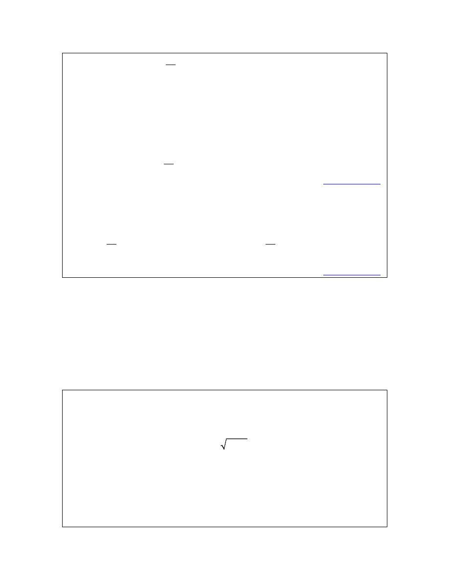
Calculus I

(

)

(

)

sin 3 6

6 cos 3 6

−

= −

−









For the second function we didn’t bother this time with using

( )

f x

and just jumped straight to

( )

y x

for the general version. This is still just a general version of what we did for the first

function. The outside function is still the sine and the inside is given by

( )

y x

and while we

don’t have a formula for

( )

y x

and so we can’t actually take its derivative we do have a notation

for its derivative. Here is the derivative for this function,

( )

(

)

( )

(

)

sin

cos

y x





′





[

Return to Problems

]

(c)

−

( )

y x

In this part we’ll just give the answers for each and leave out the explanation that we had in the
first two parts.

(

)

(

)

( )

y x

−

′

−

[

Return to Problems

]

So, in this set of examples we were just doing some chain rule problems where the inside function

was

( )

y x

instead of a specific function. This kind of derivative shows up all the time in doing

implicit differentiation so we need to make sure that we can do them. Also note that we only did
this for three kinds of functions but there are many more kinds of functions that we could have
used here.

So, it’s now time to do our first problem where implicit differentiation is required, unlike the first
example where we could actually avoid implicit differentiation by solving for y.

Example 3

Find

y′

for the following function.

Solution
Now, this is just a circle and we can solve for y which would give,

= ±

−

Prior to starting this problem we stated that we had to do implicit differentiation here because we
couldn’t just solve for y and yet that’s what we just did. So, why can’t we use “normal”
differentiation here? The problem is the “

”. With this in the “solution” for y we see that y is in

fact two different functions. Which should we use? Should we use both? We only want a single
function for the derivative and at best we have two functions here.

http://tutorial.math.lamar.edu/terms.aspx

Calculus I

So, in this example we really are going to need to do implicit differentiation so we can avoid this.
In this example we’ll do the same thing we did in the first example and remind ourselves that y is

really a function of x and write y as

( )

y x

. Once we’ve done this all we need to do is

differentiate each term with respect to x.

( )

(

)

( )

y x









As with the first example the right side is easy. The left side is also pretty easy since all we need
to do is take the derivative of each term and note that the second term will be similar the part (a)
of the second example. All we need to do for the second term is use the chain rule.

After taking the derivative we have,

( )

y x

′









At this point we can drop the

( )

part as it was only in the problem to help with the

differentiation process. The final step is to simply solve the resulting equation for

y′

′

′ = −

Unlike the first example we can’t just plug in for y since we wouldn’t know which of the two
functions to use. Most answers from implicit differentiation will involve both x and y so don’t get
excited about that when it happens.

As always, we can’t forget our interpretations of derivatives.

Example 4

Find the equation of the tangent line to

at the point

(

)

Solution
First note that unlike all the other tangent line problems we’ve done in previous sections we need
to be given both the x and the y values of the point. Notice as well that this point does lie on the
graph of the circle (you can check by plugging the points into the equation) and so it’s okay to
talk about the tangent line at this point.

Recall that to write down the tangent line we need is the slope of the tangent line and this is
nothing more than the derivative evaluated at the given point. We’ve got the derivative from the
previous example so as we need to do is plug in the given point.

http://tutorial.math.lamar.edu/terms.aspx

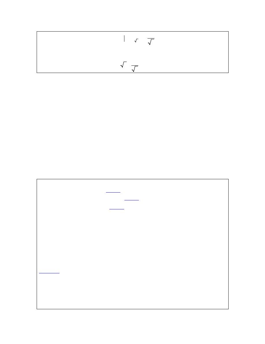
Calculus I

′

= −

The tangent line is then.

(

)

−

Now, let’s work some more examples. In the remaining examples we will no longer write

( )

y x

for y. This is just something that we were doing to remind ourselves that y is really a function of

x to help with the derivatives. Seeing the

( )

y x

reminded us that we needed to do the chain rule

on that portion of the problem. From this point on we’ll leave the y’s written as y’s and in our

head we’ll need to remember that they really are

( )

y x

and that we’ll need to do the chain rule.

There is an easy way to remember how to do the chain rule in these problems. The chain rule
really tells us to differentiate the function as we usually would, except we need to add on a
derivative of the inside function. In implicit differentiation this means that every time we are

differentiating a term with y in it the inside function is the y and we will need to add a

y′

onto the

term since that will be the derivative of the inside function.

Let’s see a couple of examples.

Example 5

Find

y′

for each of the following.

(a)

x y

[

Solution

]

(b)

( )

tan

sec

[

Solution

]

(c)

( )

−

[

Solution

]

Solution

(a)

x y

First differentiate both sides with respect to x and remember that each y is really

( )

y x

we just

aren’t going to write it that way anymore. This means that the first term on the left will be a
product rule.

We differentiated these kinds of functions involving y’s to a power with the chain rule in the

Example 2

above. Also, recall the discussion prior to the start of this problem. When doing this

kind of chain rule problem all that we need to do is differentiate the y’s as normal and then add on

y′

, which is nothing more than the derivative of the “inside function”.

Here is the differentiation of each side for this function.

x y

x y y

y y

′

+ =

http://tutorial.math.lamar.edu/terms.aspx

Calculus I

Now all that we need to do is solve for the derivative,

y′

. This is just basic solving algebra that

you are capable of doing. The main problem is that it’s liable to be messier than what you’re

used to doing. All we need to do is get all the terms with

y′

in them on one side and all the terms

without

y′

in them on the other. Then factor

y′

out of all the terms containing it and divide both

sides by the “coefficient” of the

y′

. Here is the solving work for this one,

(

)

x y

y y

x y y

x y

′

+ =

−

′

+ =

−

′ =

−

The algebra in these problems can be quite messy so be careful with that.

[

Return to Problems

]

(b)

( )

tan

sec

We’ve got two product rules to deal with this time. Here is the derivative of this function.

( )

( ) ( )

2 tan

sec

tan

y y

′

Notice the derivative tacked onto the secant! Again, this is just a chain rule problem similar to
the second part of Example 2 above.

Now, solve for the derivative.

( )

(

)

( ) ( )

( )

( ) ( )

( )

sec

tan

2 tan

sec

tan

2 tan

sec

′

= −

−

′ =

[

Return to Problems

]

(c)

( )

−

We’re going to need to be careful with this problem. We’ve got a couple chain rules that we’re
going to need to deal with here that are a little different from those that we’ve dealt with prior to
this problem.

In both the exponential and the logarithm we’ve got a “standard” chain rule in that there is
something other than just an x or y inside the exponential and logarithm. So, this means we’ll do
the chain rule as usual here and then when we do the derivative of the inside function for each
term we’ll have to deal with differentiating y’s.

Here is the derivative of this equation.

http://tutorial.math.lamar.edu/terms.aspx

Calculus I

(

)

2 3

xy y

′

−

In both of the chain rules note that the

y′

didn’t get tacked on until we actually differentiated the

y’s in that term.

Now we need to solve for the derivative and this is liable to be somewhat messy. In order to get

the

y′

on one side we’ll need to multiply the exponential through the parenthesis and break up

the quotient.

(

)

xy y

−

′

−

′

− −

′

−

′ =

Note that to make the derivative at least look a little nicer we converted all the fractions to
negative exponents.

[

Return to Problems

]

Okay, we’ve seen one application of implicit differentiation in the tangent line example above.
However, there is another application that we will be seeing in every problem in the next section.

In some cases we will have two (or more) functions all of which are functions of a third variable.

So, we might have

( )

x t

and

( )

y t

, for example and in these cases we will be differentiating

with respect to t. This is just implicit differentiation like we did in the previous examples, but
there is a difference however.

In the previous examples we have functions involving x’s and y’s and thinking of y as

( )

y x

. In

these problems we differentiated with respect to x and so when faced with x’s in the function we
differentiated as normal and when faced with y’s we differentiated as normal except we then

added a

y′

onto that term because we were really doing a chain rule.

In the new example we want to look at we’re assuming that

( )

x t

and that

( )

y t

and

differentiating with respect to t. This means that every time we are faced with an x or a y we’ll be
doing the chain rule. This in turn means that when we differentiate an x we will need to add on

x′

and whenever we differentiate a y we will add on a

y′

http://tutorial.math.lamar.edu/terms.aspx

Calculus I

These new types of problems are really the same kind of problem we’ve been doing in this
section. They are just expanded out a little to include more than one function that will require a
chain rule.

Let’s take a look at an example of this kind of problem.

Example 6

Assume that

( )

x t

and

( )

y t

and differentiate the following equation with

respect to t.

( )

cos 5

x y

−

Solution
So, just differentiate as normal and add on an appropriate derivative at each step. Note as well
that the first term will be a product rule since both x and y are functions of t.

( )

5 sin 5

x x y

x y y

−

′

−

There really isn’t all that much to this problem. Since there are two derivatives in the problem we
won’t be bothering to solve for one of them. When we do this kind of problem in the next section
the problem will imply which one we need to solve for.

At this point there doesn’t seem be any real reason for doing this kind of problem, but as we’ll see
in the next section every problem that we’ll be doing there will involve this kind of implicit
differentiation.

http://tutorial.math.lamar.edu/terms.aspx

Calculus I

Related Rates

In this section we are going to look at an application of implicit differentiation. Most of the
applications of derivatives are in the next chapter however there are a couple of reasons for
placing it in this chapter as opposed to putting it into the next chapter with the other applications.
The first reason is that it’s an application of implicit differentiation and so putting it right after
that section means that we won’t have forgotten how to do implicit differentiation. The other
reason is simply that after doing all these derivatives we need to be reminded that there really are
actual applications to derivatives. Sometimes it is easy to forget there really is a reason that we’re
spending all this time on derivatives.

For these related rates problems it’s usually best to just jump right into some problems and see
how they work.

Example 1

Air is being pumped into a spherical balloon at a rate of 5 cm

/min. Determine the

rate at which the radius of the balloon is increasing when the diameter of the balloon is 20 cm.

Solution
The first thing that we’ll need to do here is to identify what information that we’ve been given
and what we want to find. Before we do that let’s notice that both the volume of the balloon and

the radius of the balloon will vary with time and so are really functions of time, i.e.

( )

V t

and

( )

r t

We know that air is being pumped into the balloon at a rate of 5 cm

/min. This is the rate at

which the volume is increasing. Recall that rates of change are nothing more than derivatives and
so we know that,

( )

V t

′

We want to determine the rate at which the radius is changing. Again, rates are derivatives and so
it looks like we want to determine,

( )

when

10 cm

r t

′

= =

Note that we needed to convert the diameter to a radius.

Now that we’ve identified what we have been given and what we want to find we need to relate
these two quantities to each other. In this case we can relate the volume and the radius with the
formula for the volume of a sphere.

( )

V t

r t









As in the previous section when we looked at implicit differentiation, we will typically not use

the

( )

part of things in the formulas, but since this is the first time through one of these we will

http://tutorial.math.lamar.edu/terms.aspx

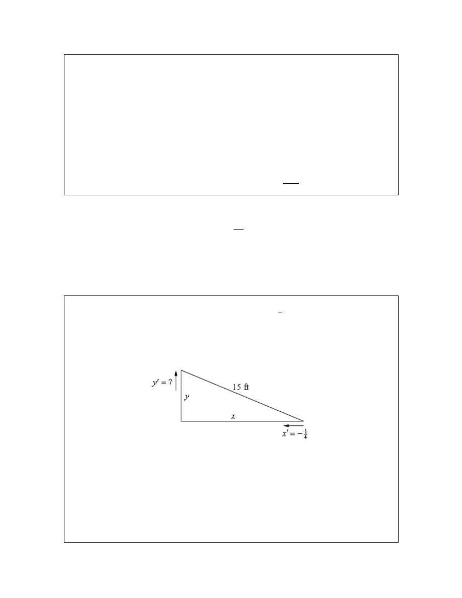
Calculus I

do that to remind ourselves that they are really functions of t.

Now we don’t really want a relationship between the volume and the radius. What we really
want is a relationship between their derivatives. We can do this by differentiating both sides with
respect to t. In other words, we will need to do implicit differentiation on the above formula.
Doing this gives,

r r

′

Note that at this point we went ahead and dropped the

( )

from each of the terms. Now all that

we need to do is plug in what we know and solve for what we want to find.

( )

cm/min

′

⇒

We can get the units of the derivative by recalling that,

′ =

The units of the derivative will be the units of the numerator (cm in the previous example)
divided by the units of the denominator (min in the previous example).

Let’s work some more examples.

Example 2

A 15 foot ladder is resting against the wall. The bottom is initially 10 feet away

from the wall and is being pushed towards the wall at a rate of

1
4

ft/sec. How fast is the top of the

ladder moving up the wall 12 seconds after we start pushing?

Solution
The first thing to do in this case is to sketch picture that shows us what is going on.

We’ve defined the distance of the bottom of the ladder from the wall to be x and the distance of
the top of the ladder from the floor to be y. Note as well that these are changing with time and so

we really should write

( )

x t

and

( )

y t

. However, as is often the case with related rates/implicit

differentiation problems we don’t write the

( )

part just try to remember this in our heads as we

proceed with the problem.

Next we need to identify what we know and what we want to find. We know that the rate at
which the bottom of the ladder is moving towards the wall. This is,

http://tutorial.math.lamar.edu/terms.aspx

Calculus I

x′

= −

Note as well that the rate is negative since the distance from the wall, x, is decreasing. We always
need to be careful with signs with these problems.

We want to find the rate at which the top of the ladder is moving away from the floor. This is

y′

Note as well that this quantity should be positive since y will be increasing.

As with the first example we first need a relationship between x and y. We can get this using
Pythagorean theorem.

( )

225

All that we need to do at this point is to differentiate both sides with respect to t, remembering
that x and y are really functions of t and so we’ll need to do implicit differentiation. Doing this
gives an equation that shows the relationship between the derivatives.

′

(1)

Next, let’s see which of the various parts of this equation that we know and what we need to find.

We know

x′

and are being asked to determine

y′

so it’s okay that we don’t know that.

However, we still need to determine x and y.

Determining x and y is actually fairly simple. We know that initially

and the end is being

pushed in towards the wall at a rate of

1
4

ft/sec and that we are interested in what has happened

after 12 seconds. We know that,

( )

distance

rate time

 

 

 

So, the end of the ladder has been pushed in 3 feet and so after 12 seconds we must have

Note that we could have computed this in one step as follows,

( )

−

To find y (after 12 seconds) all that we need to do is reuse the Pythagorean Theorem with the
values of x that we just found above.

225

225 49

176

−

Now all that we need to do is plug into (1) and solve for

y′

http://tutorial.math.lamar.edu/terms.aspx

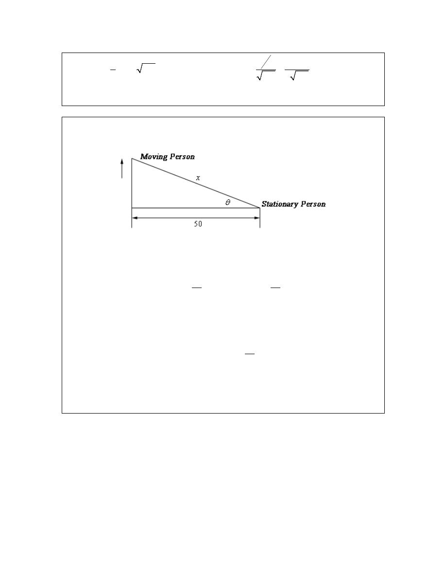
Calculus I

( )

(

)

2 7

176

0.1319 ft/sec

176

4 176





′

−

⇒









Notice that we got the correct sign for

y′

. If we’d gotten a negative then we’d have known that

we had made a mistake and we could go back and look for it.

Example 3

Two people are 50 feet apart. One of them starts walking north at a rate so that the

angle shown in the diagram below is changing at a constant rate of 0.01 rad/min. At what rate is
distance between the two people changing when

0.5

radians?

Solution
This example is not as tricky as it might at first appear. Let’s call the distance between them at
any point in time x as noted above. We can then relate all the known quantities by one of two trig
formulas.

cos

sec

We want to find

x′

and we could find x if we wanted to at the point in question using cosine since

we also know the angle at that point in time. However, if we use the second formula we won’t
need to know x as you’ll see. So, let’s differentiate that formula.

sec tan

θ θ

′

′ =

As noted, there are no x’s in this formula. We want to determine

x′

and we know that

0.5

and

0.01

′ =

(do you agree with it being positive?). So, just plug in and solve.

( )(

) ( ) ( )

50 0.01 sec 0.5 tan 0.5

0.311254 ft / min

′

⇒

So far we we’ve seen three related rates problems. While each one was worked in a very
different manner the process was essentially the same in each. In each problem we identified
what we were given and what we wanted to find. We next wrote down a relationship between all
the various quantities and used implicit differentiation to arrive at a relationship between the
various derivatives in the problem. Finally, we plugged into the equation to find the value we
were after.

So, in a general sense each problem was worked in pretty much the same manner. The only real
difference between them was coming up with the relationship between the known and unknown

http://tutorial.math.lamar.edu/terms.aspx

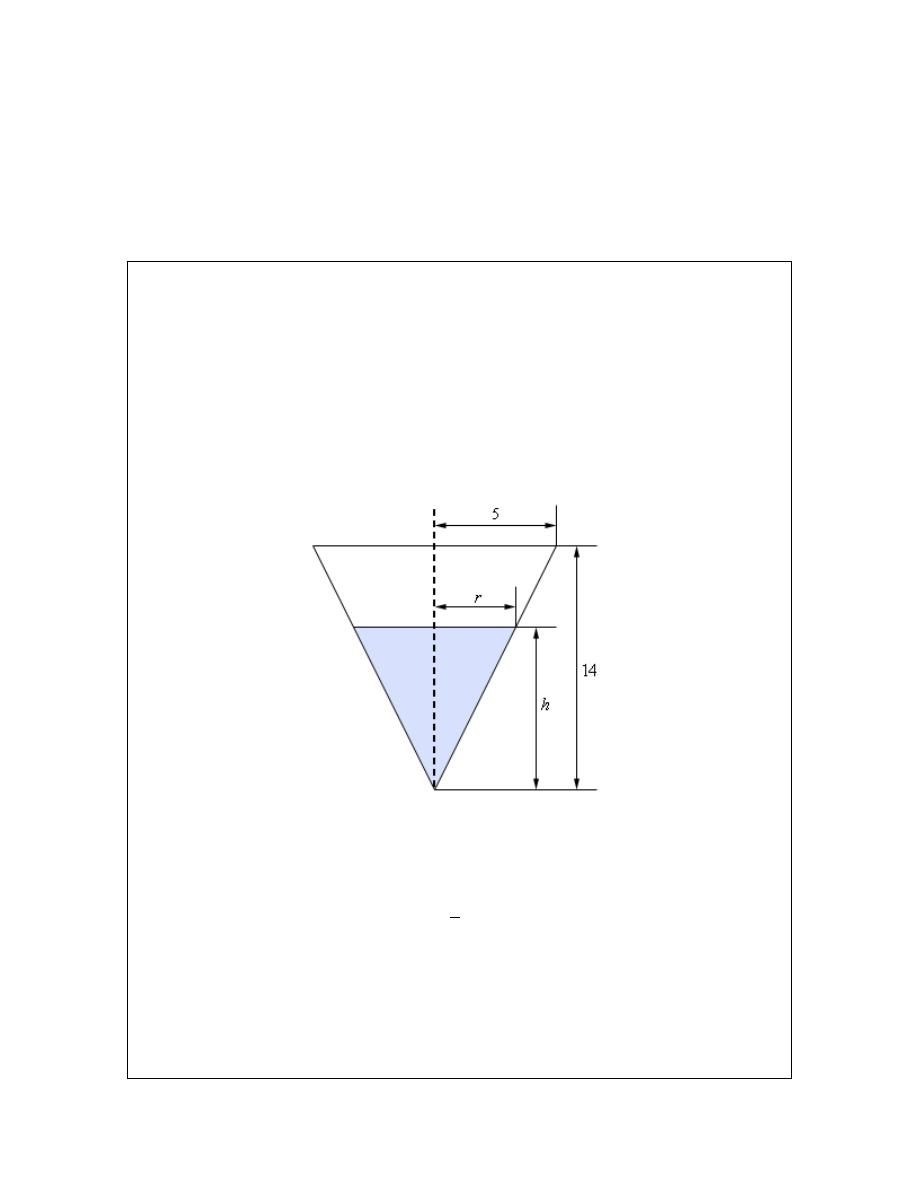
Calculus I

quantities. This is often the hardest part of the problem. In many problems the best way to come
up with the relationship is to sketch a diagram that shows the situation. This often seems like a
silly step, but can make all the difference in whether we can find the relationship or not.

Let’s work another problem that uses some different ideas and shows some of the different kinds
of things that can show up in related rates problems.

Example 4

A tank of water in the shape of a cone is leaking water at a constant rate of

2 ft /hour

. The base radius of the tank is 5 ft and the height of the tank is 14 ft.

(a) At what rate is the depth of the water in the tank changing when the depth of the

water is 6 ft?

(b) At what rate is the radius of the top of the water in the tank changing when the depth

of the water is 6 ft?

Solution
Okay, we should probably start off with a quick sketch (probably not to scale) of what is going on
here.

As we can see, the water in the tank actually forms a smaller cone with the same central angle as
the tank itself. The radius of the “water” cone at any time is given by r and the height of the
“water” cone at any time is given by h. The volume of water in the tank at any time t is given by,

r h

and we’ve been given that

V ′

= −

(a) At what rate is the depth of the water in the tank changing when the depth of the water
is 6 ft?

For this part we need to determine

h′

when

and now we have a problem. The only

http://tutorial.math.lamar.edu/terms.aspx

Calculus I

formula that we’ve got that will relate the volume to the height also includes the radius and so if
we were to differentiate this with respect to t we would get,

rr h

r h

′

So, in this equation we know

V ′

and h and want to find

h′

, but we don’t know r and

r′

. As

we’ll see finding r isn’t too bad, but we just don’t have enough information, at this point, that will

allow us to find

r′

and

h′

simultaneously.

To fix this we’ll need to eliminate the r from the volume formula in some way. This is actually
easier than it might at first look. If we go back to our sketch above and look at just the right half
of the tank we see that we have two similar triangles and when we say similar we mean similar in
the geometric sense. Recall that two triangles are called similar if their angles are identical,
which is the case here. When we have two similar triangles then ratios of any two sides will be
equal. For our set this means that we have,

⇒

If we take this and plug it into our volume formula we have,

588

r h













This gives us a volume formula that only involved the volume and the height of the water. Note
however that this volume formula is only valid for our cone, so don’t be tempted to use it for
other cones! If we now differentiate this we have,

196

h h

′

At this point all we need to do is plug in what we know and solve for

h′

( )

0.1386

196

225

−

′

− =

⇒

= −

So, it looks like the height is decreasing at a rate of 0.1386 ft/hr.

(b) At what rate is the radius of the top of the water in the tank changing when the depth of
the water is 6 ft?

In this case we are asking for

r′

and there is an easy way to do this part and a difficult (well,

more difficult than the easy way anyway….) way to do it. The “difficult” way is to redo the work
in part (a) above only this time use,

⇒

http://tutorial.math.lamar.edu/terms.aspx

Calculus I

to get the volume in terms of V and r and then proceed as before.

That’s not terribly difficult, but it is more work that we need to so. Recall from the first part that
we have,

′

⇒

So, as we can see if we take the relationship that relates r and h that we used in the first part and

differentiate it we get a relationship between

r′

and

h′

. At this point all we need to do here is

use the result from the first part to get,

0.04951

14 225

−





′ =

= −









Much easier that redoing all of the first part. Note however, that we were only able to do this the

“easier” way because it was asking for

r′

at exactly the same time that we asked for

h′

in the

first part. If we hadn’t been using the same time then we would have had no choice but to do this
the “difficult” way.

In the second part of the previous problem we saw an important idea in dealing with related rates.
In order to find the asked for rate all we need is an equation that relates the rate we’re looking for
to a rate that we already know. Sometimes there are multiple equations that we can use and
sometimes one will be easier than another.

Also, this problem showed us that we will often have an equation that contains more variables
that we have information about and so, in these cases, we will need to eliminate one (or more) of
the variables. In this problem we eliminated the extra variable using the idea of similar triangles.
This will not always be how we do this, but many of these problems do use similar triangles so
make sure you can use that idea.

Let’s work some more problems.

Example 5

A trough of water is 8 meters deep and its ends are in the shape of isosceles

triangles whose width is 5 meters and height is 2 meters. If water is being pumped in at a

constant rate of

6 m /sec

. At what rate is the height of the water changing when the water has a

height of 120 cm?

Solution
Note that an isosceles triangle is just a triangle in which two of the sides are the same length. In
our case sides of the tank have the same length.

We definitely need a sketch of this situation to get us going here so here. A sketch of the trough
is shown below.

http://tutorial.math.lamar.edu/terms.aspx

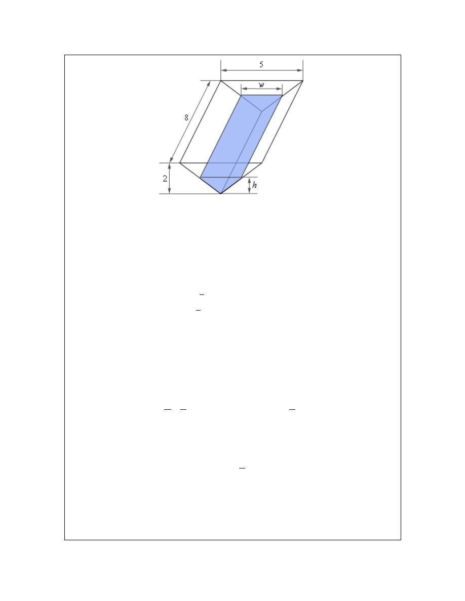
Calculus I

Now, in this problem we know that

6 m /sec

V ′

and we want to determine

h′

when

1.2 m

. Note that because

V ′

is in terms of meters we need to convert h into meters as well.

So, we need an equation that will relate these two quantities and the volume of the tank will do it.

The volume of this kind of tank is simple to compute. The volume is the area of the end times the
depth. For our case the volume of the water in the tank is,

(

)(

)

(

)

(

)

( )

1
2

Area of End

depth

base height

depth

=
=

As with the previous example we’ve got an extra quantity here, w, that is also changing with time
and so we need to eliminate it from the problem. To do this we’ll again make use of the idea of
similar triangles. If we look at the end of the tank we’ll see that we again have two similar
triangles. One for the tank itself and one formed by the water in the tank. Again, remember that
with similar triangles ratios of sides must be equal. In our case we’ll use,

⇒

Plugging this into the volume gives a formula for the volume (and only for this tank) that only
involved the height of the water.













We can now differentiate this to get,

′

Finally, all we need to do is plug in and solve for

h′

http://tutorial.math.lamar.edu/terms.aspx

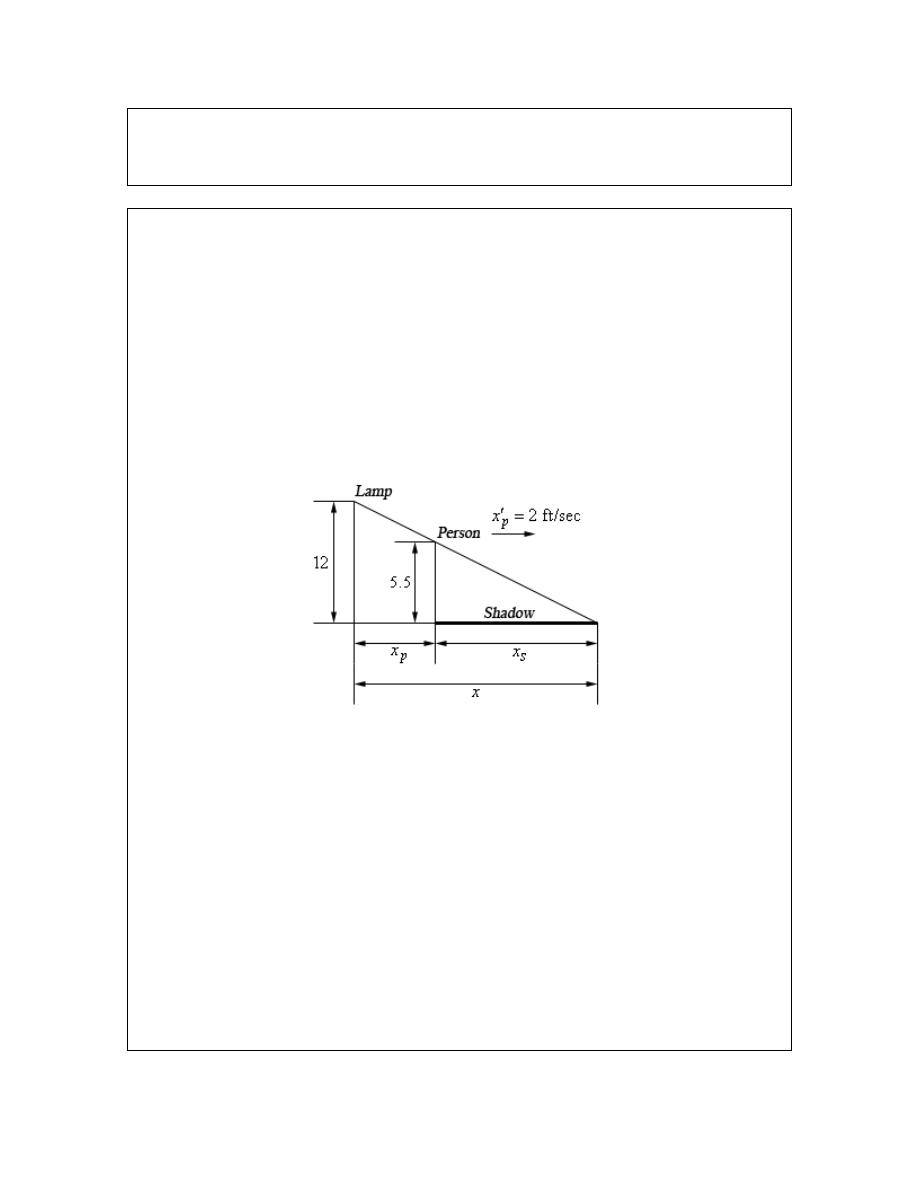
Calculus I

( )

20 1.2

0.25 m/sec

′

⇒

So, the height of the water is rising at a rate of 0.25 m/sec.

Example 6

A light is on the top of a 12 ft tall pole and a 5ft 6in tall person is walking away

from the pole at a rate of 2 ft/sec.

(a) At what rate is the tip of the shadow moving away from the pole when the person is

25 ft from the pole?

(b) At what rate is the tip of the shadow moving away from the person when the person is

25 ft from the pole?

Solution
We’ll definitely need a sketch of this situation to get us started here. The tip of the shadow is
defined by the rays of light just getting past the person and so we can form the following set of
similar triangles.

Here x is the distance of the tip of the shadow from the pole,

is the distance of the person

from the pole and

is the length of the shadow. Also note that we converted the persons height

over to 5.5 feet since all the other measurements are in feet.

(a) At what rate is the tip of the shadow moving away from the pole when the person is 25 ft
from the pole?

In this case we want to determine

x′

when

given that

x′

The equation we’ll need here is,

but we’ll need to eliminate

from the equation in order to get an answer. To do this we can

again make use of the fact that the two triangles are similar to get,

http://tutorial.math.lamar.edu/terms.aspx

Calculus I

5.5

Note :

We’ll need to solve this for

(

)

Our equation then becomes,

Now all that we need to do is differentiate this, plug in and solve for

x′

( )

3.6923 ft/sec

′

⇒

The tip of the shadow is then moving away from the pole at a rate of 3.6923 ft/sec. Notice as

well that we never actually had to use the fact that

for this problem. That will happen

on rare occasions.

(b) At what rate is the tip of the shadow moving away from the person when the person is
25 ft from the pole?

This part is actually quite simple if we have the answer from (a) in hand, which we do of course.

In this case we know that

represents the length of the shadow, or the distance of the tip of the

shadow from the person so it looks like we want to determine

x′

when

Again, we can use

, however unlike the first part we now know that

x′

and

3.6923 ft/sec

x′

so in this case all we need to do is differentiate the equation and plug in for

all the known quantities.

3.6923

1.6923 ft/sec

′

= +

The tip of the shadow is then moving away from the person at a rate of 1.6923 ft/sec.

http://tutorial.math.lamar.edu/terms.aspx

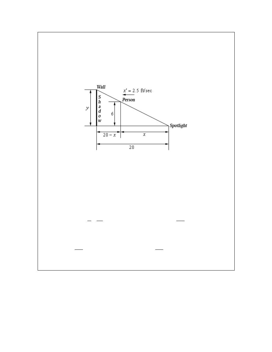
Calculus I

Example 7

A spot light is on the ground 20 ft away from a wall and a 6 ft tall person is walking

towards the wall at a rate of 2.5 ft/sec. How fast is the height of the shadow changing when the
person is 8 feet from the wall? Is the shadow increasing or decreasing in height at this time?

Solution
Let’s start off with a sketch of this situation and the sketch here will be similar to that of the
previous problem. The top of the shadow will be defined by the light rays going over the head of
the person and so we again get yet another set of similar triangles.

In this case we want to determine

y′

when the person is 8 ft from wall or

12 ft

. Also, if the

person is moving towards the wall at 2.5 ft/sec then the person must be moving away from the

spotlight at 2.5 ft/sec and so we also know that

2.5

x′

In all the previous problems that used similar triangles we used the similar triangles to eliminate
one of the variables from the equation we were working with. In this case however, we can get
the equation that relates x and y directly from the two similar triangles. In this case the equation
we’re going to work with is,

120

⇒

Now all that we need to do is differentiate and plug values into solve to get

y′

( )

120

2.5

2.0833 ft/sec

′

= −

⇒

= −

The height of the shadow is then decreasing at a rate of 2.0833 ft/sec.

Okay, we’ve worked quite a few problems now that involved similar triangles in one form or
another so make sure you can do these kinds of problems.

It’s now time to do a problem that while similar to some of the problems we’ve done to this point
is also sufficiently different that it can cause problems until you’ve seen how to do it.

http://tutorial.math.lamar.edu/terms.aspx

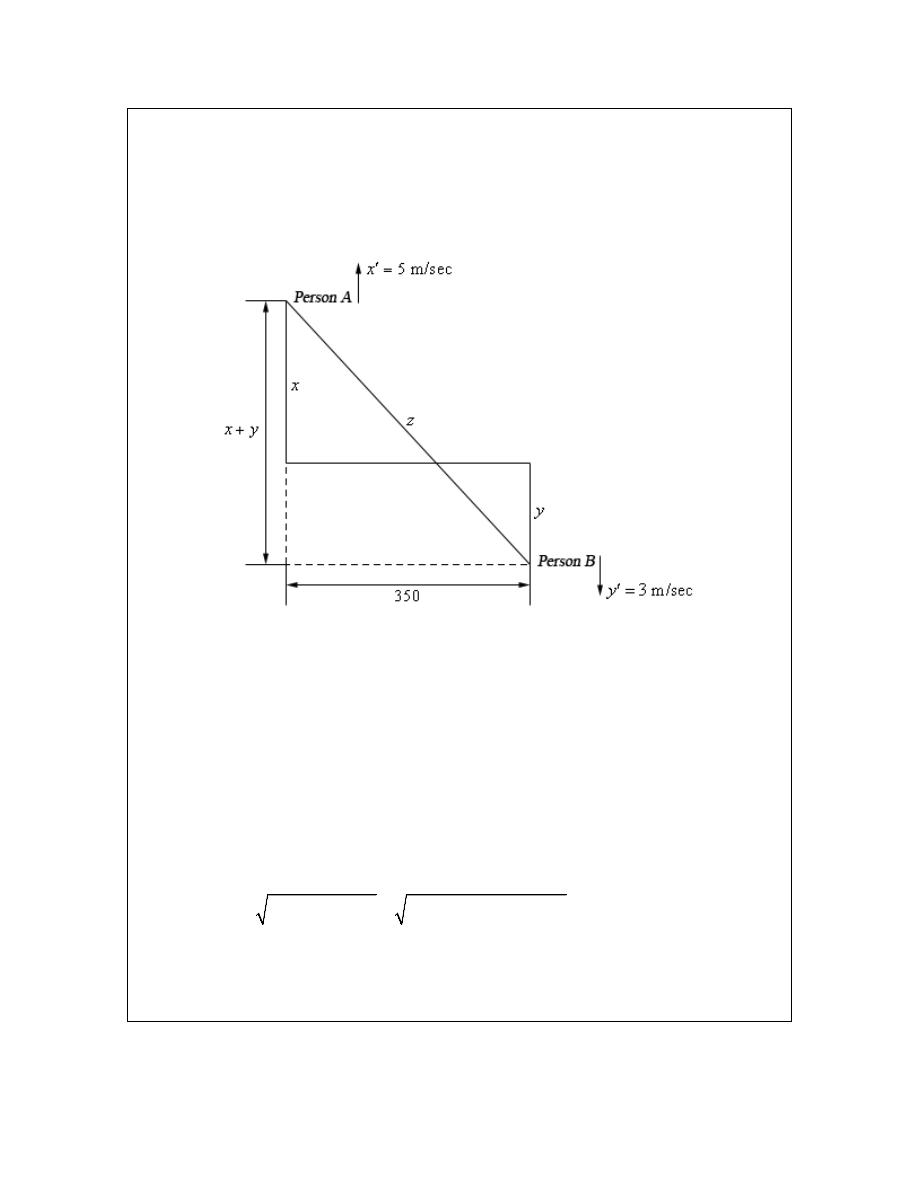
Calculus I

Example 8

Two people on bikes are separated by 350 meters. Person A starts riding north at a

rate of 5 m/sec and 7 minutes later Person B starts riding south at 3 m/sec. At what rate is the
distance separating the two people changing 25 minutes after Person A starts riding?

Solution
There is a lot to digest here with this problem. Let’s start off with a sketch of the situation.

Now we are after

z′

and we know that

x′

and

y′

. We want to know

z′

after Person A

had been riding for 25 minutes and Person B has been riding for

25 7

− =

minutes. After

converting these times to seconds (because our rates are all in m/sec) this means that at the time
we’re interested in each of the bike riders has rode,

(

)

(

)

5 25 60

7500 m

3 18 60

3240 m

Next, the Pythagorean theorem tells us that,

(

)

350

(2)

Therefore, 25 minutes after Person A starts riding the two bike riders are

(

)

(

)

350

7500 3240

350

10745.7015 m

apart.

To determine the rate at which the two riders are moving apart all we need to do then is

differentiate (2) and plug in all the quantities that we know to find

z′

http://tutorial.math.lamar.edu/terms.aspx

Calculus I

(

)(

)

(

)

(

)(

)

2 10745.7015

2 7500 3240 5 3

7.9958 m/sec

′

′ =

So, the two riders are moving apart at a rate of 7.9958 m/sec.

Every problem that we’ve worked to this point has come down to needing a geometric formula
and we should probably work a quick problem that is not geometric in nature.

Example 9

Suppose that we have two resistors connected in parallel with resistances

and

measured in ohms (

Ω

). The total resistance, R, is then given by,

Suppose that

is increasing at a rate of 0.4

Ω

/min and

is decreasing at a rate of

0.7

Ω

/min. At what rate is R changing when

Ω

and

105

Ω

Solution
Okay, unlike the previous problems there really isn’t a whole lot to do here. First, let’s note that

we’re looking for

R′

and that we know

0.4

R′

and

0.7

R′

= −

. Be careful with the signs

here.

Also, since we’ll eventually need it let’s determine R at the time we’re interested in.

1680

45.4054

105

1680

⇒

Ω

Next we need to differentiate the equation given in the problem statement.

( )

′

−

= −

−









′









Finally, all we need to do is plug into this and do some quick computations.

(

)

( )

(

)

45.4054

0.4

0.7

0.002045

105





′ =

−

= −









So, it looks like R is decreasing at a rate of 0.002045

Ω

/min.

http://tutorial.math.lamar.edu/terms.aspx

Calculus I

We’ve seen quite a few related rates problems in this section that cover a wide variety of possible
problems. There are still many more different kinds of related rates problems out there in the
world, but the ones that we’ve worked here should give you a pretty good idea on how to at least
start most of the problems that you’re liable to run into.

http://tutorial.math.lamar.edu/terms.aspx

Calculus I

Higher Order Derivatives

Let’s start this section with the following function.

( )

f x

−

By this point we should be able to differentiate this function without any problems. Doing this
we get,

( )

′

−

Now, this is a function and so it can be differentiated. Here is the notation that we’ll use for that,
as well as the derivative.

( )

(

)

′

′′

′

−

This is called the second derivative and

( )

′

is now called the first derivative.

Again, this is a function so we can differentiate it again. This will be called the third derivative.
Here is that derivative as well as the notation for the third derivative.

( )

(

)

x ′

′′′

′′

Continuing, we can differentiate again. This is called, oddly enough, the fourth derivative.
We’re also going to be changing notation at this point. We can keep adding on primes, but that
will get cumbersome after awhile.

( )

(

)

(4)

x ′

′′′

This process can continue but notice that we will get zero for all derivatives after this point. This
set of derivatives leads us to the following fact about the differentiation of polynomials.

Fact
If p(x) is a polynomial of degree n (i.e. the largest exponent in the polynomial) then,

( )

for 1

≥ +

We will need to be careful with the “non-prime” notation for derivatives. Consider each of the
following.

( )

f x

′′

= 







The presence of parenthesis in the exponent denotes differentiation while the absence of
parenthesis denotes exponentiation.

Collectively the second, third, fourth, etc. derivatives are called higher order derivatives.

http://tutorial.math.lamar.edu/terms.aspx

Calculus I

Let’s take a look at some examples of higher order derivatives.

Example 1

Find the first four derivatives for each of the following.

(a)

( )

R t

+ e

[

Solution

]

(b)

cos

[

Solution

]

(c)

( )

sin 3

ln 7

f y

−

[

Solution

]

Solution

(a)

( )

R t

+ e

There really isn’t a lot to do here other than do the derivatives.

( )
( )
( )
( )

(4)

6 2

R t

−

′

= +

′′

= −

′′′

= −

Notice that differentiating an exponential function is very simple. It doesn’t change with each
differentiation.

[

Return to Problems

]

(b)

cos

Again, let’s just do some derivatives.

( )

cos

sin

cos

sin

cos

′ = −

′′ = −

′′′ =

Note that cosine (and sine) will repeat every four derivatives. The other four trig functions will
not exhibit this behavior. You might want to take a few derivatives to convince yourself of this.

[

Return to Problems

]

(c)

( )

sin 3

ln 7

f y

−

In the previous two examples we saw some patterns in the differentiation of exponential
functions, cosines and sines. We need to be careful however since they only work if there is just
a t or an x in the argument. This is the point of this example. In this example we will need to use
the chain rule on each derivative.

http://tutorial.math.lamar.edu/terms.aspx

Calculus I

( )

3cos 3

9 sin 3

27 cos 3

81sin 3

−

′

−

+ =

−

′′

= −

−

′′′

= −

−

So, we can see with slightly more complicated arguments the patterns that we saw for exponential
functions, sines and cosines no longer completely hold.

[

Return to Problems

]

Let’s do a couple more examples to make a couple of points.

Example 2

Find the second derivative for each of the following functions.

(a)

( )

sec 5

Q t

[

Solution

]

(b)

( )

1 2w

g w

−

= e

[

Solution

]

(c)

( )

(

)

ln 1

f t

[

Solution

]

Solution

(a)

( )

sec 5

Q t

Here’s the first derivative.

( )

( ) ( )

5sec 5 tan 5

Q t

′

Notice that the second derivative will now require the product rule.

( )

( ) ( ) ( )

( )

25sec 5 tan 5 tan 5

25sec 5 sec

25sec 5 tan

25sec 5

Q t

′′

Notice that each successive derivative will require a product and/or chain rule and that as noted
above this will not end up returning back to just a secant after four (or another other number for
that matter) derivatives as sine and cosine will.

[

Return to Problems

]

(b)

( )

1 2w

g w

−

= e

Again, let’s start with the first derivative.

( )

1 2

g w

−

′

= −

As with the first example we will need the product rule for the second derivative.

( )

(

)

1 2

−

′′

= −

−

= −

[

Return to Problems

]

http://tutorial.math.lamar.edu/terms.aspx

Calculus I

(c)

( )

(

)

ln 1

f t

Same thing here.

( )

′

The second derivative this time will require the quotient rule.

( )

(

)

( )( )

(

)

(

)

2 1

2 2

−

′′

−

[

Return to Problems

]

As we saw in this last set of examples we will often need to use the product or quotient rule for
the higher order derivatives, even when the first derivative didn’t require these rules.

Let’s work one more example that will illustrate how to use implicit differentiation to find higher
order derivatives.

Example 3

Find

y′′

for

Solution
Okay, we know that in order to get the second derivative we need the first derivative and in order
to get that we’ll need to do implicit differentiation. Here is the work for that.

y y

′

′ = −

Now, this is the first derivative. We get the second derivative by differentiating this, which will
require implicit differentiation again.

(

)

( )

y y

xy y

′





′′ = −









′

−

= −

′

−

= −

′

−

= −

http://tutorial.math.lamar.edu/terms.aspx

Calculus I

This is fine as far as it goes. However, we would like there to be no derivatives in the answer.
We don’t, generally, mind having x’s and/or y’s in the answer when doing implicit differentiation,
but we really don’t like derivatives in the answer. We can get rid of the derivative however by
acknowledging that we know what the first derivative is and substituting this into the second
derivative equation. Doing this gives,

x y

−

′

−

′′ = −





−









= −

Now that we’ve found some higher order derivatives we should probably talk about an
interpretation of the second derivative.

If the position of an object is given by s(t) we know that the velocity is the first derivative of the
position.

( )

v t

s t

′

The acceleration of the object is the first derivative of the velocity, but since this is the first
derivative of the position function we can also think of the acceleration as the second derivative
of the position function.

( )

a t

v t

s t

′

′′

Alternate Notation
There is some alternate notation for higher order derivatives as well. Recall that there was a
fractional notation for the first derivative.

( )

′

We can extend this to higher order derivatives.

( )

d y

etc

′′

′′′

http://tutorial.math.lamar.edu/terms.aspx

Calculus I

Logarithmic Differentiation

There is one last topic to discuss in this section. Taking the derivatives of some complicated
functions can be simplified by using logarithms. This is called logarithmic differentiation.

It’s easiest to see how this works in an example.

Example 1

Differentiate the function.

(

)

1 10

−

Solution
Differentiating this function could be done with a product rule and a quotient rule. However, that
would be a fairly messy process. We can simplify things somewhat by taking logarithms of both
sides.

(

)

1 10













−





Of course, this isn’t really simpler. What we need to do is use the properties of logarithms to
expand the right side as follows.

( )

(

)

(

)

( )

(

)

(

)

ln 1 10

−

This doesn’t look all that simple. However, the differentiation process will be simpler. What we
need to do at this point is differentiate both sides with respect to x. Note that this is really

implicit

differentiation

(

)

( )

(

)

1 10

−

′

−

′

= +

−

To finish the problem all that we need to do is multiply both sides by y and the plug in for y since
we do know what that is.

(

)

1 10





′ =

−





−









−





−





−

http://tutorial.math.lamar.edu/terms.aspx

Calculus I

Depending upon the person, doing this would probably be slightly easier than doing both the
product and quotient rule. The answer is almost definitely simpler than what we would have
gotten using the product and quotient rule.

So, as the first example has shown we can use logarithmic differentiation to avoid using the
product rule and/or quotient rule.

We can also use logarithmic differentiation to differentiation functions in the form.

( )

(

)

( )

g x

f x

Let’s take a quick look at a simple example of this.

Example 2

Differentiate

Solution
We’ve seen two functions similar to this at this point.

( )

−

Neither of these two will work here since both require either the base or the exponent to be a
constant. In this case both the base and the exponent are variables and so we have no way to
differentiate this function using only known rules from previous sections.

With logarithmic differentiation we can do this however. First take the logarithm of both sides as
we did in the first example and use the logarithm properties to simplify things a little.

=
=

Differentiate both sides using implicit differentiation.

′

 

 

 

As with the first example multiply by y and substitute back in for y.

(

)

(

)

1 ln

′ =

Let’s take a look at a more complicated example of this.

http://tutorial.math.lamar.edu/terms.aspx

Calculus I

Example 3

Differentiate

(

)

( )

cos

1 3

= −

Solution

Now, this looks much more complicated than the previous example, but is in fact only
slightly more complicated. The process is pretty much identical so we first take the log
of both sides and then simplify the right side.

(

)

( )

( ) (

)

cos

ln 1 3

cos

ln 1 3





−





Next, do some implicit differentiation.

( ) (

)

( )

( ) (

)

( )

sin

ln 1 3

cos

sin

ln 1 3

cos

1 3

′

−

= −

−

= −

−

Finally, solve for

y′

and substitute back in for y.

( ) (

)

( )

(

)

( )

( ) (

)

( )

cos

sin

ln 1 3

cos

1 3

sin

ln 1 3

cos

1 3





′ = −

−





−









= − −

−





−





A messy answer but there it is.

We’ll close this section out with a quick recap of all the various ways we’ve seen of
differentiating functions with exponents. It is important to not get all of these confused.

( )
( )
( )
( )

(

)

This is a constant

Power Rule

Derivative of an exponential function

1 ln

Logarithmic Differentiation

−

It is sometimes easy to get these various functions confused and use the wrong rule for
differentiation. Always remember that each rule has very specific rules for where the variable
and constants must be. For example, the Power Rule requires that the base be a variable and the
exponent be a constant, while the exponential function requires exactly the opposite.

If you can keep straight all the rules you can’t go wrong with these.

http://tutorial.math.lamar.edu/terms.aspx

Calculus I

http://tutorial.math.lamar.edu/terms.aspx