CalcI_Limits_Solutions pdf - عبدالرحمن سهيل

CALCULUS I

Solutions to Practice Problems

Limits

Paul Dawkins

Calculus I

http://tutorial.math.lamar.edu/terms.aspx

Table of Contents

Preface ............................................................................................................................................ 2

Limits .............................................................................................................................................. 2

Rates of Change and Tangent Lines......................................................................................................... 2

The Limit ..................................................................................................................................................12

One-Sided Limits .....................................................................................................................................20

Limit Properties .......................................................................................................................................27

Computing Limits ....................................................................................................................................36

Infinite Limits ..........................................................................................................................................43

Limits At Infinity, Part I ...........................................................................................................................56

Limits At Infinity, Part II .........................................................................................................................68

Continuity .................................................................................................................................................75

The Definition of the Limit ......................................................................................................................90

Calculus I

http://tutorial.math.lamar.edu/terms.aspx

Preface

Here are the solutions to the practice problems for my Calculus I notes.  Some solutions will have
more or less detail than other solutions. The level of detail in each solution will depend up on
several issues. If the section is a review section, this mostly applies to problems in the first
chapter, there will probably not be as much detail to the solutions given that the problems really
should be review. As the difficulty level of the problems increases less detail will go into the
basics of the solution under the assumption that if you’ve reached the level of working the harder
problems then you will probably already understand the basics fairly well and won’t need all the
explanation.

This document was written with presentation on the web in mind. On the web most solutions are
broken down into steps and many of the steps have hints. Each hint on the web is given as a
popup however in this document they are listed prior to each step. Also, on the web each step can
be viewed individually by clicking on links while in this document they are all showing. Also,
there are liable to be some formatting parts in this document intended for help in generating the
web pages that haven’t been removed here.  These issues may make the solutions a little difficult
to follow at times, but they should still be readable.

Limits

Rates of Change and Tangent Lines

1. For the function

( ) (

)

f x

and the point P given by

= −

answer each of the

following questions.

(a) For the points Q given by the following values of x compute (accurate to at least 8

decimal places) the slope,

, of the secant line through points P and Q.

(i) -3.5 (ii) -3.1 (iii) -3.01 (iv) -3.001 (v) -3.0001
(vi) -2.5 (vii) -2.9 (viii) -2.99 (ix) -2.999 (x) -2.9999

(b) Use the information from (a) to estimate the slope of the tangent line to

( )

f x

= −

and write down the equation of the tangent line.

Calculus I

http://tutorial.math.lamar.edu/terms.aspx

(a) For the points Q given by the following values of x compute (accurate to at least 8 decimal

places) the slope,

, of the secant line through points P and Q.

(i) -3.5 (ii) -3.1 (iii) -3.01 (iv) -3.001 (v) -3.0001
(vi) -2.5 (vii) -2.9 (viii) -2.99 (ix) -2.999 (x) -2.9999

[Solution]
The first thing that we need to do is set up the formula for the slope of the secant lines. As
discussed in this section this is given by,

( )

(

)

f x

−

− −

Now, all we need to do is construct a table of the value of

for the given values of x. All of

the values in the table below are accurate to 8 decimal places, but in this case the values
terminated prior to 8 decimal places and so the “trailing” zeros are not shown.

-3.5

-7.5

-2.5

-4.5

-3.1

-6.3

-2.9

-5.7

-3.01

-6.03

-2.99

-5.97

-3.001

-6.003

-2.999

-5.997

-3.0001 -6.0003 -2.9999 -5.9997

(b) Use the information from (a) to estimate the slope of the tangent line to

( )

f x

= −

and

write down the equation of the tangent line.
[Solution]
From the table of values above we can see that the slope of the secant lines appears to be moving

towards a value of -6 from both sides of

= −

and so we can estimate that the slope of the

tangent line is :

= −

The equation of the tangent line is then,

( )

(

)

(

)

3 6

m x

− +

− −

= −

⇒

= − −

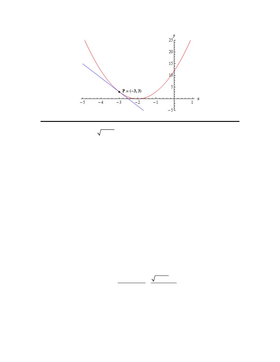
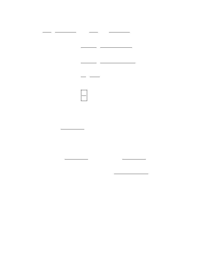
Here is a graph of the function and the tangent line.

Calculus I

http://tutorial.math.lamar.edu/terms.aspx

2. For the function

( )

g x

and the point P given by

answer each of the

following questions.

(a) For the points Q given by the following values of x compute (accurate to at least 8

decimal places) the slope,

, of the secant line through points P and Q.

(i) 2.5 (ii) 2.1 (iii) 2.01 (iv) 2.001 (v) 2.0001
(vi) 1.5 (vii) 1.9 (viii) 1.99 (ix) 1.999 (x) 1.9999

(b) Use the information from (a) to estimate the slope of the tangent line to

( )

g x

and write down the equation of the tangent line.

(a) For the points Q given by the following values of x compute (accurate to at least 8 decimal

places) the slope,

, of the secant line through points P and Q.

(i) 2.5 (ii) 2.1 (iii) 2.01 (iv) 2.001 (v) 2.0001
(vi) 1.5 (vii) 1.9 (viii) 1.99 (ix) 1.999 (x) 1.9999

[Solution]
The first thing that we need to do is set up the formula for the slope of the secant lines. As
discussed in this section this is given by,

( )

g x

−

+ −

−

Now, all we need to do is construct a table of the value of

for the given values of x. All of

the values in the table below are accurate to 8 decimal places.

Calculus I

http://tutorial.math.lamar.edu/terms.aspx

2.5

0.48528137 1.5

0.51668523

2.1

0.49691346 1.9

0.50316468

2.01

0.49968789 1.99

0.50031289

2.001

0.49996875 1.999

0.50003125

2.0001 0.49999688 1.9999 0.50000313

(b) Use the information from (a) to estimate the slope of the tangent line to

( )

g x

and

write down the equation of the tangent line.
[Solution]
From the table of values above we can see that the slope of the secant lines appears to be moving

towards a value of 0.5 from both sides of

and so we can estimate that the slope of the

tangent line is :

0.5

The equation of the tangent line is then,

( )

(

)

(

)

m x

−

= +

−

⇒

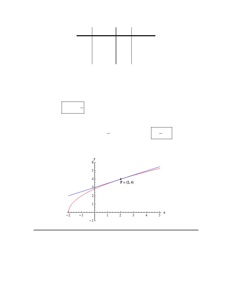
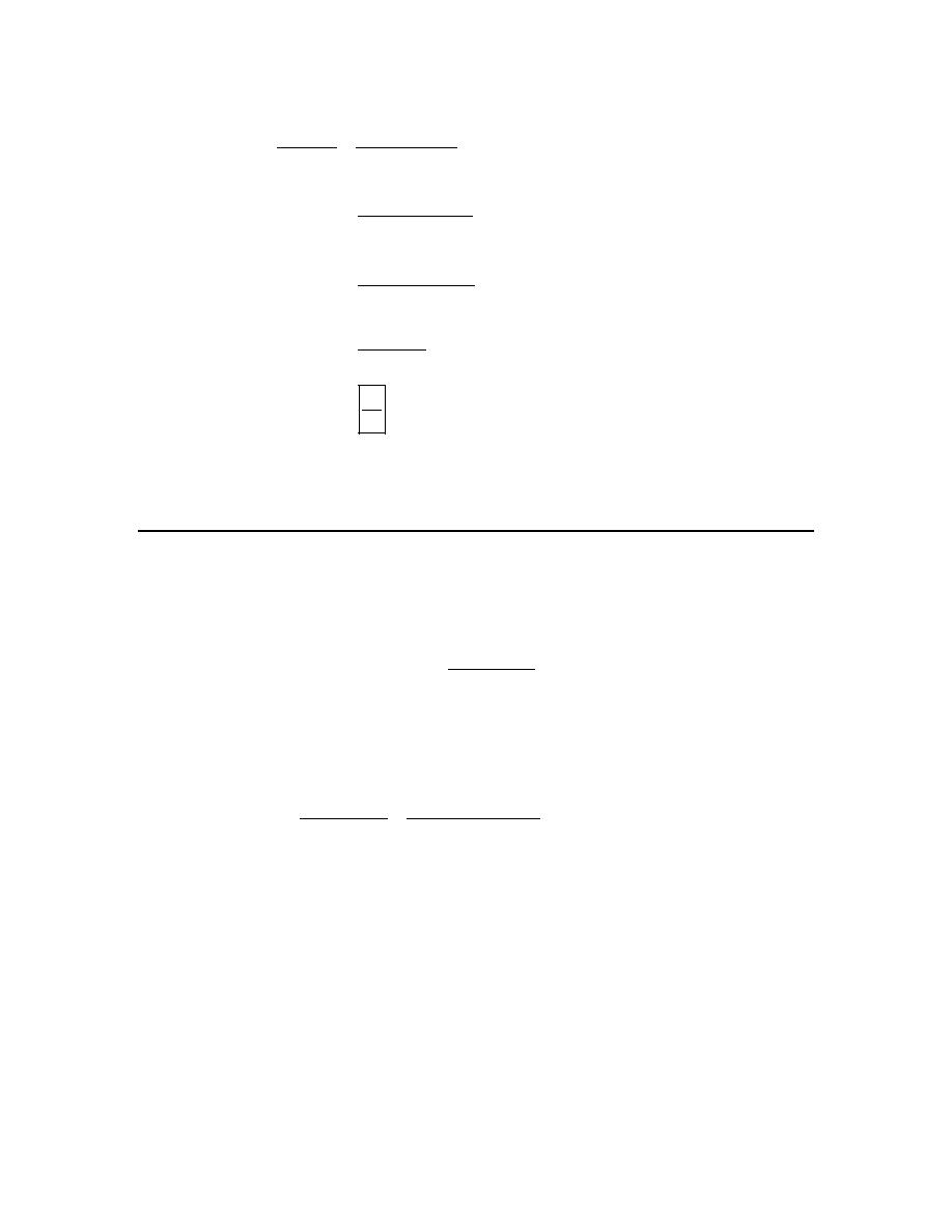
Here is a graph of the function and the tangent line.

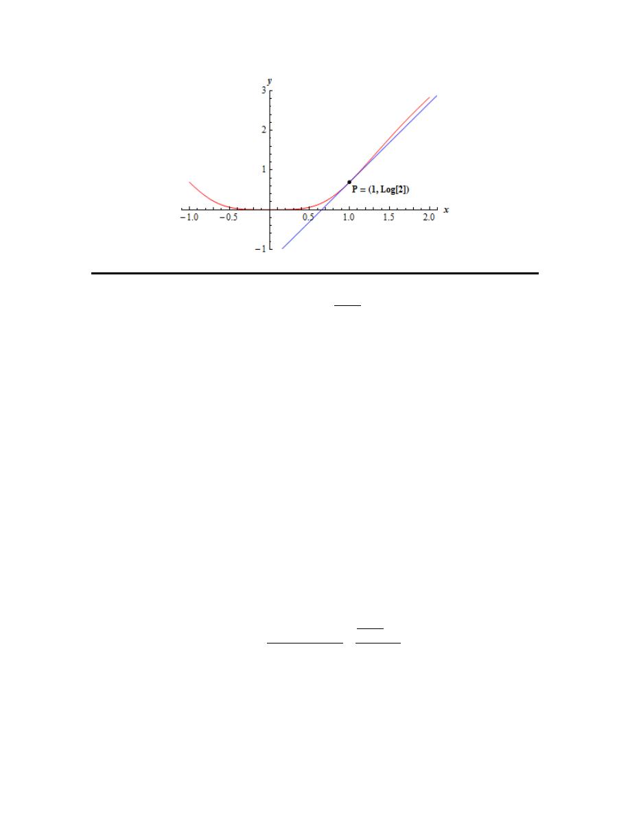
3. For the function

( )

(

)

ln 1

W x

and the point P given by

answer each of the

following questions.

(a) For the points Q given by the following values of x compute (accurate to at least 8

decimal places) the slope,

, of the secant line through points P and Q.

Calculus I

http://tutorial.math.lamar.edu/terms.aspx

(i) 1.5 (ii) 1.1 (iii) 1.01 (iv) 1.001 (v) 1.0001
(vi) 0.5 (vii) 0.9 (viii) 0.99 (ix) 0.999 (x) 0.9999

(b) Use the information from (a) to estimate the slope of the tangent line to

( )

W x

and write down the equation of the tangent line.

(a) For the points Q given by the following values of x compute (accurate to at least 8 decimal

places) the slope,

, of the secant line through points P and Q.

(i) 1.5 (ii) 1.1 (iii) 1.01 (iv) 1.001 (v) 1.0001
(vi) 0.5 (vii) 0.9 (viii) 0.99 (ix) 0.999 (x) 0.9999

[Solution]
The first thing that we need to do is set up the formula for the slope of the secant lines. As
discussed in this section this is given by,

( )

(

)

( )

ln 1

ln 2

W x

−

Now, all we need to do is construct a table of the value of

for the given values of x. All of

the values in the table below are accurate to 8 decimal places.

1.5

2.21795015 0.5

1.26504512

1.1

2.08679449 0.9

1.88681740

1.01

2.00986668 0.99

1.98986668

1.001

2.00099867 0.999

1.99899867

1.0001 2.00009999 0.9999 1.99989999

(b) Use the information from (a) to estimate the slope of the tangent line to

( )

W x

and

write down the equation of the tangent line.
[Solution]
From the table of values above we can see that the slope of the secant lines appears to be moving

towards a value of 2 from both sides of

and so we can estimate that the slope of the tangent

line is :

The equation of the tangent line is then,

( )

(

)

( ) (

)

ln 2

m x

− =

−

Here is a graph of the function and the tangent line.

Calculus I

http://tutorial.math.lamar.edu/terms.aspx

4. The volume of air in a balloon is given by

( )

V t

answer each of the following

questions.

(a) Compute (accurate to at least 8 decimal places) the average rate of change of the volume

of air in the balloon between

0.25

and the following values of t.

(i) 1 (ii) 0.5 (iii) 0.251 (iv) 0.2501 (v) 0.25001
(vi) 0 (vii) 0.1 (viii) 0.249 (ix) 0.2499 (x) 0.24999

(b) Use the information from (a) to estimate the instantaneous rate of change of the volume

of air in the balloon at

0.25

(a) Compute (accurate to at least 8 decimal places) the average rate of change of the volume of air

in the balloon between

0.25

and the following values of t.

(i) 1 (ii) 0.5 (iii) 0.251 (iv) 0.2501 (v) 0.25001
(vi) 0 (vii) 0.1 (viii) 0.249 (ix) 0.2499 (x) 0.24999

[Solution]
The first thing that we need to do is set up the formula for the slope of the secant lines. As
discussed in this section this is given by,

( )

(

)

0.25

V t

ARC

−

Now, all we need to do is construct a table of the value of

for the given values of x. All of

the values in the table below are accurate to 8 decimal places. In several of the initial values in
the table the values terminated and so the “trailing” zeroes were not shown.

Calculus I

http://tutorial.math.lamar.edu/terms.aspx

ARC

-2.4

-12

0.5

-4

0.1

-8.57142857

0.251

-5.98802395 0.249

-6.01202405

0.2501

-5.99880024 0.2499

-6.00120024

0.25001 -5.99988000 0.24999 -6.00012000

(b) Use the information from (a) to estimate the instantaneous rate of change of the volume of air

in the balloon at

0.25

[Solution]
From the table of values above we can see that the average rate of change of the volume of air is

moving towards a value of -6 from both sides of

0.25

and so we can estimate that the

instantaneous rate of change of the volume of air in the balloon is

−

5. The population (in hundreds) of fish in a pond is given by

( )

(

)

sin 2

P t

= +

−

answer

each of the following questions.

(a) Compute (accurate to at least 8 decimal places) the average rate of change of the

population of fish between

and the following values of t. Make sure your calculator is

set to radians for the computations.

(i) 5.5 (ii) 5.1 (iii) 5.01 (iv) 5.001 (v) 5.0001
(vi) 4.5 (vii) 4.9 (viii) 4.99 (ix) 4.999 (x) 4.9999

(b) Use the information from (a) to estimate the instantaneous rate of change of the

population of the fish at

(a) Compute (accurate to at least 8 decimal places) the average rate of change of the population of

fish between

and the following values of t. Make sure your calculator is set to radians for

the computations.

(i) 5.5 (ii) 5.1 (iii) 5.01 (iv) 5.001 (v) 5.0001
(vi) 4.5 (vii) 4.9 (viii) 4.99 (ix) 4.999 (x) 4.9999

[Solution]
The first thing that we need to do is set up the formula for the slope of the secant lines. As
discussed in this section this is given by,

( )

(

)

sin 2

P t

ARC

−

Calculus I

http://tutorial.math.lamar.edu/terms.aspx

Now, all we need to do is construct a table of the value of

for the given values of x. All of

the values in the table below are accurate to 8 decimal places.

ARC

5.5

3.68294197 4.5

3.68294197

5.1

3.98669331 4.9

3.98669331

5.01

3.99986667 4.99

3.99986667

5.001

3.99999867 4.999

3.99999867

5.0001 3.99999999 4.9999 3.99999999

(b) Use the information from (a) to estimate the instantaneous rate of change of the population of

the fish at

[Solution]
From the table of values above we can see that the average rate of change of the population of

fish is moving towards a value of 4 from both sides of

and so we can estimate that the

instantaneous rate of change of the population of the fish is 4.

6. The position of an object is given by

( )

cos

s t

−













answer each of the following

questions.

(a) Compute (accurate to at least 8 decimal places) the average velocity of the object between

and the following values of t. Make sure your calculator is set to radians for the

computations.

(i) 2.5 (ii) 2.1 (iii) 2.01 (iv) 2.001 (v) 2.0001
(vi) 1.5 (vii) 1.9 (viii) 1.99 (ix) 1.999 (x) 1.9999

(b) Use the information from (a) to estimate the instantaneous velocity of the object at

and determine if the object is moving to the right (i.e. the instantaneous velocity is positive),
moving to the left (i.e. the instantaneous velocity is negative), or not moving (i.e. the
instantaneous velocity is zero).

(a) Compute (accurate to at least 8 decimal places) the average velocity of the object between

and the following values of t. Make sure your calculator is set to radians for the

computations.

(i) 2.5 (ii) 2.1 (iii) 2.01 (iv) 2.001 (v) 2.0001
(vi) 1.5 (vii) 1.9 (viii) 1.99 (ix) 1.999 (x) 1.9999

[Solution]

Calculus I

http://tutorial.math.lamar.edu/terms.aspx

The first thing that we need to do is set up the formula for the slope of the secant lines. As
discussed in this section this is given by,

( ) ( )

cos

s t

−



 −





−





−

Now, all we need to do is construct a table of the value of

for the given values of x. All of

the values in the table below are accurate to 8 decimal places.

2.5

-0.92926280 1.5

0.92926280

2.1

-0.22331755 1.9

0.22331755

2.01

-0.02249831 1.99

0.02249831

2.001

-0.00225000 1.999

0.00225000

2.0001 -0.00022500 1.9999 0.00022500

(b) Use the information from (a) to estimate the instantaneous velocity of the object at

and

determine if the object is moving to the right (i.e. the instantaneous velocity is positive), moving
to the left (i.e. the instantaneous velocity is negative), or not moving (i.e. the instantaneous
velocity is zero).
[Solution]
From the table of values above we can see that the average velocity of the object is moving

towards a value of 0 from both sides of

and so we can estimate that the instantaneous

velocity is 0 and so the object will not be moving at

7. The position of an object is given by

( ) (

)(

)

s t

= −

. Note that a negative position

here simply means that the position is to the left of the “zero position” and is perfectly acceptable.
Answer each of the following questions.

(a) Compute (accurate to at least 8 decimal places) the average velocity of the object between

and the following values of t.

(i) 10.5 (ii) 10.1 (iii) 10.01 (iv) 10.001 (v) 10.0001
(vi) 9.5 (vii) 9.9 (viii) 9.99 (ix) 9.999 (x) 9.9999

(b) Use the information from (a) to estimate the instantaneous velocity of the object at

Calculus I

http://tutorial.math.lamar.edu/terms.aspx

(a) Compute (accurate to at least 8 decimal places) the average velocity of the object between

and the following values of t.

(i) 10.5 (ii) 10.1 (iii) 10.01 (iv) 10.001 (v) 10.0001
(vi) 9.5 (vii) 9.9 (viii) 9.99 (ix) 9.999 (x) 9.9999

[Solution]
The first thing that we need to do is set up the formula for the slope of the secant lines. As
discussed in this section this is given by,

( ) ( ) (

)(

)

128

s t

−

Now, all we need to do is construct a table of the value of

for the given values of x. All of

the values in the table below are accurate to 8 decimal places.

10.5

-79.11658419 9.5

-72.92931693

10.1

-76.61966704 9.9

-75.38216890

10.01

-76.06188418 9.99

-75.93813418

10.001

-76.00618759 9.999

-75.99381259

10.0001 -76.00061875 9.9999 -75.99938125

(b) Use the information from (a) to estimate the instantaneous velocity of the object at

and

towards a value of -76 from both sides of

and so we can estimate that the instantaneous

velocity is -76 and so the object will be moving to the left at

Calculus I

http://tutorial.math.lamar.edu/terms.aspx

The Limit

1. For the function

( )

f x

−

answer each of the following questions.

(a) Evaluate the function the following values of x compute (accurate to at least 8 decimal
places).

(i) 2.5 (ii) 2.1 (iii) 2.01 (iv) 2.001 (v) 2.0001
(vi) 1.5 (vii) 1.9 (viii) 1.99 (ix) 1.999 (x) 1.9999

(b) Use the information from (a) to estimate the value of

lim

→

−

(a) Evaluate the function the following values of x compute (accurate to at least 8 decimal
places).

(i) 2.5 (ii) 2.1 (iii) 2.01 (iv) 2.001 (v) 2.0001
(vi) 1.5 (vii) 1.9 (viii) 1.99 (ix) 1.999 (x) 1.9999

[Solution]
Here is a table of values of the function at the given points accurate to 8 decimal places.

2.5

-3.38888889 1.5

-2.64285714

2.1

-3.07560976 1.9

-2.92564103

2.01

-3.00750623 1.99

-2.99250627

2.001

-3.00075006 1.999

-2.99925006

2.0001 -3.00007500 1.9999 -2.99992500

(b) Use the information from (a) to estimate the value of

lim

→

−

[Solution]
From the table of values above it looks like we can estimate that,

lim

→

−

= −

−

Calculus I

http://tutorial.math.lamar.edu/terms.aspx

2. For the function

( )

R t

−

answer each of the following questions.

(a) Evaluate the function the following values of t compute (accurate to at least 8 decimal
places).

(i) -0.5 (ii) -0.9 (iii) -0.99 (iv) -0.999 (v) -0.9999
(vi) -1.5 (vii) -1.1 (viii) -1.01 (ix) -1.001 (x) -1.0001

(b) Use the information from (a) to estimate the value of

lim

→−

−

(a) Evaluate the function the following values of t compute (accurate to at least 8 decimal places).

(i) -0.5 (ii) -0.9 (iii) -0.99 (iv) -0.999 (v) -0.9999
(vi) -1.5 (vii) -1.1 (viii) -1.01 (ix) -1.001 (x) -1.0001

[Solution]
Here is a table of values of the function at the given points accurate to 8 decimal places.

-0.5

0.39444872 -1.5

0.58257569

-0.9

0.48077870 -1.1

0.51828453

-0.99

0.49812031 -1.01

0.50187032

-0.999

0.49981245 -1.001

0.50018745

-0.9999 0.49998125 -1.0001 0.50001875

(b) Use the information from (a) to estimate the value of

lim

→−

−

[Solution]
From the table of values above it looks like we can estimate that,

lim

→−

−

3. For the function

( )

sin 7

answer each of the following questions.

(a) Evaluate the function the following values of

compute (accurate to at least 8 decimal

places). Make sure your calculator is set to radians for the computations.

(i) 0.5 (ii) 0.1 (iii) 0.01 (iv) 0.001 (v) 0.0001

Calculus I

http://tutorial.math.lamar.edu/terms.aspx

(vi) -0.5 (vii) -0.1 (viii) -0.01 (ix) -0.001 (x) -0.0001

(b) Use the information from (a) to estimate the value of

( )

sin 7

lim

→

(a) Evaluate the function the following values of x compute (accurate to at least 8 decimal
places).

(i) 0.5 (ii) 0.1 (iii) 0.01 (iv) 0.001 (v) 0.0001
(vi) -0.5 (vii) -0.1 (viii) -0.01 (ix) -0.001 (x) -0.0001

[Solution]
Here is a table of values of the function at the given points accurate to 8 decimal places.

0.5

-0.70156646 -0.5

-0.70156646

0.1

6.44217687 -0.1

6.44217687

0.01

6.99428473 -0.01

6.99428473

0.001

6.99994283 -0.001

6.99994283

0.0001 6.99999943 -0.0001 6.99999943

(b) Use the information from (a) to estimate the value of

( )

sin 7

lim

→

[Solution]
From the table of values above it looks like we can estimate that,

( )

sin 7

lim

→

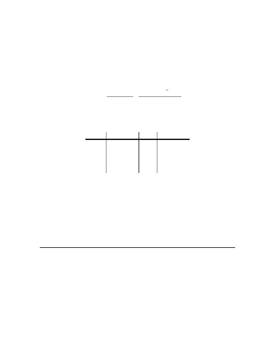
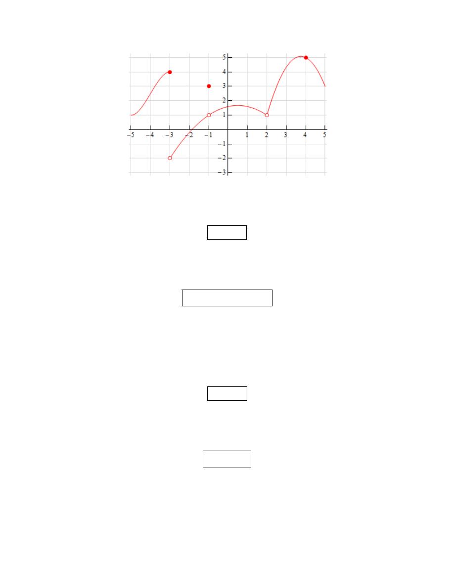
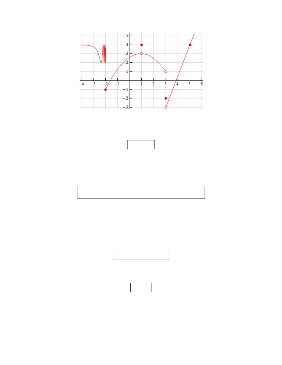
4. Below is the graph of

( )

f x

. For each of the given points determine the value of

( )

f a

and

( )

lim

f x

→

. If any of the quantities do not exist clearly explain why.

(a)

= −

(b)

= −

(c)

(d)

Calculus I

http://tutorial.math.lamar.edu/terms.aspx

(a)

= −

From the graph we can see that,

( )

− =

because the closed dot is at the value of

We can also see that as we approach

= −

from both sides the graph is approaching different

values (4 from the left and -2 from the right). Because of this we get,

( )

lim

does not exist

f x

→−

Always recall that the value of a limit does not actually depend upon the value of the function at
the point in question. The value of a limit only depends on the values of the function around the
point in question. Often the two will be different.

(b)

= −

From the graph we can see that,

( )

− =

because the closed dot is at the value of

We can also see that as we approach

= −

from both sides the graph is approaching the same

value, 1, and so we get,

( )

lim

f x

→−

(c)

Calculus I

http://tutorial.math.lamar.edu/terms.aspx

Because there is no closed dot for

we can see that,

( )

2 does not exist

We can also see that as we approach

from both sides the graph is approaching the same

value, 1, and so we get,

( )

lim

f x

→

(d)

From the graph we can see that,

( )

because the closed dot is at the value of

We can also see that as we approach

from both sides the graph is approaching the same

value, 5, and so we get,

( )

lim

f x

→

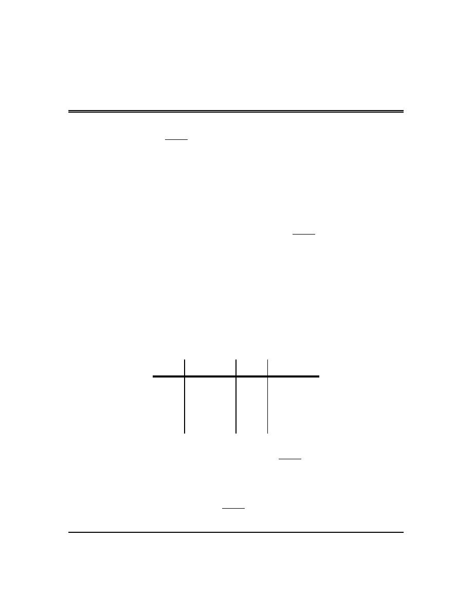
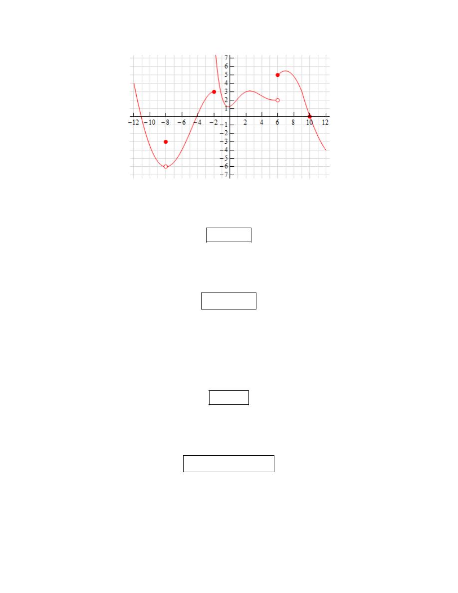
5. Below is the graph of

( )

f x

. For each of the given points determine the value of

( )

f a

and

( )

lim

f x

→

. If any of the quantities do not exist clearly explain why.

(a)

= −

(b)

= −

(c)

(d)

Calculus I

http://tutorial.math.lamar.edu/terms.aspx

(a)

= −

From the graph we can see that,

( )

− = −

because the closed dot is at the value of

= −

We can also see that as we approach

= −

from both sides the graph is approaching the same

value, -6, and so we get,

( )

lim

f x

→−

= −

(b)

= −

From the graph we can see that,

( )

− =

because the closed dot is at the value of

We can also see that as we approach

= −

from both sides the graph is approaching different

values (3 from the left and doesn’t approach any value from the right). Because of this we get,

( )

lim

does not exist

f x

→−

(c)

Calculus I

http://tutorial.math.lamar.edu/terms.aspx

From the graph we can see that,

( )

because the closed dot is at the value of

We can also see that as we approach

from both sides the graph is approaching different

values (2 from the left and 5 from the right). Because of this we get,

( )

lim

does not exist

f x

→

(d)

From the graph we can see that,

( )

because the closed dot is at the value of

We can also see that as we approach

from both sides the graph is approaching the same

value, 0, and so we get,

( )

lim

f x

→

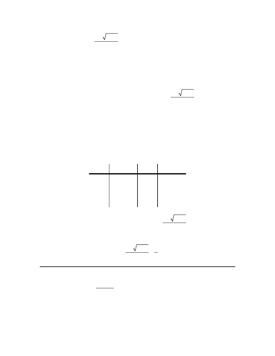
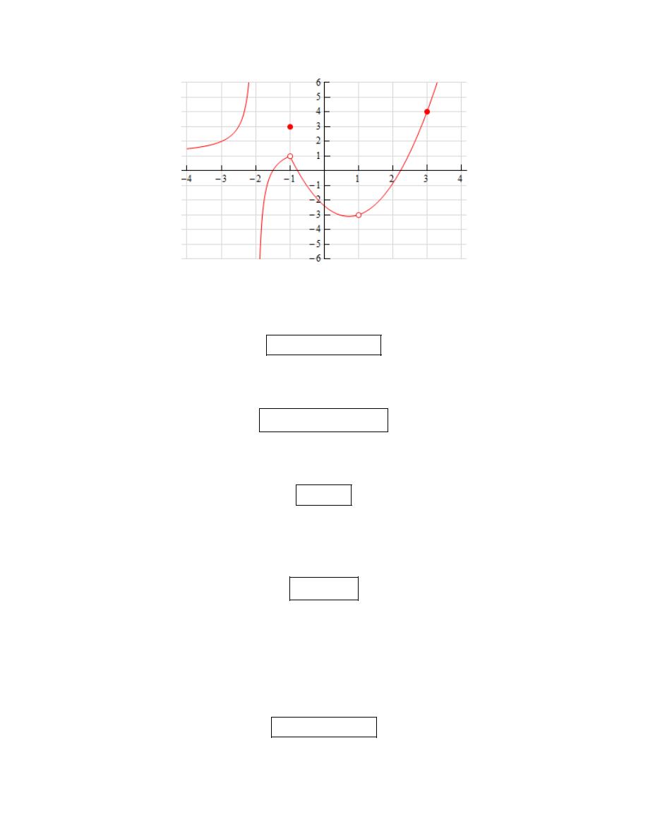
6. Below is the graph of

( )

f x

. For each of the given points determine the value of

( )

f a

and

( )

lim

f x

→

. If any of the quantities do not exist clearly explain why.

(a)

= −

(b)

= −

(c)

(d)

Calculus I

http://tutorial.math.lamar.edu/terms.aspx

(a)

= −

Because there is no closed dot for

= −

we can see that,

( )

2 does not exist

−

We can also see that as we approach

= −

from both sides the graph is not approaching a value

from either side and so we get,

( )

lim

does not exist

f x

→−

(b)

= −

From the graph we can see that,

( )

− =

because the closed dot is at the value of

We can also see that as we approach

= −

from both sides the graph is approaching the same

value, 1, and so we get,

( )

lim

f x

→−

(c)

Because there is no closed dot for

we can see that,

( )

1 does not exist

Calculus I

http://tutorial.math.lamar.edu/terms.aspx

We can also see that as we approach

from both sides the graph is approaching the same

value, -3, and so we get,

( )

lim

f x

→

= −

(d)

From the graph we can see that,

( )

because the closed dot is at the value of

We can also see that as we approach

from both sides the graph is approaching the same

value, 4, and so we get,

( )

lim

f x

→

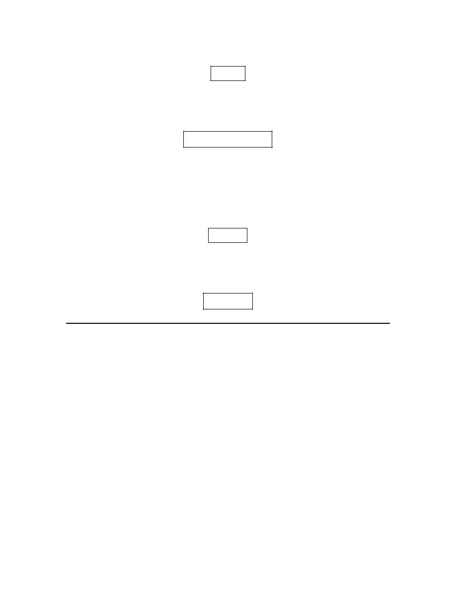
One-Sided Limits

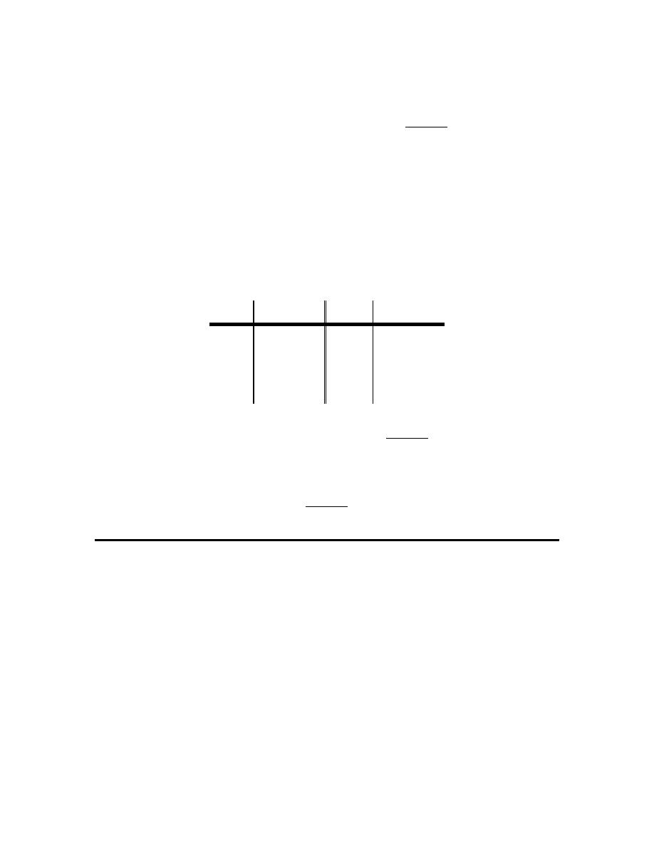
1. Below is the graph of

( )

f x

. For each of the given points determine the value of

( )

f a

( )

lim

f x

−

→

( )

lim

f x

→

, and

( )

lim

f x

→

. If any of the quantities do not exist clearly explain why.

(a)

= −

(b)

= −

(c)

(d)

Calculus I

http://tutorial.math.lamar.edu/terms.aspx

(a)

= −

From the graph we can see that,

( )

− =

because the closed dot is at the value of

We can also see that as we approach

= −

from the left the graph is approaching a value of 3

and as we approach from the right the graph is approaching a value of -2. Therefore we get,

( )

lim

f x

−

→−

= −

Now, because the two one-sided limits are different we know that,

( )

lim

does not exist

f x

→−

(b)

= −

From the graph we can see that,

( )

− =

because the closed dot is at the value of

We can also see that as we approach

= −

from both sides the graph is approaching the same

value, 4, and so we get,

( )

lim

f x

−

→−

The two one-sided limits are the same and so we know,

( )

lim

f x

→−

Calculus I

http://tutorial.math.lamar.edu/terms.aspx

(c)

From the graph we can see that,

( )

= −

because the closed dot is at the value of

= −

We can also see that as we approach

from the left the graph is approaching a value of -1

and as we approach from the right the graph is approaching a value of 5. Therefore we get,

( )

lim

f x

−

→

= −

Now, because the two one-sided limits are different we know that,

( )

lim

does not exist

f x

→

(d)

Because there is no closed dot for

we can see that,

( )

4 does not exist

We can also see that as we approach

from both sides the graph is approaching the same

value, 2, and so we get,

( )

lim

f x

−

→

The two one-sided limits are the same and so we know,

( )

lim

f x

→

Always recall that the value of a limit (including one-sided limits) does not actually depend upon
the value of the function at the point in question. The value of a limit only depends on the values
of the function around the point in question. Therefore, even though the function doesn’t exist at
this point the limit and one-sided limits can still have a value.

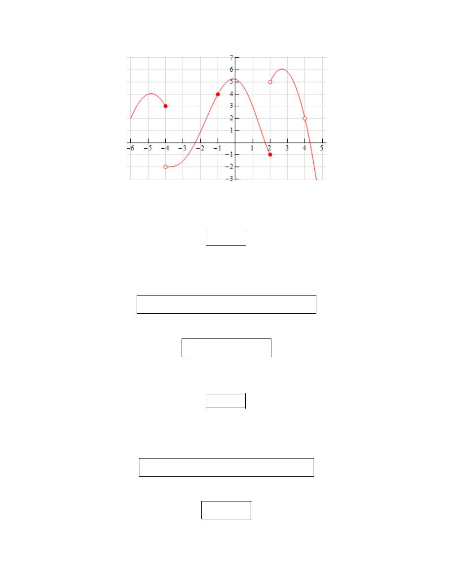
2. Below is the graph of

( )

f x

. For each of the given points determine the value of

( )

f a

( )

lim

f x

−

→

( )

lim

f x

→

, and

( )

lim

f x

→

. If any of the quantities do not exist clearly explain why.

(a)

= −

(b)

(c)

(d)

Calculus I

http://tutorial.math.lamar.edu/terms.aspx

(a)

= −

From the graph we can see that,

( )

− = −

because the closed dot is at the value of

= −

We can also see that as we approach

= −

from the left the graph is not approaching a single

value, but instead oscillating wildly, and as we approach from the right the graph is approaching a
value of -1. Therefore we get,

( )

lim

does not exist

lim

f x

−

→−

= −

Recall that in order for limit to exist the function must be approaching a single value and so, in

this case, because the graph to the left of

= −

is not approaching a single value the left-hand

limit will not exist. This does not mean that the right-hand limit will not exist. In this case the

graph to the right of

= −

is approaching a single value the right-hand limit will exist.

Now, because the two one-sided limits are different we know that,

( )

lim

does not exist

f x

→−

(b)

From the graph we can see that,

( )

because the closed dot is at the value of

We can also see that as we approach

from both sides the graph is approaching the same

value, 3, and so we get,

Calculus I

http://tutorial.math.lamar.edu/terms.aspx

( )

lim

f x

−

→

The two one-sided limits are the same and so we know,

( )

lim

f x

→

(c)

From the graph we can see that,

( )

= −

because the closed dot is at the value of

= −

We can also see that as we approach

from the left the graph is approaching a value of 1

and as we approach from the right the graph is approaching a value of -3. Therefore we get,

( )

lim

f x

−

→

= −

Now, because the two one-sided limits are different we know that,

( )

lim

does not exist

f x

→

(d)

From the graph we can see that,

( )

because the closed dot is at the value of

We can also see that as we approach

from both sides the graph is approaching the same

value, 4, and so we get,

( )

lim

f x

−

→

The two one-sided limits are the same and so we know,

( )

lim

f x

→

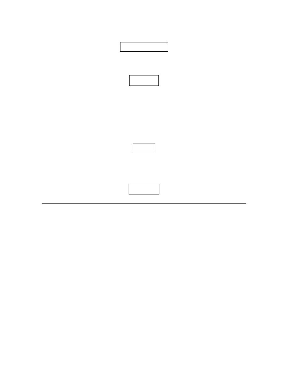
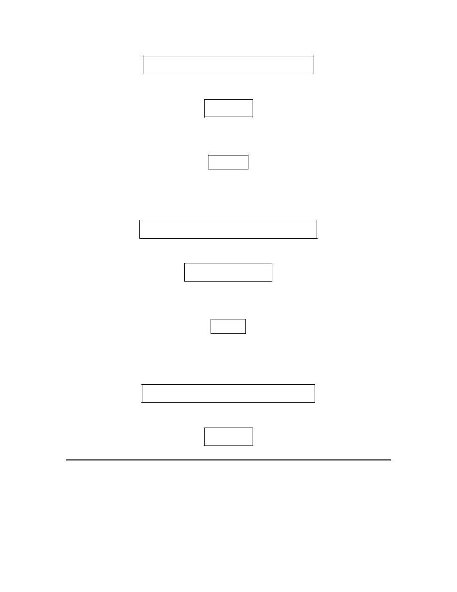
3. Sketch a graph of a function that satisfies each of the following conditions.

( )

lim

f x

−

→

= −

Solution

Calculus I

http://tutorial.math.lamar.edu/terms.aspx

There are literally an infinite number of possible graphs that we could give here for an answer.

However, all of them must have a closed dot on the graph at the point

( )

2,1

, the graph must be

approaching a value of 1 as it approaches

from the left (as indicated by the left-hand limit)

and it must be approaching a value of -4 as it approaches

from the right (as indicated by

the right-hand limit).

Here is a sketch of one possible graph that meets these conditions.

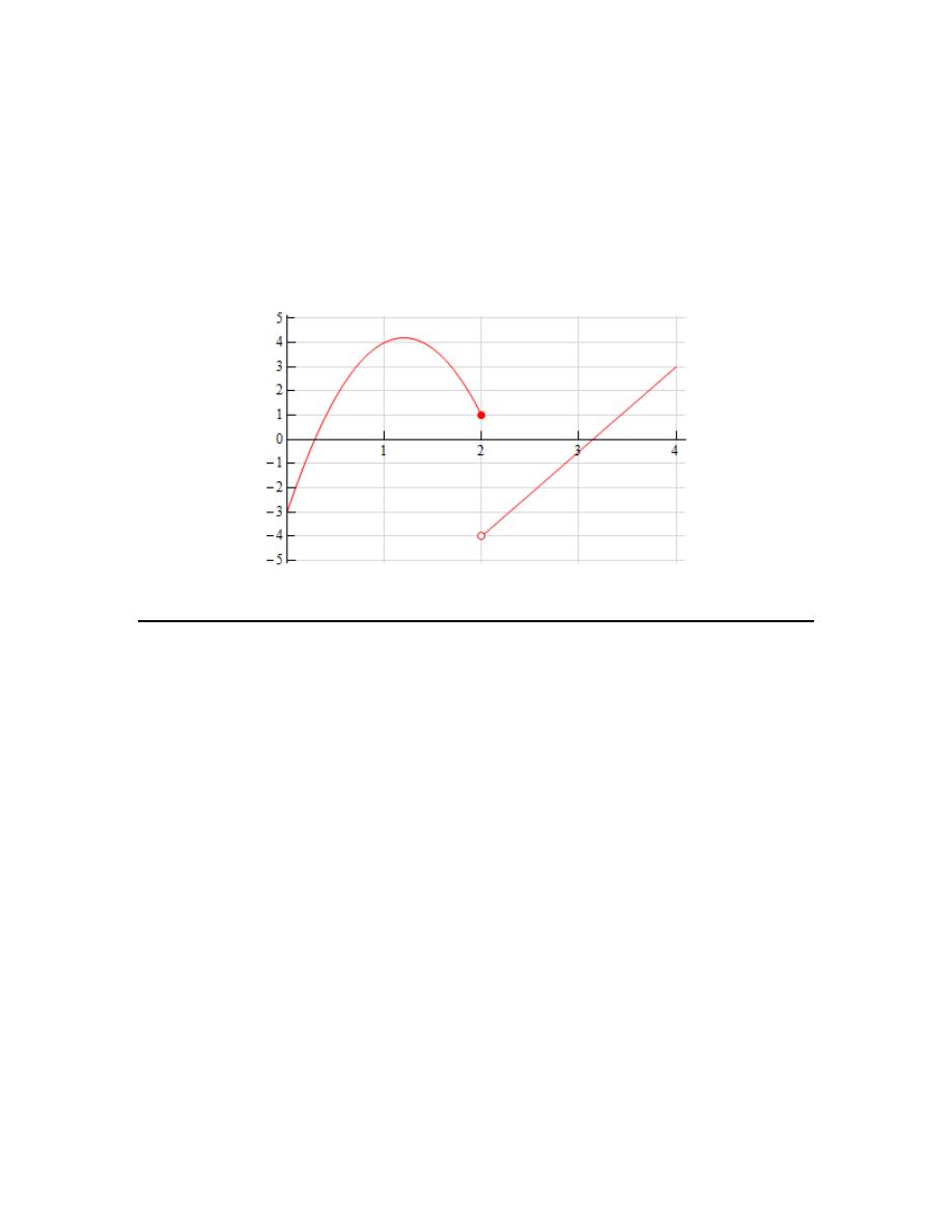
4. Sketch a graph of a function that satisfies each of the following conditions.

( )

lim

3 does not exist

lim

f x

−

→

→−

= −

− =

Solution
There are literally an infinite number of possible graphs that we could give here for an answer.
However, all of them must the following two sets of criteria.

First, at

there cannot be a closed dot on the graph (as indicated by the fact that the function

does not exist here), the graph must be approaching a value of 0 as it approaches

from the

left (as indicated by the left-hand limit) and it must be approaching a value of 4 as it approaches

from the right (as indicated by the right-hand limit).

Next, the graph must have a closed dot at the point

(

)

1, 2

−

and the graph must be approaching a

value of -3 as it approaches

= −

from both sides (as indicated by the fact that value of the

overall limit is -3 at this point).

Here is a sketch of one possible graph that meets these conditions.

Calculus I

http://tutorial.math.lamar.edu/terms.aspx

Calculus I

http://tutorial.math.lamar.edu/terms.aspx

Limit Properties

1. Given

( )

lim

f x

→

= −

( )

lim

g x

→

and

( )

lim

h x

→

use the limit properties given in this

section to compute each of the following limits. If it is not possible to compute any of the limits
clearly explain why not.

(a)

( )

lim 2

f x

h x

→

−









(b)

( )

lim 3

h x

→

−









(c)

( ) ( )

( )

lim

g x h x

f x

→

−









(d)

( ) ( ) ( )

lim

f x

g x

h x

→

−









Hint : For each of these all we need to do is use the limit properties on the limit until the given
limits appear and we can then compute the value.

(a)

( )

lim 2

f x

h x

→

−









Here is the work for this limit. At each step the property (or properties) used are listed and note
that in some cases the properties may have been used more than once in the indicated step.

( )

lim 2

lim 12

Property 2

2 lim

12 lim

Property 1

12 4

Plug in values of limits

f x

h x

f x

h x

f x

h x

→

−

























−

− −

= −

(b)

( )

lim 3

h x

→

−









Here is the work for this limit. At each step the property (or properties) used are listed and note
that in some cases the properties may have been used more than once in the indicated step.

( )

lim 3

lim 6

Property 2

3lim

lim 6

Property 1

3 4

Plug in value of limits & Property 7

h x

→

−

















−

(c)

( ) ( )

( )

lim

g x h x

f x

→

−









Calculus I

http://tutorial.math.lamar.edu/terms.aspx

Here is the work for this limit. At each step the property (or properties) used are listed and note
that in some cases the properties may have been used more than once in the indicated step.

( ) ( )

( )

( ) ( )

( )

( )( ) ( )

lim

Property 2

lim

Property 3

2 4

Plug in values of limits

g x h x

f x

g x h x

f x

g x

h x

f x

→

−



















 



−



 



− −

(d)

( ) ( ) ( )

lim

f x

g x

h x

→

−









Here is the work for this limit. At each step the property (or properties) used are listed and note
that in some cases the properties may have been used more than once in the indicated step.

( ) ( ) ( )

( )

lim

Property 2

9 2 4

Plug in values of limits

f x

g x

h x

f x

g x

h x

→

−









= − − +
= −

2. Given

( )

lim

f x

→−

( )

lim

g x

→−

and

( )

lim

h x

→−

= −

use the limit properties given in

this section to compute each of the following limits. If it is not possible to compute any of the
limits clearly explain why not.

(a)

( )

lim

f x

h x

g x

f x

→−





−









(b)

( ) ( ) ( )

lim

f x g x h x

→−









(c)

( )

( ) ( )

lim

f x

h x

g x

h x

→−





−









(d)

( ) ( ) ( )

lim 2

h x

f x

→−





−









Hint : For each of these all we need to do is use the limit properties on the limit until the given
limits appear and we can then compute the value.

(a)

( )

lim

f x

h x

g x

f x

→−





−









Here is the work for this limit. At each step the property (or properties) used are listed and note
that in some cases the properties may have been used more than once in the indicated step.

Calculus I

http://tutorial.math.lamar.edu/terms.aspx

( )

lim

Property 2

lim

Property 4

lim

Plug in values of limits

f x

h x

f x

h x

g x

f x

g x

f x

h x

g x

f x

→−





−









−

Note that were able to use Property 4 in the second step only because after we evaluated the limit
of the denominators (both of them) we found that the limits of the denominators were not zero.

(b)

( ) ( ) ( )

lim

f x g x h x

→−









Here is the work for this limit. At each step the property (or properties) used are listed and note
that in some cases the properties may have been used more than once in the indicated step.

( ) ( ) ( )

( )

( )( )( )

lim

Property 3

1 10

Plug in value of limits

f x g x h x

f x

g x

h x

→−



 









 



−

= −

Note that the properties 2 & 3 in this section were only given with two functions but they can
easily be extended out to more than two functions as we did here for property 3.

(c)

( )

( ) ( )

lim

f x

h x

g x

h x

→−





−









Here is the work for this limit. At each step the property (or properties) used are listed and note
that in some cases the properties may have been used more than once in the indicated step.

Calculus I

http://tutorial.math.lamar.edu/terms.aspx

( )

( ) ( )

( )

( ) ( )

( )

( ) ( )

( )

lim

Property 2

lim 1

lim 3

Property 4

lim

lim 1

lim 3

lim

Property 2

lim

3 1

f x

h x

g x

h x

g x

h x

f x

h x

g x

h x

f x

h x

g x

h x

→−





−









−

















−

Plug in values of limits

& Property 1

−

Note that were able to use Property 4 in the second step only because after we evaluated the limit
of the denominators (both of them) we found that the limits of the denominators were not zero.

(d)

( ) ( ) ( )

lim 2

h x

f x

→−





−









Here is the work for this limit. At each step the property (or properties) used are listed and note
that in some cases the properties may have been used more than once in the indicated step.

( ) ( ) ( )

( )

lim 2

lim

Property 2

lim 1

lim 2

Property 4

lim

h x

f x

h x

f x

h x

f x

→−





−









−









At this point let’s step back a minute. In the previous parts we didn’t worry about using property
4 on a rational expression. However, in this case let’s be a little more careful. We can only use
property 4 if the limit of the denominator is not zero. Let’s check that limit and see what we get.

( )

lim

lim 7

Property 2

lim

7 lim

Property 1

7 7 1

Plug in values of limits & Property 1

h x

f x

h x

f x

h x

f x

→−

















= − +
=

Okay, we can see that the limit of the denominator in the second term will be zero and so we can
not actually use property 4 on that term. This means that this limit cannot be done and note that

Calculus I

http://tutorial.math.lamar.edu/terms.aspx

the fact that we could determine a value for the limit of the first term will not change this fact.
This limit cannot be done.

3. Given

( )

lim

f x

→

( )

lim

g x

→

= −

and

( )

lim

h x

→

= −

use the limit properties given in this

section to compute each of the following limits. If it is not possible to compute any of the limits
clearly explain why not.

(a)

( ) ( )

lim

f x

h x

→









(b)

( ) ( )

lim

g x h x

→

(c)

( )

lim 11

g x

→

+ 







(d)

( )

( ) ( )

lim

f x

h x

g x

→

−

Hint : For each of these all we need to do is use the limit properties on the limit until the given
limits appear and we can then compute the value.

(a)

( ) ( )

lim

f x

h x

→









Here is the work for this limit. At each step the property (or properties) used are listed and note
that in some cases the properties may have been used more than once in the indicated step.

( ) ( )

(

)

( )

[

]

lim

Property 5

lim

Property 2

6 1

Plug in values of limits

125

f x

h x

f x

h x

f x

h x

→

























= −
=

(b)

( ) ( )

lim

g x h x

→

Here is the work for this limit. At each step the property (or properties) used are listed and note
that in some cases the properties may have been used more than once in the indicated step.

( ) ( )

( )

( )( )

lim

Property 6

lim

Property 3

Plug in value of limits

g x h x

g x

h x

→



 



= 

 



−

Calculus I

http://tutorial.math.lamar.edu/terms.aspx

(c)

( )

lim 11

g x

→

+ 







Here is the work for this limit. At each step the property (or properties) used are listed and note
that in some cases the properties may have been used more than once in the indicated step.

( )

(

)

( )

lim 11

Property 6

lim11 lim

Property 2

lim11

lim

Property 5

Plug in values of limits & Property 7

g x

→





























+ 



+ −

(d)

( )

lim

f x

h x

g x

→

−

Here is the work for this limit. At each step the property (or properties) used are listed and note
that in some cases the properties may have been used more than once in the indicated step.

( )

( ) ( )

( )

( ) ( )

( )

( ) ( )

(

)

( )

lim

Property 6

lim

Property 4

lim

Property 2

lim

Plug in values of limits

f x

h x

g x

h x

g x

f x

h x

g x

f x

h x

g x

→

−

− − −

Note that were able to use Property 4 in the second step only because after we evaluated the limit
of the denominators (both of them) we found that the limits of the denominators were not zero.

4. Use the limit properties given in this section to compute the following limit. At each step
clearly indicate the property being used. If it is not possible to compute any of the limits clearly
explain why not.

Calculus I

http://tutorial.math.lamar.edu/terms.aspx

(

)

lim 14 6

→−

− +

Hint : All we need to do is use the limit properties on the limit until we can use Properties 7, 8
and/or 9 from this section to compute the limit.

(

)

( ) ( )

lim 14 6

lim 14

lim 6

lim

Property 2

lim 14 6 lim

lim

Property 1

14 6

Properties 7, 8, & 9

→−

− +

−

− − + −

5. Use the limit properties given in this section to compute the following limit. At each step
clearly indicate the property being used. If it is not possible to compute any of the limits clearly
explain why not.

(

)

lim 3

→

−

Hint : All we need to do is use the limit properties on the limit until we can use Properties 7, 8
and/or 9 from this section to compute the limit.

(

)

( )

lim 3

lim 7

lim16

Property 2

3lim

7 lim

lim16

Property 1

3 6

7 6

Properties 7, 8, & 9

134

→

−

6. Use the limit properties given in this section to compute the following limit. At each step
clearly indicate the property being used. If it is not possible to compute any of the limits clearly
explain why not.

lim

4 7

→

−

Hint : All we need to do is use the limit properties on the limit until we can use Properties 7, 8
and/or 9 from this section to compute the limit.

Calculus I

http://tutorial.math.lamar.edu/terms.aspx

(

)

(

)

( )

lim

Property 4

4 7

lim 4 7

lim

lim 8

Property 2

lim 4 lim 7

lim

8 lim

Property 1

lim 4 7 lim

8 3

Properties 7, 8, & 9

4 7 3

→

−

Note that we were able to use property 4 in the first step because after evaluating the limit in the
denominator we found that it wasn’t zero.

7. Use the limit properties given in this section to compute the following limit. At each step
clearly indicate the property being used. If it is not possible to compute any of the limits clearly
explain why not.

lim

→−

−

Hint : All we need to do is use the limit properties on the limit until we can use Properties 7, 8
and/or 9 from this section to compute the limit.

(

)

(

)

lim

Property 4

lim

→−

−

Okay, at this point let’s step back a minute. We used property 4 here and we know that we can
only do that if the limit of the denominator is not zero. So, let’s check that out and see what we
get.

(

)

( )

lim

lim 3

lim 10

Property 2

lim

3 lim

lim 10

Property 1

Properties 7, 8, & 9

→−

−

= −

+ − −

Calculus I

http://tutorial.math.lamar.edu/terms.aspx

So, the limit of the denominator is zero and so we couldn’t use property 4 in this case. Therefore,
we cannot do this limit at this point (note that it will be possible to do this limit after the next
section).

8. Use the limit properties given in this section to compute the following limit. At each step
clearly indicate the property being used. If it is not possible to compute any of the limits clearly
explain why not.

lim

→

Hint : All we need to do is use the limit properties on the limit until we can use Properties 7, 8
and/or 9 from this section to compute the limit.

(

)

lim

Property 6

lim

lim 6

Property 2

Properties 7 & 9

→

+ =

9. Use the limit properties given in this section to compute the following limit. At each step
clearly indicate the property being used. If it is not possible to compute any of the limits clearly
explain why not.

(

)

lim 4

→

−

Hint : All we need to do is use the limit properties on the limit until we can use Properties 7, 8
and/or 9 from this section to compute the limite.

(

)

(

)

( )

lim 4

lim

Property 2

lim 4

lim

Property 6

lim 4

lim

lim 2

Property 2

4 lim

lim

lim 2

Property 1

4 10

10 2

Properties 7 & 8

→

−

Calculus I

http://tutorial.math.lamar.edu/terms.aspx

Computing Limits

1. Evaluate

(

)

lim 8 3

→

−

, if it exists.

Solution
There is not really a lot to this problem. Simply recall the basic ideas for computing limits that
we looked at in this section. We know that the first thing that we should try to do is simply plug
in the value and see if we can compute the limit.

(

)

( )

lim 8 3

8 3 2

12 4

→

−

= −

2. Evaluate

6 4

lim

→−

, if it exists.

lim

→−

−

= −

3. Evaluate

lim

→−

−

, if it exists.

Solution
There is not really a lot to this problem. Simply recall the basic ideas for computing limits that
we looked at in this section. In this case we see that if we plug in the value we get 0/0. Recall
that this DOES NOT mean that the limit doesn’t exist. We’ll need to do some more work before
we make that conclusion. All we need to do here is some simplification and then we’ll reach a
point where we can plug in the value.

Calculus I

http://tutorial.math.lamar.edu/terms.aspx

(

)(

)

(

)(

)

lim

→−

−

4. Evaluate

lim

→

−

, if it exists.

(

)(

)

(

)

lim

→

−

= −

−

− −

−

5. Evaluate

lim

→

−

, if it exists.

(

)(

)

(

)(

)

lim

→

−

6. Evaluate

(

)

lim

→

−

, if it exists.

Calculus I

http://tutorial.math.lamar.edu/terms.aspx

we make that conclusion. All we need to do here is some simplification and then we’ll reach a
point where we can plug in the value.

(

)

(

)

(

)

36 12

lim

lim 12

→

−

7. Evaluate

lim

→

−

, if it exists.

Solution
There is not really a lot to this problem. Simply recall the basic ideas for computing limits that
we looked at in this section. In this case we see that if we plug in the value we get 0/0. Recall
that this DOES NOT mean that the limit doesn’t exist. We’ll need to do some more work before
we make that conclusion. If you’re really good at factoring you can factor this and simplify.
Another method that can be used however is to rationalize the numerator, so let’s do that for this
problem.

(

)

(

)

(

)

(

)

(

)

(

)

lim

→

−

8. Evaluate

lim

→−

−

, if it exists.

Solution
There is not really a lot to this problem. Simply recall the basic ideas for computing limits that
we looked at in this section. In this case we see that if we plug in the value we get 0/0. Recall
that this DOES NOT mean that the limit doesn’t exist. We’ll need to do some more work before
we make that conclusion. Simply factoring will not do us much good here so in this case it looks
like we’ll need to rationalize the numerator.

(

)

(

)

(

)

(

)

(

)

(

)

(

)

(

)

(

)

22 16

lim

→−

−

= =

Calculus I

http://tutorial.math.lamar.edu/terms.aspx

9. Evaluate

lim

→

−

, if it exists.

Solution
There is not really a lot to this problem. Simply recall the basic ideas for computing limits that
we looked at in this section. In this case we see that if we plug in the value we get 0/0. Recall
that this DOES NOT mean that the limit doesn’t exist. We’ll need to do some more work before
we make that conclusion. Simply factoring will not do us much good here so in this case it looks
like we’ll need to rationalize the denominator.

(

)

(

)

(

)

(

)

(

)

(

)

lim

→

− +

−

= −

−

10. Given the function

( )

7 4

f x

−



= 

≥



Evaluate the following limits, if they exist.

(a)

( )

lim

f x

→−

(b)

( )

lim

f x

→

Hint : Recall that when looking at overall limits (as opposed to one-sided limits) we need to make
sure that the value of the function must be approaching the same value from both sides. In other
words, the two one sided limits must both exist and be equal.

(a)

( )

lim

f x

→−

Solution

For this part we know that

6 1

− <

and so there will be values of x on both sides of -6 in the range

and so we can assume that, in the limit, we will have

. This will allow us to use the

piece of the function in that range and then just use standard limit techniques to compute the
limit.

( )

(

)

lim

lim 7 4

f x

→−

−

(b)

( )

lim

f x

→

Solution

This part is going to be different from the previous part. We are looking at the limit at

and

that is the “cut–off” point in the piecewise functions. Recall from the discussion in the section,
that this means that we are going to have to look at the two one sided limits.

Calculus I

http://tutorial.math.lamar.edu/terms.aspx

( )

(

)

lim

lim 7 4

because

1 implies that

f x

−

→

−

→

( )

(

)

lim

because

1 implies that

f x

→

So, in this case, we can see that,

( )

lim

f x

−

→

and so we know that the overall limit must exist and,

( )

lim

f x

→

11. Given the function

( )

1 9

h z

≤ −



= 

−

> −



Evaluate the following limits, if they exist.

(a)

( )

lim

h z

→

(b)

( )

lim

h z

→−

(a)

( )

lim

h z

→

Solution

For this part we know that

> −

and so there will be values of z on both sides of 7 in the range

> −

and so we can assume that, in the limit, we will have

> −

. This will allow us to use

the piece of the function in that range and then just use standard limit techniques to compute the
limit.

( )

(

)

lim

lim 1 9

h z

→

−

= −

(b)

( )

lim

h z

→−

Solution

This part is going to be different from the previous part. We are looking at the limit at

= −

and that is the “cut–off” point in the piecewise functions. Recall from the discussion in the
section, that this means that we are going to have to look at the two one sided limits.

( )

lim

lim 6

because

4 implies that

h z

−

→−

= −

→ −

< −

( )

(

)

lim

lim 1 9

because

4 implies that

h z

→−

−

→ −

> −

Calculus I

http://tutorial.math.lamar.edu/terms.aspx

So, in this case, we can see that,

( )

lim

h z

−

→−

= − ≠

and so we know that the overall limit does not exist.

12. Evaluate

(

)

lim 10

→

+ −

, if it exists.

Hint : Recall the mathematical definition of the absolute value function and that it is in fact a
piecewise function.

Solution
Recall the definition of the absolute value function.

≥



= 

−



So, because the function inside the absolute value is zero at

we can see that,

(

)

−

≥



− = 

− −



This means that we are being asked to compute the limit at the “cut–off” point in a piecewise
function and so, as we saw in this section, we’ll need to look at two one-sided limits in order to
determine if this limit exists (and its value if it does exist).

(

)

(

)

(

)

(

)

lim 10

lim 15

recall

5 implies

−

→

+ −

− −

−

→

(

)

(

)

(

)

(

)

lim 10

lim 5

recall

5 implies

−

→

+ −

−

→

So, for this problem, we can see that,

(

)

(

)

lim 10

−

→ +

→

+ −

and so the overall limit must exist and,

(

)

lim 10

−

→

+ −

13. Evaluate

lim

→−

+
+

, if it exists.

Hint : Recall the mathematical definition of the absolute value function and that it is in fact a
piecewise function.

Calculus I

http://tutorial.math.lamar.edu/terms.aspx

Solution
Recall the definition of the absolute value function.

≥



= 

−



So, because the function inside the absolute value is zero at

= −

we can see that,

(

)

≥ −



+ = 

− +

< −



(

)

lim

lim 1

recall

1 implies

−

→−

− = −

→ −

< −

− +

lim

lim 1 1

recall

1 implies

→−

→ −

> −

So, for this problem, we can see that,

lim

1 1

lim

−

→−

= − ≠ =

and so the overall limit does not exist.

14. Given that

( )

f x

≤

for all x determine the value of

( )

lim

f x

→

Hint : Recall the Squeeze Theorem.

Solution

This problem is set up to use the Squeeze Theorem. First, we already know that

( )

f x

is always

between two other functions. Now all that we need to do is verify that the two “outer” functions

have the same limit at

and if they do we can use the Squeeze Theorem to get the answer.

(

)

lim 7

lim 3

→

So, we have,

(

)

lim 7

lim 3

→

and so by the Squeeze Theorem we must also have,

Calculus I

http://tutorial.math.lamar.edu/terms.aspx

( )

lim

f x

→

15. Use the Squeeze Theorem to determine the value of

lim

sin

→

 

 

 

Hint : Recall how we worked the Squeeze Theorem problem in this section to find the lower and
upper functions we need in order to use the Squeeze Theorem.

Solution
We first need to determine lower/upper functions. We’ll start off by acknowledging that

provided

≠

(which we know it won’t be because we are looking at the limit as

→

) we

will have,

1 sin

 

− ≤

≤

 

 

Now, simply multiply through this by

to get,

sin

 

− ≤

≤

 

 

Before proceeding note that we can only do this because we know that

for

≠

. Recall

that if we multiply through an inequality by a negative number we would have had to switch the

signs. So, for instance, had we multiplied through by

we would have had issues because this

is positive if

and negative if

Now, let’s get back to the problem. We have a set of lower/upper functions and clearly,

( )

lim

→

−

Therefore, by the Squeeze Theorem we must have,

lim

sin

→

  =

 

 

Infinite Limits

Calculus I

http://tutorial.math.lamar.edu/terms.aspx

1. For

( )

(

)

f x

−

evaluate the indicated limits, if they exist.

(a)

( )

lim

f x

−

→

(b)

( )

lim

f x

→

(c)

( )

lim

f x

→

(a)

( )

lim

f x

−

→

Let’s start off by acknowledging that for

−

→

we know

For the numerator we can see that, in the limit, it will just be 9.

The denominator takes a little more work. Clearly, in the limit, we have,

− →

but we can actually go a little farther. Because we know that

we also know that,

− <

More compactly, we can say that in the limit we will have,

−

− →

Raising this to the fifth power will not change this behavior and so, in the limit, the denominator
will be,

(

)

−

→

We can now do the limit of the function. In the limit, the numerator is a fixed positive constant
and the denominator is an increasingly small negative number. In the limit, the quotient must
then be an increasing large negative number or,

(

)

lim

−

→

= −∞

−

Note that this also means that there is a vertical asymptote at

(b)

( )

lim

f x

→

Let’s start off by acknowledging that for

→

we know

As in the first part the numerator, in the limit, it will just be 9.

The denominator will also work similarly to the first part. In the limit, we have,

− →

and because we know that

we also know that,

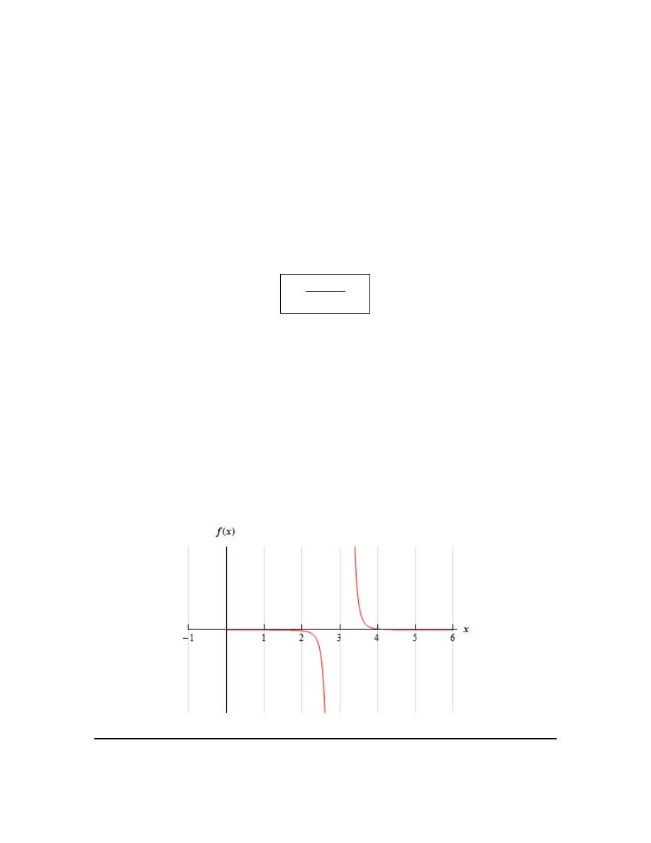
Calculus I

http://tutorial.math.lamar.edu/terms.aspx

− >

More compactly, we can say that in the limit we will have,

− →

Raising this to the fifth power will not change this behavior and so, in the limit, the denominator
will be,

(

)

−

→

We can now do the limit of the function. In the limit, the numerator is a fixed positive constant
and the denominator is an increasingly small positive number. In the limit, the quotient must then
be an increasing large positive number or,

(

)

lim

→

= ∞

−

Note that this also means that there is a vertical asymptote at

, which we already knew from

the first part.

(c)

( )

lim

f x

→

In this case we can see from the first two parts that,

( )

lim

f x

−

→

≠

and so, from our basic limit properties we can see that

( )

lim

f x

→

does not exist.

For the sake of completeness and to verify the answers for this problem here is a quick sketch of
the function.

Calculus I

http://tutorial.math.lamar.edu/terms.aspx

2. For

( )

h t

evaluate the indicated limits, if they exist.

(a)

( )

lim

h t

−

→−

(b)

( )

lim

h t

→−

(c)

( )

lim

h t

→−

(a)

( )

lim

h t

−

→−

Let’s start off by acknowledging that for

−

→ −

we know

< −

For the numerator we can see that, in the limit, we will get -12.

The denominator takes a little more work. Clearly, in the limit, we have,

+ →

but we can actually go a little farther. Because we know that

< −

we also know that,

+ <

More compactly, we can say that in the limit we will have,

−

+ →

So, in the limit, the numerator is approaching a negative number and the denominator is an
increasingly small negative number. The quotient must then be an increasing large positive
number or,

lim

−

→−

= ∞

Note that this also means that there is a vertical asymptote at

= −

(b)

( )

lim

h t

→−

Let’s start off by acknowledging that for

→ −

we know

> −

For the numerator we can see that, in the limit, we will get -12.

The denominator will also work similarly to the first part. In the limit, we have,

+ →

but we can actually go a little farther. Because we know that

> −

we also know that,

+ >

More compactly, we can say that in the limit we will have,

+ →

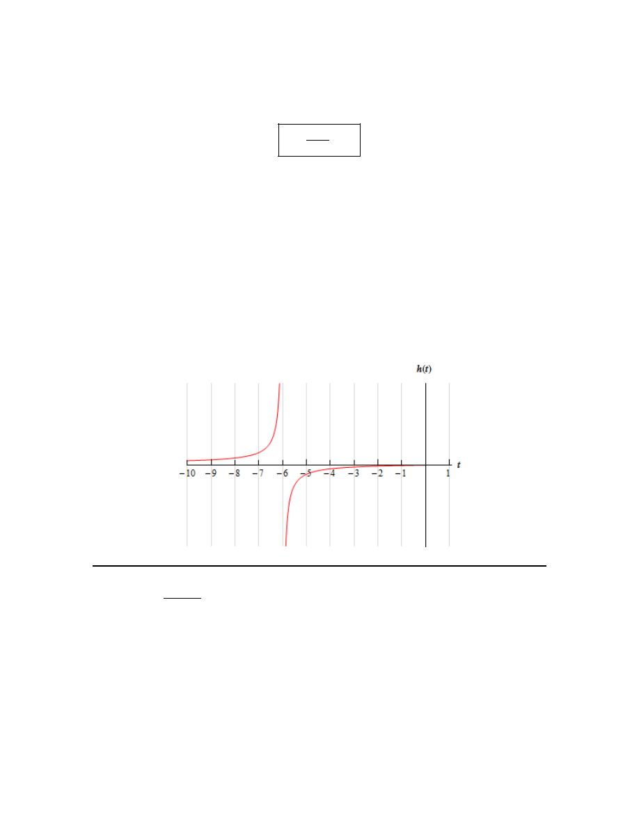
Calculus I

http://tutorial.math.lamar.edu/terms.aspx

So, in the limit, the numerator is approaching a negative number and the denominator is an
increasingly small positive number. The quotient must then be an increasing large negative
number or,

lim

→−

= −∞

Note that this also means that there is a vertical asymptote at

= −

, which we already knew

from the first part.

(c)

( )

lim

h t

→−

In this case we can see from the first two parts that,

( )

lim

h t

−

→−

≠

and so, from our basic limit properties we can see that

( )

lim

h t

→−

does not exist.

For the sake of completeness and to verify the answers for this problem here is a quick sketch of
the function.

3. For

( )

(

)

g z

evaluate the indicated limits, if they exist.

(a)

( )

lim

g z

−

→−

(b)

( )

lim

g z

→−

(c)

( )

lim

g z

→−

(a)

( )

lim

g z

−

→−

Let’s start off by acknowledging that for

−

→ −

we know

< −

Calculus I

http://tutorial.math.lamar.edu/terms.aspx

For the numerator we can see that, in the limit, we will get 2.

Now let’s take care of the denominator. In the limit, we will have,

−

+ →

and upon squaring the

we see that, in the limit, we will have,

(

)

→

So, in the limit, the numerator is approaching a positive number and the denominator is an
increasingly small positive number. The quotient must then be an increasing large positive
number or,

(

)

lim

−

→−

= ∞

Note that this also means that there is a vertical asymptote at

= −

(b)

( )

lim

g z

→−

Let’s start off by acknowledging that for

→ −

we know

For the numerator we can see that, in the limit, we will get 2.

Now let’s take care of the denominator. In the limit, we will have,

+ →

and upon squaring the

we see that, in the limit, we will have,

(

)

→

So, in the limit, the numerator is approaching a positive number and the denominator is an
increasingly small positive number. The quotient must then be an increasing large positive
number or,

(

)

lim

→−

= ∞

Note that this also means that there is a vertical asymptote at

= −

, which we already knew

from the first part.

(c)

( )

lim

g z

→−

In this case we can see from the first two parts that,

( )

lim

g z

−

→−

= ∞

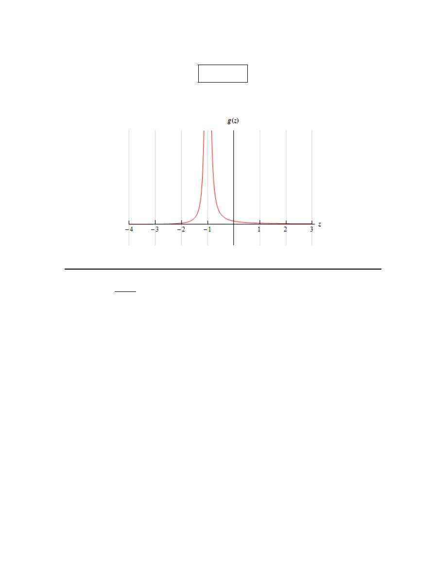
Calculus I

http://tutorial.math.lamar.edu/terms.aspx

and so, from our basic limit properties we can see that,

( )

lim

g z

→−

= ∞

For the sake of completeness and to verify the answers for this problem here is a quick sketch of
the function.

4. For

( )

g x

−

evaluate the indicated limits, if they exist.

(a)

( )

lim

g x

−

→

(b)

( )

lim

g x

→

(c)

( )

lim

g x

→

(a)

( )

lim

g x

−

→

Let’s start off by acknowledging that for

−

→

we know

For the numerator we can see that, in the limit, we will get 9.

Now let’s take care of the denominator. First, we know that if we square a number less than 2
(and greater than -2, which it is safe to assume we have here because we’re doing the limit) we
will get a number that is less that 4 and so, in the limit, we will have,

−

− →

So, in the limit, the numerator is approaching a positive number and the denominator is an
increasingly small negative number. The quotient must then be an increasing large negative
number or,

Calculus I

http://tutorial.math.lamar.edu/terms.aspx

lim

−

→

= −∞

−

Note that this also means that there is a vertical asymptote at

(b)

( )

lim

g x

→

Let’s start off by acknowledging that for

→

we know

For the numerator we can see that, in the limit, we will get 9.

Now let’s take care of the denominator. First, we know that if we square a number greater than 2
we will get a number that is greater than 4 and so, in the limit, we will have,

− →

So, in the limit, the numerator is approaching a positive number and the denominator is an
increasingly small positive number. The quotient must then be an increasing large positive
number or,

lim

→

= ∞

−

Note that this also means that there is a vertical asymptote at

, which we already knew from

the first part.

(c)

( )

lim

g x

→

In this case we can see from the first two parts that,

( )

lim

g x

−

→

≠

and so, from our basic limit properties we can see that

( )

lim

g x

→

does not exist.

For the sake of completeness and to verify the answers for this problem here is a quick sketch of
the function.

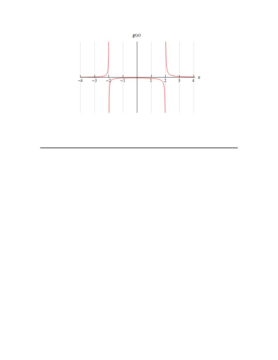
Calculus I

http://tutorial.math.lamar.edu/terms.aspx

As we’re sure that you had already noticed there would be another vertical asymptote at

= −

for this function. For the practice you might want to make sure that you can also do the limits for
that point.

5. For

( )

h x

−

evaluate the indicated limits, if they exist.

(a)

( )

lim

h x

−

→

(b)

( )

lim

h x

→

(c)

( )

lim

h x

→

Hint : Do not get excited about the

−

inside the logarithm. Just recall what you know about

natural logarithms, where they exist and don’t exist and the limits of the natural logarithm at

(a)

( )

lim

h x

−

→

Okay, let’s start off by acknowledging that for

−

→

we know

and so

− >

or,

− →

What this means for us is that this limit does make sense! We know that we can’t have negative
arguments in a logarithm, but because of the negative sign in this particular logarithm that means
that we can use negative x’s in this function (positive x’s on the other hand will now cause
problems of course…).

By Example 6 in the notes for this section we know that as the argument of a logarithm
approaches zero from the right (as ours does in this limit) then the logarithm will approach

−∞

Therefore, the answer for this part is,

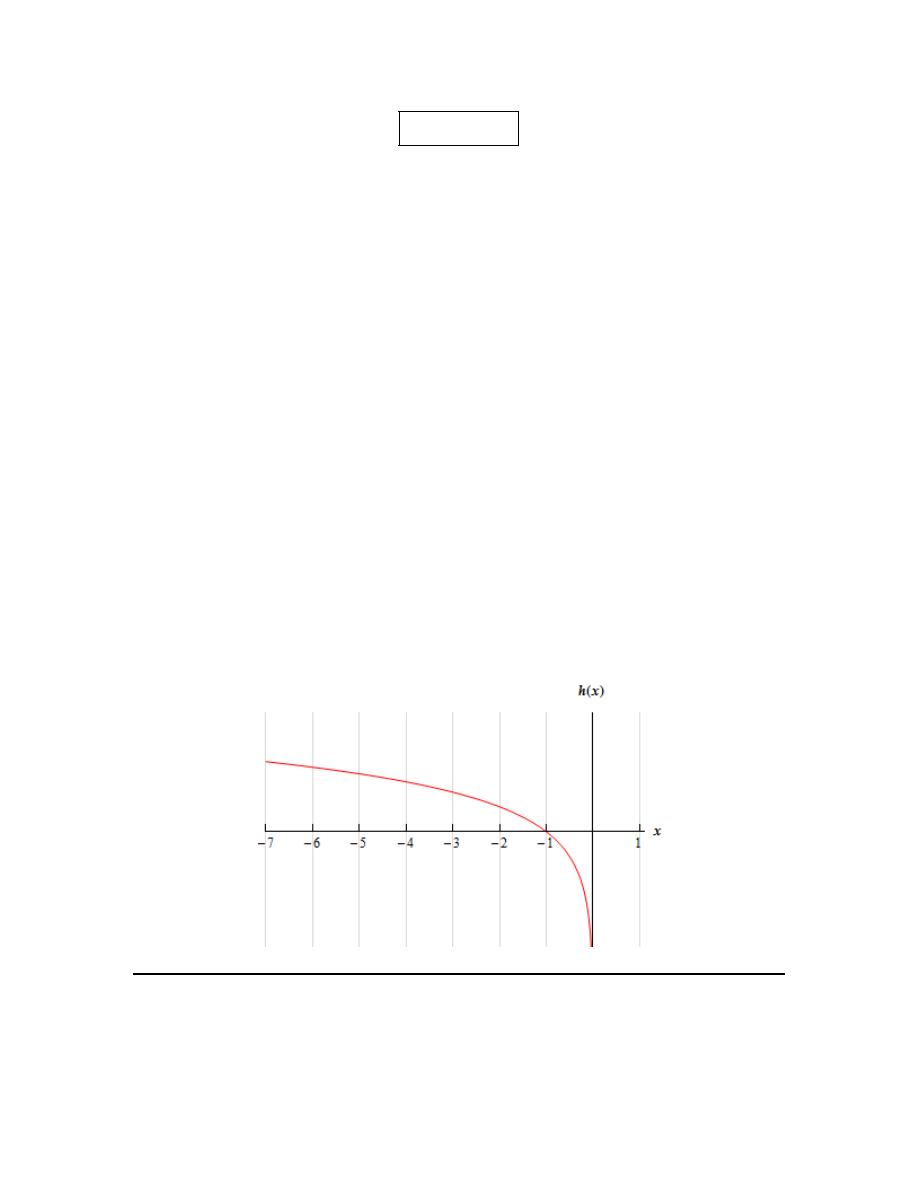
Calculus I

http://tutorial.math.lamar.edu/terms.aspx

( )

lim ln

−

→

= −∞

(b)

( )

lim

h x

→

In this part we know that for

→

we have

and so

− <

. At this point we can stop.

We know that we can’t have negative arguments in a logarithm and for this limit that is exactly

what we’ll get and so

( )

lim

h x

→

does not exist.

(c)

( )

lim

h x

→

The answer for this part is

( )

lim

h x

→

does not exist. We can use two lines of reasoning to justify

this.

First, we are unable to look at both sides of the point in question and so there is no possible way
for the limit to exist.

The second line of reasoning is really the same as the first, but put in different terms. From the
first two parts that,

( )

lim

h x

−

→

≠

and so, from our basic limit properties we can see that

( )

lim

h x

→

does not exist.

For the sake of completeness and to verify the answers for this problem here is a quick sketch of
the function.

6. For

( )

tan

R y

evaluate the indicated limits, if they exist.

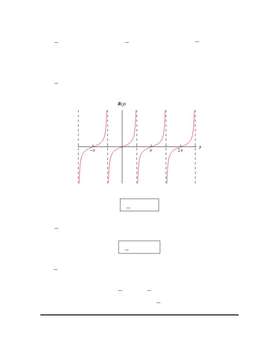
Calculus I

http://tutorial.math.lamar.edu/terms.aspx

(a)

( )

lim

R y

−

→

(b)

( )

lim

R y

→

(c)

( )

lim

R y

→

Hint : Don’t forget the graph of the tangent function.

(a)

( )

lim

R y

−

→

The easiest way to do this problem is from the graph of the tangent function so here is a quick
sketch of the tangent function over several periods.

From the sketch we can see that,

( )

lim tan

−

→

= ∞

(b)

( )

lim

R y

→

From the graph in the first part we can see that,

( )

lim tan

→

= −∞

(c)

( )

lim

R y

→

From the first two parts that,

( )

lim

R y

−

→

≠

and so, from our basic limit properties we can see that

( )

lim

R y

→

does not exist.

Calculus I

http://tutorial.math.lamar.edu/terms.aspx

7. Find all the vertical asymptotes of

( )

(

)

10 3

f x

−

Hint : Remember how vertical asymptotes are defined and use the examples above to help
determine where they are liable to be for the given function. Once you have the locations for the
possible vertical asymptotes verify that they are in fact vertical asymptotes.

Solution
Recall that vertical asymptotes will occur at

if any of the limits (one-sided or overall limit)

are plus or minus infinity.

From previous examples we can see that for rational expressions vertical asymptotes will occur
where there is division by zero. Therefore it looks like the only possible vertical asymptote will

be at

Now let’s verify that this is in fact a vertical asymptote by evaluating the two one-sided limits,

(

)

(

)

lim

and

lim

10 3

−

→

−

In either case as

→

(from both left and right) the numerator goes to

For the one-sided limits we have the following information,

10 3

−

→

⇒

− >

⇒

−

→

⇒

− <

⇒

−

Now, because of the exponent on the denominator is even we can see that for either of the one-
sided limits we will have,

(

)

10 3

−

→

So, in either case, in the limit, the numerator approaches a fixed positive number and the
denominator is positive and increasingly small. Therefore, we will have,

(

)

(

)

(

)

lim

10 3

−

→

= ∞

−

Any of these limits indicate that there is in fact a vertical asymptote at

8. Find all the vertical asymptotes of

( ) ( )( )

g x

−

Calculus I

http://tutorial.math.lamar.edu/terms.aspx

if any of the limits (one-sided or overall limit)

are plus or minus infinity.

From previous examples we can see that for rational expressions vertical asymptotes will occur
where there is division by zero. Therefore it looks like we will have possible vertical asymptote

= −

and

Now let’s verify that these are in fact vertical asymptotes by evaluating the two one-sided limits
for each of them.

Let’s start with

= −

. We’ll need to evaluate,

(

)(

)

(

)(

)

lim

and

lim

−

→−

−

In either case as

→ −

(from both left and right) the numerator is a constant -8.

For the one-sided limits we have the following information,

−

→ −

⇒

< −

⇒

+ <

→ −

⇒

> −

⇒

+ >

Also, note that for x’s close enough to -5 (which because we’re looking at

→ −

is safe

enough to assume), we will have

− <

So, in the left-hand limit, the numerator is a fixed negative number and the denominator is
positive (a product of two negative numbers) and increasingly small. Likewise, for the right-hand
limit, the denominator is negative (a product of a positive and negative number) and increasingly
small. Therefore, we will have,

(

)(

)

(

)(

)

lim

and

lim

−

→−

−

= −∞

= ∞

−

Now for

. Again, the numerator is a constant -8. We also have,

−

→

⇒

− <

→

⇒

− >

Calculus I

http://tutorial.math.lamar.edu/terms.aspx

Finally, for x’s close enough to 9 (which because we’re looking at

→

is safe enough to

assume), we will have

+ >

So, in the left-hand limit, the numerator is a fixed negative number and the denominator is
negative (a product of a positive and negative number) and increasingly small. Likewise, for the
right-hand limit, the denominator is negative (a product of two negative numbers) and
increasingly small. Therefore, we will have,

(

)(

)

(

)(

)

lim

and

lim

−

→

−

= ∞

= −∞

−

So, as all of these limits show we do in fact have vertical asymptotes at

= −

and

Limits At Infinity, Part I

1. For

( )

f x

−

evaluate each of the following limits.

(a)

( )

lim

f x

→−∞

(b)

( )

lim

f x

→∞

(a)

( )

lim

f x

→−∞

To do this all we need to do is factor out the largest power of x from the whole polynomial and
then use basic limit properties along with

Fact 1

from this section to evaluate the limit.

(

)

(

)

( )( )

lim 4

lim

lim 4

→−∞









−

























−

= −∞

















(b)

( )

lim

f x

→∞

For this part all of the mathematical manipulations we did in the first part did not depend upon the
limit itself and so don’t need to be redone here. We can pick up the problem right before we
actually took the limits and then proceed.

(

)

( )

( )( )

lim 4

lim

lim 4

→∞









−

= ∞

















Calculus I

http://tutorial.math.lamar.edu/terms.aspx

2. For

( )

h t

−

evaluate each of the following limits.

(a)

( )

lim

h t

→−∞

(b)

( )

lim

h t

→∞

(a)

( )

lim

h t

→−∞

To do this all we need to do is factor out the largest power of x from the whole polynomial and
then use basic limit properties along with

Fact 1

from this section to evaluate the limit.

Note as well that we’ll convert the root over to a fractional exponent in order to allow it to be
easier to deal with. Also note that this limit is a perfectly acceptable limit because the root is a
cube root and we can take cube roots of negative numbers! We would only have run into
problems had the index on the root been an even number.

( )

( )( )

lim

→−∞





















−









































−

= ∞ − = −∞

















(b)

( )

lim

h t

→∞

( )

( )( )

lim

→∞





















−

= ∞ − = −∞

























3. For

( )

8 4

f x

−

answer each of the following questions.

(a) Evaluate

( )

lim

f x

→−∞

(b) Evaluate

( )

lim

f x

→∞

(c) Write down the equation(s) of any horizontal asymptotes for the function.

Calculus I

http://tutorial.math.lamar.edu/terms.aspx

(a) Evaluate

( )

lim

f x

→−∞

To do this all we need to do is factor out the largest power of x that is in the denominator from
both the denominator and the numerator. Then all we need to do is use basic limit properties
along with

Fact 1

from this section to evaluate the limit.

8 4

lim

→−∞





−





−

















(b) Evaluate

( )

lim

f x

→∞

For this part all of the mathematical manipulations we did in the first part did not depend upon the
limit itself and so don’t really need to be redone here. However, it is easy enough to add them in
so we’ll go ahead and include them.

8 4

lim

→∞





−





−

















(c) Write down the equation(s) of any horizontal asymptotes for the function.

We know that there will be a horizontal asymptote for

→ −∞

( )

lim

f x

→−∞

exists and is a

finite number. Likewise we’ll have a horizontal asymptote for

→ ∞

( )

lim

f x

→∞

exists and is

a finite number.

Therefore, from the first two parts, we can see that we will get the horizontal asymptote,

= −

for both

→ −∞

and

→ ∞

4. For

( )

5 10

f x

−

answer each of the following questions.

(a) Evaluate

( )

lim

f x

→−∞

(b) Evaluate

( )

lim

f x

→∞

(c) Write down the equation(s) of any horizontal asymptotes for the function.

Calculus I

http://tutorial.math.lamar.edu/terms.aspx

(a) Evaluate

( )

lim

f x

→−∞

Fact 1

from this section to evaluate the limit.

lim

5 10

→−∞





− +





−

−∞





= ∞

−





−









(b) Evaluate

( )

lim

f x

→∞

lim

5 10

→∞





− +





−

∞





= −∞

−





−









(c) Write down the equation(s) of any horizontal asymptotes for the function.

We know that there will be a horizontal asymptote for

→ −∞

( )

lim

f x

→−∞

exists and is a

finite number. Likewise we’ll have a horizontal asymptote for

→ ∞

( )

lim

f x

→∞

exists and is

a finite number.

Therefore, from the first two parts, we can see that this function will have no horizontal
asymptotes since neither of the two limits are finite.

5. For

( )

f x

−

answer each of the following questions.

(a) Evaluate

( )

lim

f x

→−∞

(b) Evaluate

( )

lim

f x

→∞

(c) Write down the equation(s) of any horizontal asymptotes for the function.

(a) Evaluate

( )

lim

f x

→−∞

Calculus I

http://tutorial.math.lamar.edu/terms.aspx

Fact 1

from this section to evaluate the limit.

lim

→−∞





−





−

















(b) Evaluate

( )

lim

f x

→∞

lim

→∞





−





−

















(c) Write down the equation(s) of any horizontal asymptotes for the function.

We know that there will be a horizontal asymptote for

→ −∞

( )

lim

f x

→−∞

exists and is a

finite number. Likewise we’ll have a horizontal asymptote for

→ ∞

( )

lim

f x

→∞

exists and is

a finite number.

Therefore, from the first two parts, we can see that we will get the horizontal asymptote,

for both

→ −∞

and

→ ∞

6. For

( )

3 6

f x

−

answer each of the following questions.

(a) Evaluate

( )

lim

f x

→−∞

(b) Evaluate

( )

lim

f x

→∞

(c) Write down the equation(s) of any horizontal asymptotes for the function.

(a) Evaluate

( )

lim

f x

→−∞

Calculus I

http://tutorial.math.lamar.edu/terms.aspx

Fact 1

from this section to evaluate the limit.

lim

3 6

→−∞





−





−





−





−









(b) Evaluate

( )

lim

f x

→∞

lim

3 6

→∞





−





−





−





−









(c) Write down the equation(s) of any horizontal asymptotes for the function.

We know that there will be a horizontal asymptote for

→ −∞

( )

lim

f x

→−∞

exists and is a

finite number. Likewise we’ll have a horizontal asymptote for

→ ∞

( )

lim

f x

→∞

exists and is

a finite number.

Therefore, from the first two parts, we can see that we will get the horizontal asymptote,

for both

→ −∞

and

→ ∞

7. For

( )

f x

−

answer each of the following questions.

(a) Evaluate

( )

lim

f x

→−∞

(b) Evaluate

( )

lim

f x

→∞

(c) Write down the equation(s) of any horizontal asymptotes for the function.

(a) Evaluate

( )

lim

f x

→−∞

Calculus I

http://tutorial.math.lamar.edu/terms.aspx

Fact 1

from this section to evaluate the limit.

lim

→−∞





−





−

















(b) Evaluate

( )

lim

f x

→∞

lim

→∞





−





−

















(c) Write down the equation(s) of any horizontal asymptotes for the function.

We know that there will be a horizontal asymptote for

→ −∞

( )

lim

f x

→−∞

exists and is a

finite number. Likewise we’ll have a horizontal asymptote for

→ ∞

( )

lim

f x

→∞

exists and is

a finite number.

Therefore, from the first two parts, we can see that we will get the horizontal asymptote,

for both

→ −∞

and

→ ∞

8. For

( )

7 9

1 2

f x

−

answer each of the following questions.

(a) Evaluate

( )

lim

f x

→−∞

(b) Evaluate

( )

lim

f x

→∞

(c) Write down the equation(s) of any horizontal asymptotes for the function.

(a) Evaluate

( )

lim

f x

→−∞

Calculus I

http://tutorial.math.lamar.edu/terms.aspx

Fact 1

from this section to evaluate the limit.

In this case the largest power of x in the denominator is just x and so we will need to factor an x
out of both the denominator and the numerator. Recall as well that this means we’ll need to

factor an

out of the root in the numerator so that we’ll have an x in the numerator when we are

done.

So, let’s do the first couple of steps in this process to get us started.

7 9

lim

1 2

→−∞













−













−

























Recall from the discussion in this section that,

and we do need to be careful with that.

Now, because we are looking at the limit

→ −∞

it is safe to assume that

. Therefore,

from the definition of the absolute value we get,

= −

and the limit is then,

7 9

lim

1 2

→−∞

−





−









(b) Evaluate

( )

lim

f x

→∞

For this part all of the mathematical manipulations we did in the first part up to dealing with the
absolute value did not depend upon the limit itself and so don’t really need to be redone here. So,
up to that part we have,

7 9

lim

1 2

→∞

−





−









In this part we are looking at the limit

→ ∞

and so it will be safe to assume in this part that

. Therefore, from the definition of the absolute value we get,

Calculus I

http://tutorial.math.lamar.edu/terms.aspx

and the limit is then,

7 9

lim

1 2

→∞

= −

−





−









(c) Write down the equation(s) of any horizontal asymptotes for the function.

We know that there will be a horizontal asymptote for

→ −∞

( )

lim

f x

→−∞

exists and is a

finite number. Likewise we’ll have a horizontal asymptote for

→ ∞

( )

lim

f x

→∞

exists and is

a finite number.

Therefore, from the first two parts, we can see that we will get the horizontal asymptote,

for

→ −∞

and we have the horizontal asymptote,

= −

for

→ ∞

9. For

( )

f x

answer each of the following questions.

(a) Evaluate

( )

lim

f x

→−∞

(b) Evaluate

( )

lim

f x

→∞

(c) Write down the equation(s) of any horizontal asymptotes for the function.

(a) Evaluate

( )

lim

f x

→−∞

Fact 1

from this section to evaluate the limit.

For the denominator we need to be a little careful. The power of x in the denominator needs to be
outside of the root so it can cancel against the x’s in the numerator. The largest power of x
outside of the root that we can get (and leave something we can deal with in the root) will be just

x. We get this by factoring an

out of the root.

So, let’s do the first couple of steps in this process to get us started.

Calculus I

http://tutorial.math.lamar.edu/terms.aspx

lim

→−∞

















































Recall from the discussion in this section that,

and we do need to be careful with that.

Now, because we are looking at the limit

→ −∞

it is safe to assume that

. Therefore,

from the definition of the absolute value we get,

= −

and the limit is then,

lim

→−∞













−

(b) Evaluate

( )

lim

f x

→∞

lim

→∞













In this part we are looking at the limit

→ ∞

and so it will be safe to assume in this part that

. Therefore, from the definition of the absolute value we get,

and the limit is then,

lim

→∞













(c) Write down the equation(s) of any horizontal asymptotes for the function.

Calculus I

http://tutorial.math.lamar.edu/terms.aspx

We know that there will be a horizontal asymptote for

→ −∞

( )

lim

f x

→−∞

exists and is a

finite number. Likewise we’ll have a horizontal asymptote for

→ ∞

( )

lim

f x

→∞

exists and is

a finite number.

Therefore, from the first two parts, we can see that we will get the horizontal asymptote,

= −

for

→ −∞

and we have the horizontal asymptote,

for

→ ∞

10. For

( )

f x

+ −

answer each of the following questions.

(a) Evaluate

( )

lim

f x

→−∞

(b) Evaluate

( )

lim

f x

→∞

(c) Write down the equation(s) of any horizontal asymptotes for the function.

(a) Evaluate

( )

lim

f x

→−∞

Fact 1

from this section to evaluate the limit.

. We get this by factoring an

out of the root.

So, let’s do the first couple of steps in this process to get us started.

Calculus I

http://tutorial.math.lamar.edu/terms.aspx

lim

→−∞





+ −





+ −

























+ −

















Recall from the discussion in this section that,

So in this case we’ll have,

and note that we can get rid of the absolute value bars because we know that

≥

. So, let’s

finish the limit up.

lim

→−∞





+ −





+ −

−





(b) Evaluate

( )

lim

f x

→∞

Unlike the previous two problems with roots in them all of the mathematical manipulations in this

case did not depend upon the actual limit because we were factoring an

out which will always

be positive and so there will be no reason to redo all of that work.

Here is this limit (with most of the work excluded),

For this part all of the mathematical manipulations we did in the first part up to dealing with the
absolute value did not depend upon the limit itself and so don’t really need to be redone here. So,
up to that part we have,

lim

→∞





+ −





+ −

−





(c) Write down the equation(s) of any horizontal asymptotes for the function.

Calculus I

http://tutorial.math.lamar.edu/terms.aspx

We know that there will be a horizontal asymptote for

→ −∞

( )

lim

f x

→−∞

exists and is a

finite number. Likewise we’ll have a horizontal asymptote for

→ ∞

( )

lim

f x

→∞

exists and is

a finite number.

Therefore, from the first two parts, we can see that we will get the horizontal asymptote,

= −

For both

→ −∞

and

→ ∞

Limits At Infinity, Part II

1. For

( )

8 2

x x

f x

−

= e

evaluate each of the following limits.

(a)

( )

lim

f x

→−∞

(b)

( )

lim

f x

→∞

(a)

( )

lim

f x

→−∞

First notice that,

(

)

lim 8 2

→−∞

−

= ∞

If you aren’t sure about this limit you should go back to the previous section and work some of
the examples there to make sure that you can do these kinds of limits.

Now, recalling

Example 1

from this section, we know that because the exponent goes to infinity

in the limit the answer is,

8 2

lim

x x

−

→−∞

= ∞

(b)

( )

lim

f x

→∞

First notice that,

(

)

lim 8 2

→∞

−

= −∞

If you aren’t sure about this limit you should go back to the previous section and work some of
the examples there to make sure that you can do these kinds of limits.

Calculus I

http://tutorial.math.lamar.edu/terms.aspx

Now, recalling

Example 1

from this section, we know that because the exponent goes to negative

infinity in the limit the answer is,

8 2

lim

x x

−

→∞

2. For

( )

5 3

f x

= e

evaluate each of the following limits.

(a)

( )

lim

f x

→−∞

(b)

( )

lim

f x

→∞

(a)

( )

lim

f x

→−∞

First notice that,

lim

5 3

→−∞

= −∞

If you aren’t sure about this limit you should go back to the previous section and work some of
the examples there to make sure that you can do these kinds of limits.

Now, recalling

Example 1

from this section, we know that because the exponent goes to negative

infinity in the limit the answer is,

5 3

lim

→−∞

(b)

( )

lim

f x

→∞

First notice that,

lim

5 3

→∞

= ∞

If you aren’t sure about this limit you should go back to the previous section and work some of
the examples there to make sure that you can do these kinds of limits.

Now, recalling

Example 1

from this section, we know that because the exponent goes to infinity

in the limit the answer is,

5 3

lim

→∞

= ∞

3. For

( )

f x

−

evaluate each of the following limits.

(a)

( )

lim

f x

→−∞

(b)

( )

lim

f x

→∞

Calculus I

http://tutorial.math.lamar.edu/terms.aspx

Hint : Remember that if there are two terms that seem to be suggesting that the function should be
going in opposite directions that you’ll need to factor out of the function that term that is going to
infinity faster to “prove” the limit.

(a)

( )

lim

f x

→−∞

For this limit the exponentials with positive exponents will simply go to zero and there is only
one exponential with a negative exponent (which will go to infinity) and so there isn’t much to do
with this limit.

(

)

lim 2

−

→−∞

−

= − ∞ − = −∞

(b)

( )

lim

f x

→∞

Here we have two exponents with positive exponents and so both will go to infinity in the limit.
However each term has opposite signs and so each term seems to be suggesting different answers
for the limit.

In order to determine which “wins out” so to speak all we need to do is factor out the term with
the largest exponent and then use basic limit properties.

(

)

(

)

( )( )

lim 2

lim

−

→∞





−

= ∞





4. For

( )

f x

−

evaluate each of the following limits.

(a)

( )

lim

f x

→−∞

(b)

( )

lim

f x

→∞

(a)

( )

lim

f x

→−∞

Here we have two exponents with negative exponents and so both will go to infinity in the limit.
However each term has opposite signs and so each term seems to be suggesting different answers
for the limit.

In order to determine which “wins out” so to speak all we need to do is factor out the term with
the most negative exponent and then use basic limit properties.

(

)

(

)

( )( )

lim 3

lim

−

→−∞





−

− −

= ∞ − = −∞





Calculus I

http://tutorial.math.lamar.edu/terms.aspx

(b)

( )

lim

f x

→∞

For this limit the exponentials with negative exponents will simply go to zero and there is only
one exponential with a positive exponent (which will go to infinity) and so there isn’t much to do
with this limit.

(

)

lim 3

0 0

−

→∞

−

= − − ∞ = −∞

5. For

( )

f x

−

evaluate each of the following limits.

(a)

( )

lim

f x

→−∞

(b)

( )

lim

f x

→∞

Hint : Remember that you’ll need to factor the term in the denominator that is causing the
denominator to go to infinity from both the numerator and denominator in order to evaluate this
limit.

(a)

( )

lim

f x

→−∞

The exponential with the negative exponent is the only term in the denominator going to infinity
for this limit and so we’ll need to factor the exponential with the negative exponent in the
denominator from both the numerator and denominator to evaluate this limit.

(

)

(

)

1 2

1 0

lim

0 7

−

→−∞

−

= −

−

(b)

( )

lim

f x

→∞

The exponential with the positive exponent is the only term in the denominator going to infinity
for this limit and so we’ll need to factor the exponential with the positive exponent in the
denominator from both the numerator and denominator to evaluate this limit.

(

)

(

)

0 2

lim

9 7

9 0

9 7

−

→∞

−

= −

−

6. For

( )

f x

−

evaluate each of the following limits.

(a)

( )

lim

f x

→−∞

(b)

( )

lim

f x

→∞

Calculus I

http://tutorial.math.lamar.edu/terms.aspx

Hint : Remember that you’ll need to factor the term in the denominator that is causing the
denominator to go to infinity fastest from both the numerator and denominator in order to
evaluate this limit.

(a)

( )

lim

f x

→−∞

The exponentials with the negative exponents are the only terms in the denominator going to
infinity for this limit and so we’ll need to factor the exponential with the most negative exponent
in the denominator (because it will be going to infinity fastest) from both the numerator and
denominator to evaluate this limit.

(

)

(

)

lim

0 0

lim

0 0 2

−

→−∞

−

→−∞

−

∞ − −

= ∞

+ +

(b)

( )

lim

f x

→∞

The exponentials with the positive exponents are the only terms in the denominator going to
infinity for this limit and so we’ll need to factor the exponential with the most positive exponent
in the denominator (because it will be going to infinity fastest) from both the numerator and
denominator to evaluate this limit.

(

)

(

)

lim

16 2

0 0 0

lim

16 2

0 16 0

−

→−∞

−

→−∞

−

+ +

−

− −

+ +

7. Evaluate

(

)

lim ln 4 9

→−∞

− −

Solution
First notice that,

(

)

lim 4 9

→−∞

− −

= ∞

If you aren’t sure about this limit you should go back to the previous section and work some of
the examples there to make sure that you can do these kinds of limits.

Now, recalling

Example 5

from this section, we know that because the argument goes to infinity

in the limit the answer is,

(

)

lim ln 4 9

t t

→−∞

− −

= ∞

Calculus I

http://tutorial.math.lamar.edu/terms.aspx

8. Evaluate

lim ln

→−∞





−









Solution
First notice that,

lim

→−∞

−

= ∞

If you aren’t sure about this limit you should go back to the previous section and work some of
the examples there to make sure that you can do these kinds of limits.

Now, recalling

Example 5

from this section, we know that because the argument goes to infinity

in the limit the answer is,

lim ln

→−∞





−

= ∞









9. Evaluate

11 8

lim ln

→∞













Solution
First notice that,

11 8

lim

→∞

If you aren’t sure about this limit you should go back to the previous section and work some of
the examples there to make sure that you can do these kinds of limits.

Also, note that because we are evaluating the limit

→ ∞

it is safe to assume that

and so

we can further say that,

11 8

→

Now, recalling

Example 5

from this section, we know that because the argument goes to zero

from the right in the limit the answer is,

11 8

lim ln

→∞



 = −∞









10. Evaluate

(

)

lim tan

−

→−∞

− +

Calculus I

http://tutorial.math.lamar.edu/terms.aspx

Solution
First notice that,

(

)

lim 7

→−∞

− +

= −∞

If you aren’t sure about this limit you should go back to the previous section and work some of
the examples there to make sure that you can do these kinds of limits.

Now, recalling

Example 7

from this section, we know that because the argument goes to negative

infinity in the limit the answer is,

(

)

lim tan

−

→−∞

− +

= −

11. Evaluate

4 7

lim tan

−

→∞









−





Solution
First notice that,

4 7

lim

→∞

= −

−

If you aren’t sure about this limit you should go back to the previous section and work some of
the examples there to make sure that you can do these kinds of limits.

Then answer is then,

( )

4 7

lim tan

tan

−

→∞



 =

−





−





Do not get so used the “special case” limits that we tend to usually do in the problems at the end
of a section that you decide that you must have done something wrong when you run across a
problem that doesn’t fall in the “special case” category.

12. Evaluate

lim tan

w w

−

→∞





−





−





Solution
First notice that,

lim

w w

→∞

−

= ∞

−

If you aren’t sure about this limit you should go back to the previous section and work some of
the examples there to make sure that you can do these kinds of limits.

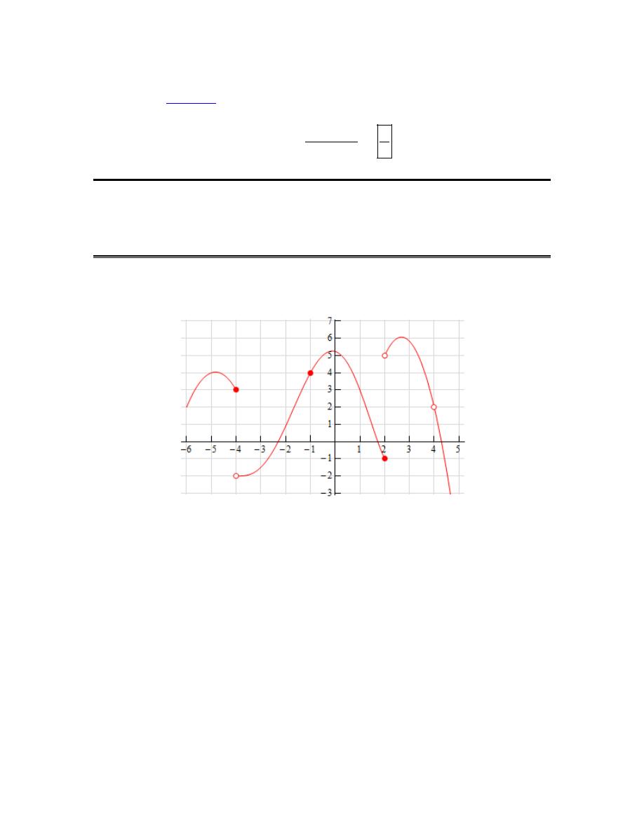
Calculus I

http://tutorial.math.lamar.edu/terms.aspx

Now, recalling

Example 7

from this section, we know that because the argument goes to infinity

in the limit the answer is,

lim tan

w w

−

→∞





−





−





Continuity

1. The graph of

( )

f x

is given below. Based on this graph determine where the function is

discontinuous.

Solution

Before starting the solution recall that in order for a function to be continuous at

both

( )

f a

and

( )

lim

f x

→

must exist and we must have,

( )

lim

f x

f a

→

Using this idea it should be fairly clear where the function is not continuous.

First notice that at

= −

we have,

( )

lim

f x

−

→−

= ≠ − =

and therefore we also know that

( )

lim

f x

→−

doesn’t exist. We can therefore conclude that

( )

f x

is discontinuous at

= −

because the limit does not exist.

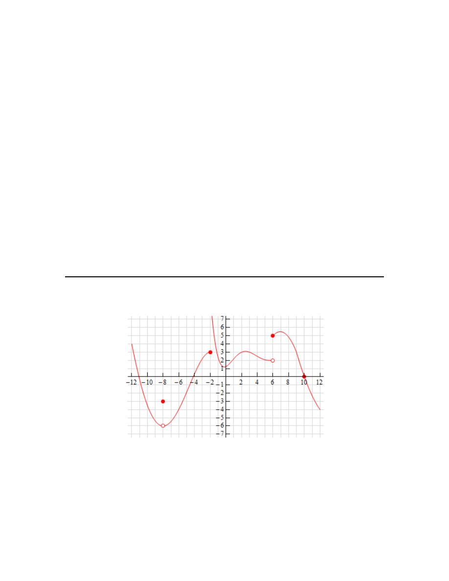
Calculus I

http://tutorial.math.lamar.edu/terms.aspx

Likewise, at

we have,

( )

lim

1 5

lim

f x

−

→

= − ≠ =

and therefore we also know that

( )

lim

f x

→

doesn’t exist. So again, because the limit does not

exist, we can see that

( )

f x

is discontinuous at

Finally let’s take a look at

. Here we can see that,

( )

lim

f x

−

→

= =

and therefore we also know that

( )

lim

f x

→

. However, we can also see that

( )

doesn’t

exist and so once again

( )

f x

is discontinuous at

because this time the function does not

exist at

All other points on this graph will have both the function and limit exist and we’ll have

( )

lim

f x

f a

→

and so will be continuous.

In summary then the points of discontinuity for this graph are :

= −

and

2. The graph of

( )

f x

is given below. Based on this graph determine where the function is

discontinuous.

Solution

Before starting the solution recall that in order for a function to be continuous at

both

( )

f a

and

( )

lim

f x

→

must exist and we must have,

( )

lim

f x

f a

→

Calculus I

http://tutorial.math.lamar.edu/terms.aspx

Using this idea it should be fairly clear where the function is not continuous.

First notice that at

= −

we have,

( )

lim

f x

−

→−

= − =

and therefore we also know that

( )

lim

f x

→−

= −

. We can also see that

( )

− = −

and so we

have,

( )

lim

f x

→−

− =

≠

− = −

Because the function and limit have different values we can conclude that

( )

f x

discontinuous at

= −

Next let’s take a look at

= −

we have,

( )

lim

f x

−

→−

= ≠ ∞ =

and therefore we also know that

( )

lim

f x

→−

doesn’t exist. We can therefore conclude that

( )

f x

is discontinuous at

= −

because the limit does not exist.

Finally let’s take a look at

. Here we can see we have,

( )

lim

f x

−

→

= ≠ =

and therefore we also know that

( )

lim

f x

→

doesn’t exist. So, once again, because the limit does

not exist, we can conclude that

( )

f x

is discontinuous at

All other points on this graph will have both the function and limit exist and we’ll have

( )

lim

f x

f a

→

and so will be continuous.

In summary then the points of discontinuity for this graph are :

= −

and

3. Using only Properties 1- 9 from the

Limit Properties

section, one-sided limit properties (if

needed) and the definition of continuity determine if the following function is continuous or

discontinuous at (a)

= −

, (b)

, (c)

( )

9 3

f x

−

(a)

= −

Before starting off with the solution to this part notice that we CAN NOT do what we’ve
commonly done to evaluate limits to this point. In other words, we can’t just plug in the point to

Calculus I

http://tutorial.math.lamar.edu/terms.aspx

evaluate the limit. Doing this implicitly assumes that the function is continuous at the point and
that is what we are being asked to determine here.

Therefore the only way for us to compute the limit is to go back to the properties from the Limit
Properties section and compute the limit as we did back in that section. We won’t be putting all
the details here so if you need a little refresher on doing this you should go back to the problems
from that section and work a few of them.

So, here we go.

( )

(

)

(

)

( )

lim 4

4 lim

lim 5

lim

9 3

lim 9 3

lim 9 3 lim

9 3

f x

→−

− +

−

− −

So, we can see that

( )

lim

f x

→−

−

and so the function is continuous at

= −

(b)

For justification on why we can’t just plug in the number here check out the comment at the
beginning of the solution to (a).

Here is the work for this part.

( )

(

)

(

)

( )

lim 4

4 lim

lim 5

4 0

lim

9 3

lim 9 3

lim 9 3lim

9 3 0

f x

→

−

So, we can see that

( )

lim

f x

→

and so the function is continuous at

(c)

For justification on why we can’t just plug in the number here check out the comment at the

beginning of the solution to (a). Although there is also of course the problem here that

( )

doesn’t exist and so we couldn’t plug in the value even if we wanted to.

This also tells us what we need to know however. As noted in the notes for this section if either
the function or the limit do not exist then the function is not continuous at the point. Therefore

we can see that the function is not continuous at

For practice you might want to verify that,

( )

lim

f x

−

→

= ∞

= −∞

and so

( )

lim

f x

→

also doesn’t exist.

Calculus I

http://tutorial.math.lamar.edu/terms.aspx

4. Using only Properties 1- 9 from the

Limit Properties

section, one-sided limit properties (if

needed) and the definition of continuity determine if the following function is continuous or

discontinuous at (a)

= −

, (b)

, (c)

( )

g z

−

(a)

= −

Of course even if we had tried to plug in the point we would have run into problems as

( )

−

doesn’t exist and this tell us all we need to know. As noted in the notes for this section if either
the function or the limit do not exist then the function is not continuous at the point. Therefore

we can see that the function is not continuous at

= −

For practice you might want to verify that,

( )

lim

g z

−

→−

= ∞

= −∞

and so

( )

lim

g z

→−

also doesn’t exist.

(b)

For justification on why we can’t just plug in the number here check out the comment at the
beginning of the solution to (a).

Therefore, because we can’t just plug the point into the function, the only way for us to compute
the limit is to go back to the properties from the Limit Properties section and compute the limit as
we did back in that section. We won’t be putting all the details here so if you need a little
refresher on doing this you should go back to the problems from that section and work a few of
them.

Here is the work for this part.

( )

(

)

( )

lim 6

lim

3lim

lim10

lim

3 0

g z

→

−

So, we can see that

( )

lim

g x

→

and so the function is continuous at

Calculus I

http://tutorial.math.lamar.edu/terms.aspx

(c)

For justification on why we can’t just plug in the number here check out the comment at the

beginning of the solution to (a). Although there is also of course the problem here that

( )

doesn’t exist and so we couldn’t plug in the value even if we wanted to.

This also tells us what we need to know however. As noted in the notes for this section if either
the function of the limit do not exist then the function is not continuous at the point. Therefore

we can see that the function is not continuous at

For practice you might want to verify that,

( )

lim

g z

−

→

= −∞

= ∞

and so

( )

lim

g z

→

also doesn’t exist.

5. Using only Properties 1- 9 from the

Limit Properties

section, one-sided limit properties (if

needed) and the definition of continuity determine if the following function is continuous or

discontinuous at (a)

, (b)

( )

g x



= 

−

≥



(a)

For this part we can notice that because there are values of x on both sides of

in the range

we won’t need to worry about one-sided limits here. Here is the work for this part.

( )

lim

lim 2

2 lim

2 4

g x

→

So, we can see that

( )

lim

g x

→

and so the function is continuous at

(b)

Calculus I

http://tutorial.math.lamar.edu/terms.aspx

For justification on why we can’t just plug in the number here check out the comment at the
beginning of the solution to (a).

For this part we have the added complication that the point we’re interested in is also the “cut-
off” point of the piecewise function and so we’ll need to take a look at the two one sided limits to
compute the overall limit and again because we are being asked to determine if the function is
continuous at this point we’ll need to resort to basic limit properties to compute the one-sided
limits and not just plug in the point (which assumes continuity again…).

Here is the work for this part.

( )

(

)

lim

lim 2

2 lim

2 6

lim

lim 1

6 1 5

g x

−

→

− =

−

= − =

So we can see that,

( )

lim

g x

−

→

≠

and so

( )

lim

g x

→

does not exist.

Now, as discussed in the notes for this section, in order for a function to be continuous at a point

both the function and the limit must exist. Therefore this function is not continuous at

because

( )

lim

g x

→

does not exist.

6. Using only Properties 1- 9 from the

Limit Properties

section, one-sided limit properties (if

needed) and the definition of continuity determine if the following function is continuous or

discontinuous at (a)

= −

, (b)

( )

h t



< −

= 

≥ −



(a)

= −

Before starting off with the solution to this part notice that we CAN NOT do what we’ve
commonly done to evaluate limits to this point. In other words, we can’t just plug in the point to
evaluate the limit. Doing this implicitly assumes that the function is continuous at the point and
that is what we are being asked to determine here.

Therefore the only way for us to compute the limit is to go back to the properties from the Limit
Properties section and compute the limit as we did back in that section. We won’t be putting all
the details here so if you need a little refresher on doing this you should go back to the problems
from that section and work a few of them.

Also notice that for this part we have the added complication that the point we’re interested in is
also the “cut-off” point of the piecewise function and so we’ll need to take a look at the two one

Calculus I

http://tutorial.math.lamar.edu/terms.aspx

sided limits to compute the overall limit and again because we are being asked to determine if the
function is continuous at this point we’ll need to resort to basic limit properties to compute the
one-sided limits and not just plug in the point (which assumes continuity again…).

Here is the work for this part.

( )

(

)

lim

lim 6

2 6

h t

g t

−

→−

= −

= − + =

So we can see that,

( )

lim

h t

−

→−

and so

( )

lim

h t

→−

Next, a quick computation shows us that

( )

2 6

− = − + =

and so we can see that

( )

lim

h t

→−

−

and so the function is continuous at

= −

(b)

For justification on why we can’t just plug in the number here check out the comment at the
beginning of the solution to (a).

For this part we can notice that because there are values of t on both sides of

in the range

≥ −

we won’t need to worry about one-sided limits here. Here is the work for this part.

Here is the work for this part.

( )

(

)

( )

lim

lim 6 10 6

h t

→

+ =

So, we can see that

( )

lim

h t

→

and so the function is continuous at

7. Using only Properties 1- 9 from the

Limit Properties

section, one-sided limit properties (if

needed) and the definition of continuity determine if the following function is continuous or

discontinuous at (a)

= −

, (b)

( )

1 3

g x

−

< −





= −



− < <





−



(a)

= −

Calculus I

http://tutorial.math.lamar.edu/terms.aspx

( )

(

)

( )

lim

lim 1 3

lim 1 3 lim

1 3

lim

216

g x

−

→−

−

= − − =

= −

So we can see that,

( )

lim

g x

−

→−

≠

and so

( )

lim

g x

→−

does not exist.

Now, as discussed in the notes for this section, in order for a function to be continuous at a point

both the function and the limit must exist. Therefore this function is not continuous at

= −

because

( )

lim

g x

→−

does not exist.

(b)

For justification on why we can’t just plug in the number here check out the comment at the
beginning of the solution to (a).

Again note that we are dealing with another “cut-off” point here so we’ll need to use one-sided
limits again as we did in the previous part.

Here is the work for this part.

( )

(

)

lim

lim 2

lim

2 1 1

g x

−

→

= =

−

= − =

So we can see that,

( )

lim

g x

−

→

and so

( )

lim

g x

→

Calculus I

http://tutorial.math.lamar.edu/terms.aspx

Next, a quick computation shows us that

( )

and so we can see that

( )

lim

g x

→

and

so the function is continuous at

8. Determine where the following function is discontinuous.

( )

f x

−

Hint : If we have two continuous functions and form a rational expression out of them recall
where the rational expression will be discontinuous. We discussed this in the Limit Properties
section, although we were using the phrase “nice enough” there instead of the word “continuity”.

Solution
As noted in the hint for this problem when dealing with a rational expression in which both the
numerator and denominator are continuous (as we have here since both are polynomials) the only
points in which the rational expression will be discontinuous will be where we have division by
zero.

Therefore, all we need to do is determine where the denominator is zero and that is fairly easy for
this problem.

(

)(

)

− =

−

⇒

= −

The function will therefore be discontinuous at the points :

and

= −

9. Determine where the following function is discontinuous.

( )

R t

− −

Calculus I

http://tutorial.math.lamar.edu/terms.aspx

points in which the rational expression will be discontinuous will be where we have division by
zero.

Therefore, all we need to do is determine where the denominator is zero and that is fairly easy for
this problem.

( )

( )( )

( )

4 1

0.10977, 9.10977

2 1

−

− − =

⇒

= −

The function will therefore be discontinuous at the points :

10. Determine where the following function is discontinuous.

( )

2 4 cos 3

h z

−

Hint : If we have two continuous functions and form a rational expression out of them recall
where the rational expression will be discontinuous. We discussed this in the Limit Properties
section, although we were using the phrase “nice enough” there instead of the word “continuity”.

Solution
As noted in the hint for this problem when dealing with a rational expression in which both the
numerator and denominator are continuous (as we have here since the numerator is just a constant
and the denominator is a sum of continuous functions) the only points in which the rational
expression will be discontinuous will be where we have division by zero.

Therefore, all we need to do is determine where the denominator is zero. If you don’t recall how
to solve equations involving trig functions you should go back to the Review chapter and take a
look at the Solving Trig Equations sections there.

Here is the solution work for determining where the denominator is zero. Using our calculator
we get,

( )

2 4 cos 3

cos

1.0472

−

 

−

→

 

 

The second angle will be in the fourth quadrant and is

1.0472

5.2360

−

The denominator will therefore be zero at,

Calculus I

http://tutorial.math.lamar.edu/terms.aspx

1.0472 2

5.2360 2

0, 1, 2,

0.3491

1.7453

0, 1, 2,

= ± ±



The function will therefore be discontinuous at the points,

0.3491

1.7453

0, 1, 2,

= ± ± 

Note as well that this was one of the few trig equations that could be solved exactly if you know
you basic unit circle values. Here is the exact solution for the points of discontinuity.

0, 1, 2,

= +

= ± ± 

11. Determine where the following function is discontinuous.

( )

y x

− e

Hint : If we have two continuous functions and form a rational expression out of them recall
where the rational expression will be discontinuous. We discussed this in the Limit Properties
section, although we were using the phrase “nice enough” there instead of the word “continuity”.

Solution
As noted in the hint for this problem when dealing with a rational expression in which both the
numerator and denominator are continuous (as we have here since the numerator is a polynomial
and the denominator is a sum of two continuous functions) the only points in which the rational
expression will be discontinuous will be where we have division by zero.

Therefore, all we need to do is determine where the denominator is zero and that is fairly easy for
this problem.

( )

(

)

ln 7

0.5270

−

→

+ =

⇒

− = −

The function will therefore be discontinuous at :

( )

(

)

ln 7

0.5270

− = −

12. Determine where the following function is discontinuous.

( )

tan 2

g x

Calculus I

http://tutorial.math.lamar.edu/terms.aspx

( )

sin 2

cos 2

g x

we can see that we really do have a rational expression here. Therefore, all we need to do is
determine where the denominator (i.e. cosine) is zero. If you don’t recall how to solve equations
involving trig functions you should go back to the Review chapter and take a look at the Solving
Trig Equations sections there.

Here is the solution work for determining where the denominator is zero. Using our basic unit
circle knowledge we know where cosine will be zero so we have,

0, 1, 2,

= +

= ± ± 

The denominator will therefore be zero, and the function will be discontinuous, at,

0, 1, 2,

= +

= ± ± 

13. Use the Intermediate Value Theorem to show that

25 8

−

has at least one root in

the interval

[

]

2, 4

−

. Note that you are NOT asked to find the solution only show that at least one

must exist in the indicated interval,

Hint : The hardest part of these problems for most students is just getting started.

First, you need to determine the value of “M” that you need to use and then actually use the
Intermediate Value Theorem. So, go back to the IVT and compare the conclusions of the
theorem and it should be pretty obvious what the M should be and then just check that the
hypothesis (i.e. the “requirements” of the theorem) are met and you’ll pretty much be done.

Solution
Okay, let’s start off by defining,

Calculus I

http://tutorial.math.lamar.edu/terms.aspx

( )

25 8

f x

−

The problem is then asking us to show that there is a c in

[

]

2, 4

−

so that,

( )

f c

= =

but this is exactly the second conclusion of the Intermediate Value Theorem. So, let’s see that the
“requirements” of the theorem are met.

First, the function is a polynomial and so is continuous everywhere and in particular is continuous

on the interval

[

]

2, 4

−

. Note that this IS a requirement that MUST be met in order to use the IVT

and it is the one requirement that is most often overlooked. If we don’t have a continuous
function the IVT simply can’t be used.

Now all that we need to do is verify that M is between the function values as the endpoints of the
interval. So,

( )

167

− =

= −

Therefore we have,

( )

167

0 1

= −

< < =

−

So by the Intermediate Value Theorem there must be a number c such that,

( )

f c

− < <

and we have shown what we were asked to show.

14. Use the Intermediate Value Theorem to show that

(

)

4 ln 5

−

has at least one root

in the interval

[ ]

0, 4

. Note that you are NOT asked to find the solution only show that at least

one must exist in the indicated interval,

Hint : The hardest part of these problems for most students is just getting started.

First, you need to determine the value of “M” that you need to use and then actually use the
Intermediate Value Theorem. So, go back to the IVT and compare the conclusions of the
theorem and it should be pretty obvious what the M should be and then just check that the
hypothesis (i.e. the “requirements” of the theorem) are met and you’ll pretty much be done.

Solution
Okay, let’s start off by defining,

( )

(

)

4 ln 5

f w

−

Calculus I

http://tutorial.math.lamar.edu/terms.aspx

The problem is then asking us to show that there is a c in

[

]

2, 4

−

so that,

( )

f c

= =

but this is exactly the second conclusion of the Intermediate Value Theorem. So, let’s see that the
“requirements” of the theorem are met.

First, the function is a sum of a polynomial (which is continuous everywhere) and a natural

logarithm (which is continuous on

2
5

> −

- i.e. where the argument is positive) and so is

continuous on the interval

[ ]

0, 4

. Note that this IS a requirement that MUST be met in order to

use the IVT and it is the one requirement that is most often overlooked. If we don’t have a
continuous function the IVT simply can’t be used.

Now all that we need to do is verify that M is between the function values as the endpoints of the
interval. So,

( )

2.7726

3.6358

= −

Therefore we have,

( )

2.7726

3.6358

= −

< <

So by the Intermediate Value Theorem there must be a number c such that,

( )

f c

< <

and we have shown what we were asked to show.

15. Use the Intermediate Value Theorem to show that

−

has at least one root in

the interval

[ ]

1, 3

. Note that you are NOT asked to find the solution only show that at least one

( )

f t

= +

−

Calculus I

http://tutorial.math.lamar.edu/terms.aspx

The problem is then asking us to show that there is a c in

[

]

2, 4

−

so that,

( )

f c

= =

but this is exactly the second conclusion of the Intermediate Value Theorem. So, let’s see that the
“requirements” of the theorem are met.

First, the function is a sum and difference of a polynomial and two exponentials (all of which are

continuous everywhere) and so is continuous on the interval

[ ]

1, 3

. Note that this IS a

requirement that MUST be met in order to use the IVT and it is the one requirement that is most
often overlooked. If we don’t have a continuous function the IVT simply can’t be used.

Now all that we need to do is verify that M is between the function values as the endpoints of the
interval. So,

( )

23.7938

190.5734

= −

Therefore we have,

( )

190.5734

23.7938

= −

< <

So by the Intermediate Value Theorem there must be a number c such that,

( )

f c

< <

and we have shown what we were asked to show.

The Definition of the Limit

1. Use the definition of the limit to prove the following limit.

lim

→

Step 1
First, let’s just write out what we need to show.

Let

be any number. We need to find a number

so that,

whenever

− <

< − <

Calculus I

http://tutorial.math.lamar.edu/terms.aspx

This problem can look a little tricky since the two inequalities both involve

−

. Just keep in

mind that the first one is really

( )

f x

− <

where

( )

f x

and

and the second is

really

x a

< − <

where

Step 2
In this case, despite the “trickiness” of the statement we need to prove in Step 1, this is really a
very simple problem.

We need to determine a

that will allow us to prove the statement in Step 1. However, because

both inequalities involve exactly the same absolute value statement so all we need to do is choose

δ ε

Step 3
So, let’s see if this works.

Start off by first assuming that

is any number and choose

δ ε

. We can now assume that

δ ε

< − < =

⇒

< − <

However, if we just look at the right portion of the double inequality we see that this assumption
tells us that,

− <

which is exactly what we needed to show give our choice of

Therefore, according to the definition of the limit we have just proved that,

lim

→

2. Use the definition of the limit to prove the following limit.

(

)

lim

→−

Step 1
First, let’s just write out what we need to show.

Let

be any number. We need to find a number

so that,

Calculus I

http://tutorial.math.lamar.edu/terms.aspx

(

)

( )

whenever

+ − <

< − − <

Or, with a little simplification this becomes,

whenever

+ <

< + <

Step 2
This problem is very similar to Problem 1 from this point on.

We need to determine a

that will allow us to prove the statement in Step 1. However, because

both inequalities involve exactly the same absolute value statement all we need to do is choose

δ ε

Step 3
So, let’s see if this works.

Start off by first assuming that

is any number and choose

δ ε

. We can now assume

that,

( )

δ ε

< − − < =

⇒

< + <

This gives,

(

)

simplify things up a little

using the information we got by assuming

δ ε

+ − = +

So, we’ve shown that,

(

)

( )

whenever

− <

< − − <

and so by the definition of the limit we have just proved that,

(

)

lim

→−

3. Use the definition of the limit to prove the following limit.

lim

→

Calculus I

http://tutorial.math.lamar.edu/terms.aspx

Step 1
First, let’s just write out what we need to show.

Let

be any number. We need to find a number

so that,

whenever

− <

< − <

Step 2
Let’s start with a little simplification of the first inequality.

(

)(

)

− =

−

= +

− <

We have the

−

we expect to see but we also have an

that we’ll need to deal with.

Step 3

To deal with the

let’s first assume that

− <

As we noted in a similar example in the notes for this section this is a legitimate assumption

because the limit is

→

and so x’s will be getting very close to 2. Therefore, provided x is

close enough to 2 we will have

− <

Starting with this assumption we get that,

2 1

− < − <

→

< <

If we now add 2 to all parts of this inequality we get,

< + <

Noticing that 3 > 0 we can see that we then also know that

+ >

and so provided

− <

we will have

+ = +

All this means is that, provided

− <

, we will also have,

+ = + <

→

+ <

This in turn means that we have,

Calculus I

http://tutorial.math.lamar.edu/terms.aspx

because 2

− <

−

+ <

Therefore, if we were to further assume, for some reason, that we wanted

− <

this would

tell us that,

− <

Step 4

Okay, even though it doesn’t seem like it we actually have enough to make a choice for

Given any number

let’s chose

min 1,













Again, this means that

will be the smaller of the two values which in turn means that,

AND

≤

Now assume that

min 1,





< − < =









Step 5
So, let’s see if this works.

Given the assumption

min 1,





< − < =









we know two things. First we know that

− <

. Second we also know that

− <

which in turn implies that

+ <

as we

saw in Step 3.

Now, let’s do the following,

factoring

because we know

− = +

−

+ <

 

− <

 

 

Calculus I

http://tutorial.math.lamar.edu/terms.aspx

So, we’ve shown that,

whenever

min 1,





− <

< − <









and so by the definition of the limit we have just proved that,

lim

→

4. Use the definition of the limit to prove the following limit.

(

)

lim

→−

+ = −

Step 1
First, let’s just write out what we need to show.

Let

be any number. We need to find a number

so that,

( )

whenever

+ − − <

< − − <

Simplifying this a little gives,

whenever

+ <

< + <

Step 2
Let’s start with a little simplification of the first inequality.

(

)(

)

+ =

= +

+ <

We have the

we expect to see but we also have an

that we’ll need to deal with.

Step 3

To deal with the

let’s first assume that

+ <

Calculus I

http://tutorial.math.lamar.edu/terms.aspx

As we noted in a similar example in the notes for this section this is a legitimate assumption

because the limit is

→ −

and so x’s will be getting very close to -3. Therefore, provided x is

close enough to -3 we will have

+ <

Starting with this assumption we get that,

3 1

− < + <

→

− < < −

If we now add 1 to all parts of this inequality we get,

− < + < −

Noticing that -1 < 0 we can see that we then also know that

1 0

+ <

and so provided

+ <

we will have

(

)

+ = − +

. Also from the inequality above we see that,

(

)

< − + <

All this means is that, provided

+ <

, we will also have,

(

)

+ = − + <

→

+ <

This in turn means that we have,

because 1

+ <

Therefore, if we were to further assume, for some reason, that we wanted

+ <

this would

tell us that,

+ <

Step 4

Okay, even though it doesn’t seem like it we actually have enough to make a choice for

Given any number

let’s chose

min 1,













Again, this means that

will be the smaller of the two values which in turn means that,

Calculus I

http://tutorial.math.lamar.edu/terms.aspx

AND

≤

Now assume that

min 1,





< + < =









Step 5
So, let’s see if this works.

Given the assumption

min 1,





< + < =









we know two things. First we know that

+ <

. Second we also know that

+ <

which in turn implies that

+ <

as we

saw in Step 3.

Now, let’s do the following,

factoring

because we know

+ = +

+ <

 

+ <

 

 

So, we’ve shown that,

whenever

min 1,





+ <

< + <









and so by the definition of the limit we have just proved that,

(

)

lim

→−

+ = −

5. Use the definition of the limit to prove the following limit.

(

)

lim

→

= ∞

−

Calculus I

http://tutorial.math.lamar.edu/terms.aspx

Step 1
First, let’s just write out what we need to show.

Let

be any number. We need to find a number

so that,

(

)

whenever

< − <

−

Step 2
Let’s do a little rewrite the first inequality above a little bit.

(

)

(

)

→

−

→

− <

−

From this it looks like we can choose

δ =

Step 3
So, let’s see if this works.

We’ll start by assuming that

is any number and chose

δ =

. We can now assume

that,

< − < =

⇒

< − <

So, if we start with the second inequality we get,

(

)

(

)

(

)

squaring both sides

because 1

rewriting things a little bit

− <

−

So, we’ve shown that,

Calculus I

http://tutorial.math.lamar.edu/terms.aspx

(

)

whenever

< − <

−

and so by the definition of the limit we have just proved that,

(

)

lim

→

= ∞

−

6. Use the definition of the limit to prove the following limit.

lim

−

→

= −∞

Step 1
First, let’s just write out what we need to show.

Let

be any number. Remember that because our limit is going to negative infinity here

we need N to be negative. Now, we need to find a number

so that,

whenever

− < − <

Step 2
Let’s do a little rewrite on the first inequality above to get,

→

Now, keep in mind that N is negative and so

is also negative. From this it looks like we can

choose

= −

. Again, because N is negative this makes

positive, which we need!

Step 3
So, let’s see if this works.

We’ll start by assuming that

is any number and chose

= −

. We can now assume

that,

Calculus I

100

http://tutorial.math.lamar.edu/terms.aspx

− < − <

⇒

< <

So, if we start with the second inequality we get,

rewriting things a little bit

So, we’ve shown that,

whenever

< <

and so by the definition of the limit we have just proved that,

lim

−

→

= −∞

7. Use the definition of the limit to prove the following limit.

lim

→∞

Step 1
First, let’s just write out what we need to show.

Let

be any number. We need to find a number

so that,

whenever

− <

Or, with a little simplification this becomes,

whenever

Calculus I

101

http://tutorial.math.lamar.edu/terms.aspx

Step 2
Let’s start with the inequality on the left and do a little rewriting on it.

→

From this it looks like we can choose

Step 3
So, let’s see if this works.

Start off by first assuming that

is any number and choose

. We can now assume

that,

Starting with this inequality we get,

do a little rewrite

square both sides

because

So, we’ve shown that,

whenever

− <

and so by the definition of the limit we have just proved that,

lim

→∞

Calculus I

102

http://tutorial.math.lamar.edu/terms.aspx