
CALCULUS I
Limits
Paul Dawkins

Calculus I
© 2007 Paul Dawkins
i
http://tutorial.math.lamar.edu/terms.aspx
Table of Contents
Preface ............................................................................................................................................ ii
Limits .............................................................................................................................................. 2
Introduction ................................................................................................................................................ 3
Rates of Change and Tangent Lines ........................................................................................................... 4
The Limit ..................................................................................................................................................13
One-Sided Limits ......................................................................................................................................23
Limit Properties.........................................................................................................................................29
Computing Limits .....................................................................................................................................35
Infinite Limits ...........................................................................................................................................43
Limits At Infinity, Part I............................................................................................................................53
Limits At Infinity, Part II ..........................................................................................................................62
Continuity .................................................................................................................................................72
The Definition of the Limit .......................................................................................................................79

Calculus I
© 2007 Paul Dawkins
ii
http://tutorial.math.lamar.edu/terms.aspx
Preface
Here are my online notes for my Calculus I course that I teach here at Lamar University. Despite
the fact that these are my “class notes”, they should be accessible to anyone wanting to learn
Calculus I or needing a refresher in some of the early topics in calculus.
I’ve tried to make these notes as self contained as possible and so all the information needed to
read through them is either from an Algebra or Trig class or contained in other sections of the
notes.
Here are a couple of warnings to my students who may be here to get a copy of what happened on
a day that you missed.
1. Because I wanted to make this a fairly complete set of notes for anyone wanting to learn
calculus I have included some material that I do not usually have time to cover in class
and because this changes from semester to semester it is not noted here. You will need to
find one of your fellow class mates to see if there is something in these notes that wasn’t
covered in class.
2. Because I want these notes to provide some more examples for you to read through, I
don’t always work the same problems in class as those given in the notes. Likewise, even
if I do work some of the problems in here I may work fewer problems in class than are
presented here.
3. Sometimes questions in class will lead down paths that are not covered here. I try to
anticipate as many of the questions as possible when writing these up, but the reality is
that I can’t anticipate all the questions. Sometimes a very good question gets asked in
class that leads to insights that I’ve not included here. You should always talk to
someone who was in class on the day you missed and compare these notes to their notes
and see what the differences are.
4. This is somewhat related to the previous three items, but is important enough to merit its
own item. THESE NOTES ARE NOT A SUBSTITUTE FOR ATTENDING CLASS!!
Using these notes as a substitute for class is liable to get you in trouble. As already noted
not everything in these notes is covered in class and often material or insights not in these
notes is covered in class.
Limits

Calculus I
© 2007 Paul Dawkins
3
http://tutorial.math.lamar.edu/terms.aspx
Introduction
The topic that we will be examining in this chapter is that of Limits. This is the first of three
major topics that we will be covering in this course. While we will be spending the least amount
of time on limits in comparison to the other two topics limits are very important in the study of
Calculus. We will be seeing limits in a variety of places once we move out of this chapter. In
particular we will see that limits are part of the formal definition of the other two major topics.
Here is a quick listing of the material that will be covered in this chapter.
Tangent Lines and Rates of Change
– In this section we will take a look at two problems that
we will see time and again in this course. These problems will be used to introduce the topic of
limits.
The Limit
– Here we will take a conceptual look at limits and try to get a grasp on just what they
are and what they can tell us.
One-Sided Limits
– A brief introduction to one-sided limits.
Limit Properties
– Properties of limits that we’ll need to use in computing limits. We will also
compute some basic limits in this section
Computing Limits
– Many of the limits we’ll be asked to compute will not be “simple” limits.
In other words, we won’t be able to just apply the properties and be done. In this section we will
look at several types of limits that require some work before we can use the limit properties to
compute them.
Infinite Limits
– Here we will take a look at limits that have a value of infinity or negative
infinity. We’ll also take a brief look at vertical asymptotes.
Limits At Infinity, Part I
– In this section we’ll look at limits at infinity. In other words, limits
in which the variable gets very large in either the positive or negative sense. We’ll also take a
brief look at horizontal asymptotes in this section. We’ll be concentrating on polynomials and
rational expression involving polynomials in this section.
Limits At Infinity, Part II
– We’ll continue to look at limits at infinity in this section, but this
time we’ll be looking at exponential, logarithms and inverse tangents.
Continuity
– In this section we will introduce the concept of continuity and how it relates to
limits. We will also see the Mean Value Theorem in this section.
The Definition of the Limit
– We will give the exact definition of several of the limits covered
in this section. We’ll also give the exact definition of continuity.
Calculus I
© 2007 Paul Dawkins
4
http://tutorial.math.lamar.edu/terms.aspx
Rates of Change and Tangent Lines
In this section we are going to take a look at two fairly important problems in the study of
calculus. There are two reasons for looking at these problems now.
First, both of these problems will lead us into the study of limits, which is the topic of this chapter
after all. Looking at these problems here will allow us to start to understand just what a limit is
and what it can tell us about a function.
Secondly, the rate of change problem that we’re going to be looking at is one of the most
important concepts that we’ll encounter in the second chapter of this course. In fact, it’s probably
one of the most important concepts that we’ll encounter in the whole course. So looking at it now
will get us to start thinking about it from the very beginning.
Tangent Lines
The first problem that we’re going to take a look at is the tangent line problem. Before getting
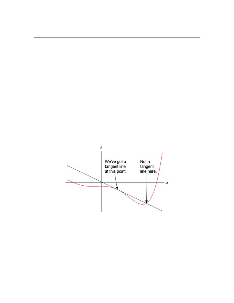
into this problem it would probably be best to define a tangent line.
A tangent line to the function f(x) at the point
x
a
=
is a line that just touches the graph of the
function at the point in question and is “parallel” (in some way) to the graph at that point. Take a
look at the graph below.
In this graph the line is a tangent line at the indicated point because it just touches the graph at
that point and is also “parallel” to the graph at that point. Likewise, at the second point shown,
the line does just touch the graph at that point, but it is not “parallel” to the graph at that point and
so it’s not a tangent line to the graph at that point.
At the second point shown (the point where the line isn’t a tangent line) we will sometimes call
the line a secant line.
We’ve used the word parallel a couple of times now and we should probably be a little careful
with it. In general, we will think of a line and a graph as being parallel at a point if they are both

Calculus I
© 2007 Paul Dawkins
5
http://tutorial.math.lamar.edu/terms.aspx
moving in the same direction at that point. So, in the first point above the graph and the line are
moving in the same direction and so we will say they are parallel at that point. At the second
point, on the other hand, the line and the graph are not moving in the same direction and so they
aren’t parallel at that point.
Okay, now that we’ve gotten the definition of a tangent line out of the way let’s move on to the
tangent line problem. That’s probably best done with an example.
Example 1
Find the tangent line to
( )
2
15 2
f x
x
=
−
at
x
= 1.
Solution
We know from algebra that to find the equation of a line we need either two points on the line or
a single point on the line and the slope of the line. Since we know that we are after a tangent line
we do have a point that is on the line. The tangent line and the graph of the function must touch
at x = 1 so the point
( )
(
)
(
)
1,
1
1,13
f
=
must be on the line.
Now we reach the problem. This is all that we know about the tangent line. In order to find the
tangent line we need either a second point or the slope of the tangent line. Since the only reason
for needing a second point is to allow us to find the slope of the tangent line let’s just concentrate
on seeing if we can determine the slope of the tangent line.
At this point in time all that we’re going to be able to do is to get an estimate for the slope of the
tangent line, but if we do it correctly we should be able to get an estimate that is in fact the actual
slope of the tangent line. We’ll do this by starting with the point that we’re after, let’s call it
(
)
1,13
P
=
. We will then pick another point that lies on the graph of the function, let’s call that
point
( )
(
)
,
Q
x f x
=
.
For the sake of argument let’s take choose
2
x
=
and so the second point will be
( )
2, 7
Q
=
.
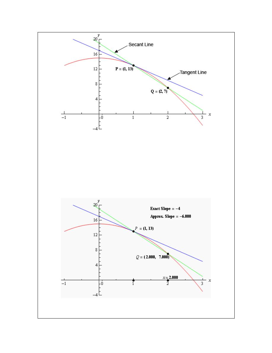
Below is a graph of the function, the tangent line and the secant line that connects P and Q.
We can see from this graph that the secant and tangent lines are somewhat similar and so the
slope of the secant line should be somewhat close to the actual slope of the tangent line. So, as an
estimate of the slope of the tangent line we can use the slope of the secant line, let’s call it
PQ
m
,
which is,
( )
( )
2
1
7 13
6
2 1
1
PQ
f
f
m
−
−
=
=
= −
−
Calculus I
© 2007 Paul Dawkins
6
http://tutorial.math.lamar.edu/terms.aspx
Now, if we weren’t too interested in accuracy we could say this is good enough and use this as an
estimate of the slope of the tangent line. However, we would like an estimate that is at least
somewhat close the actual value. So, to get a better estimate we can take an x that is closer to
1
x
=
and redo the work above to get a new estimate on the slope. We could then take a third
value of x even closer yet and get an even better estimate.
In other words, as we take Q closer and closer to P the slope of the secant line connecting Q and
P should be getting closer and closer to the slope of the tangent line. If you are viewing this on
the web, the image below shows this process.
As you can see (if you’re reading this on the web) as we moved Q in closer and closer to P the
secant lines does start to look more and more like the tangent line and so the approximate slopes
(i.e. the slopes of the secant lines) are getting closer and closer to the exact slope. Also, do not
Calculus I
© 2007 Paul Dawkins
7
http://tutorial.math.lamar.edu/terms.aspx
worry about how I got the exact or approximate slopes. We’ll be computing the approximate
slopes shortly and we’ll be able to compute the exact slope in a few sections.
In this figure we only looked at
Q
’s that were to the right of
P
, but we could have just as easily
used
Q
’s that were to the left of
P
and we would have received the same results. In fact, we
should always take a look at Q’s that are on both sides of P. In this case the same thing is
happening on both sides of P. However, we will eventually see that doesn’t have to happen.
Therefore we should always take a look at what is happening on both sides of the point in
question when doing this kind of process.
So, let’s see if we can come up with the approximate slopes I showed above, and hence an
estimation of the slope of the tangent line. In order to simplify the process a little let’s get a
formula for the slope of the line between
P
and
Q
,
PQ
m
, that will work for any x that we choose
to work with. We can get a formula by finding the slope between P and Q using the “general”
form of
( )
(
)
,
Q
x f x
=
.
( )
( )
2
2
1
15 2
13
2 2
1
1
1
PQ
f x
f
x
x
m
x
x
x
−
−
−
−
=
=
=
−
−
−
Now, let’s pick some values of
x getting closer and closer to
1
x
=
, plug in and get some
slopes.
x
PQ
m
x
PQ
m
2
-6
0
-2
1.5
-5
0.5
-3
1.1
-4.2
0.9
-3.8
1.01
-4.02
0.99
-3.98
1.001
-4.002
0.999
-3.998
1.0001 -4.0002 0.9999 -3.9998
So, if we take
x
’s to the right of 1 and move them in very close to 1 it appears that the slope of the
secant lines appears to be approaching -4. Likewise, if we take
x
’s to the left of 1 and move them
in very close to 1 the slope of the secant lines again appears to be approaching -4.
Based on this evidence it seems that the slopes of the secant lines are approaching -4 as we move
in towards
1
x
=
, so we will estimate that the slope of the tangent line is also -4. As noted above,
this is the correct value and we will be able to prove this eventually.
Now, the equation of the line that goes through
( )
(
)
,
a f a
is given by
( )
(
)
y
f a
m x a
=
+
−
Therefore, the equation of the tangent line to
( )
2
15 2
f x
x
=
−
at
x
= 1 is
(
)
13 4
1
4
17
y
x
x
=
−
− = − +

Calculus I
© 2007 Paul Dawkins
8
http://tutorial.math.lamar.edu/terms.aspx
There are a couple of important points to note about our work above. First, we looked at points
that were on both sides of
1
x
=
. In this kind of process it is important to never assume that what
is happening on one side of a point will also be happening on the other side as well. We should
always look at what is happening on both sides of the point. In this example we could sketch a
graph and from that guess that what is happening on one side will also be happening on the other,
but we will usually not have the graphs in front of us or be able to easily get them.
Next, notice that when we say we’re going to move in close to the point in question we do mean
that we’re going to move in very close and we also used more than just a couple of points. We
should never try to determine a trend based on a couple of points that aren’t really all that close to
the point in question.
The next thing to notice is really a warning more than anything. The values of
PQ
m
in this
example were fairly “nice” and it was pretty clear what value they were approaching after a
couple of computations. In most cases this will not be the case. Most values will be far
“messier” and you’ll often need quite a few computations to be able to get an estimate.
Last, we were after something that was happening at
1
x
=
and we couldn’t actually plug
1
x
=
into our formula for the slope. Despite this limitation we were able to determine some
information about what was happening at
1
x
=
simply by looking at what was happening around
1
x
=
. This is more important than you might at first realize and we will be discussing this point
in detail in later sections.
Before moving on let’s do a quick review of just what we did in the above example. We wanted
the tangent line to
( )
f x
at a point
x
a
=
. First, we know that the point
( )
(
)
,
P
a f a
=
will be
on the tangent line. Next, we’ll take a second point that is on the graph of the function, call it
( )
(
)
,
Q
x f x
=
and compute the slope of the line connecting P and Q as follows,
( )
( )
PQ
f x
f a
m
x
a
−
=
−
We then take values of x that get closer and closer to
x
a
=
(making sure to look at x’s on both
sides of
x
a
=
and use this list of values to estimate the slope of the tangent line, m.
The tangent line will then be,
( )
(
)
y
f a
m x a
=
+
−
Rates of Change
The next problem that we need to look at is the rate of change problem. This will turn out to be
one of the most important concepts that we will look at throughout this course.

Calculus I
© 2007 Paul Dawkins
9
http://tutorial.math.lamar.edu/terms.aspx
Here we are going to consider a function, f(x), that represents some quantity that varies as x
varies. For instance, maybe f(x) represents the amount of water in a holding tank after x minutes.
Or maybe f(x) is the distance traveled by a car after x hours. In both of these example we used x
to represent time. Of course x doesn’t have to represent time, but it makes for examples that are
easy to visualize.
What we want to do here is determine just how fast f(x) is changing at some point, say
x
a
=
.
This is called the instantaneous rate of change or sometimes just rate of change of f(x) at
x
a
=
.
As with the tangent line problem all that we’re going to be able to do at this point is to estimate
the rate of change. So let’s continue with the examples above and think of f(x) as something that
is changing in time and x being the time measurement. Again x doesn’t have to represent time
but it will make the explanation a little easier. While we can’t compute the instantaneous rate of
change at this point we can find the average rate of change.
To compute the average rate of change of f(x) at
x
a
=
all we need to do is to choose another
point, say x, and then the average rate of change will be,
( )
( )
( )
change in
. . .
change in
f x
A R C
x
f x
f a
x
a
=
−
=
−
Then to estimate the instantaneous rate of change at
x
a
=
all we need to do is to choose values of
x getting closer and closer to
x
a
=
(don’t forget to chose them on both sides of
x
a
=
) and
compute values of A.R.C. We can then estimate the instantaneous rate of change from that.
Let’s take a look at an example.
Example 2
Suppose that the amount of air in a balloon after t hours is given by
( )
3
2
6
35
V t
t
t
= −
+
Estimate the instantaneous rate of change of the volume after 5 hours.
Solution
Okay. The first thing that we need to do is get a formula for the average rate of change of the
volume. In this case this is,
( )
( )
3
2
3
2
5
6
35 10
6
25
. . .
5
5
5
V t
V
t
t
t
t
A R C
t
t
t
−
−
+
−
−
+
=
=
=
−
−
−
To estimate the instantaneous rate of change of the volume at
5
t
=
we just need to pick values of
t that are getting closer and closer to
5
t
=
. Here is a table of values of t and the average rate of
change for those values.
Calculus I
© 2007 Paul Dawkins
10
http://tutorial.math.lamar.edu/terms.aspx
t
A.R.C.
t
A.R.C.
6
25.0
4
7.0
5.5
19.75
4.5
10.75
5.1
15.91
4.9
14.11
5.01
15.0901
4.99
14.9101
5.001
15.009001
4.999
14.991001
5.0001 15.00090001 4.9999 14.99910001
So, from this table it looks like the average rate of change is approaching 15 and so we can
estimate that the instantaneous rate of change is 15 at this point.
So, just what does this tell us about the volume at this point? Let’s put some units on the answer
from above. This might help us to see what is happening to the volume at this point. Let’s
suppose that the units on the volume were in cm
3
. The units on the rate of change (both average
and instantaneous) are then cm
3
/hr.
We have estimated that at
5
t
=
the volume is changing at a rate of 15 cm
3
/hr. This means that
at
5
t
=
the volume is changing in such a way that, if the rate were constant, then an hour later
there would be 15 cm
3
more air in the balloon than there was at
5
t
=
.
We do need to be careful here however. In reality there probably won’t be 15 cm
3
more air in the
balloon after an hour. The rate at which the volume is changing is generally not constant and so
we can’t make any real determination as to what the volume will be in another hour. What we
can say is that the volume is increasing, since the instantaneous rate of change is positive, and if
we had rates of change for other values of t we could compare the numbers and see if the rate of
change is faster or slower at the other points.
For instance, at
4
t
=
the instantaneous rate of change is 0 cm
3
/hr and at
3
t
=
the instantaneous
rate of change is -9 cm
3
/hr. I’ll leave it to you to check these rates of change. In fact, that would
be a good exercise to see if you can build a table of values that will support my claims on these
rates of change.
Anyway, back to the example. At
4
t
=
the rate of change is zero and so at this point in time the
volume is not changing at all. That doesn’t mean that it will not change in the future. It just
means that exactly at
4
t
=
the volume isn’t changing. Likewise at
3
t
=
the volume is
decreasing since the rate of change at that point is negative. We can also say that, regardless of
the increasing/decreasing aspects of the rate of change, the volume of the balloon is changing
faster at
5
t
=
than it is at
3
t
=
since 15 is larger than 9.
We will be talking a lot more about rates of change when we get into the next chapter.

Calculus I
© 2007 Paul Dawkins
11
http://tutorial.math.lamar.edu/terms.aspx
Velocity Problem
Let’s briefly look at the velocity problem. Many calculus books will treat this as its own
problem. I however, like to think of this as a special case of the rate of change problem. In the
velocity problem we are given a position function of an object, f(t), that gives the position of an
object at time t. Then to compute the instantaneous velocity of the object we just need to recall
that the velocity is nothing more than the rate at which the position is changing.
In other words, to estimate the instantaneous velocity we would first compute the average
velocity,
( )
( )
change in position
. .
time traveled
AV
f t
f a
t
a
=
−
=
−
and then take values of t closer and closer to
t
a
=
and use these values to estimate the
instantaneous velocity.
Change of Notation
There is one last thing that we need to do in this section before we move on. The main point of
this section was to introduce us to a couple of key concepts and ideas that we will see throughout
the first portion of this course as well as get us started down the path towards limits.
Before we move into limits officially let’s go back and do a little work that will relate both (or all
three if you include velocity as a separate problem) problems to a more general concept.
First, notice that whether we wanted the tangent line, instantaneous rate of change, or
instantaneous velocity each of these came down to using exactly the same formula. Namely,
( )
( )
f x
f a
x
a
−
−
(1)
This should suggest that all three of these problems are then really the same problem. In fact this
is the case as we will see in the next chapter. We are really working the same problem in each of
these cases the only difference is the interpretation of the results.
In preparation for the next section where we will discuss this in much more detail we need to do a
quick change of notation. It’s easier to do here since we’ve already invested a fair amount of
time into these problems.
In all of these problems we wanted to determine what was happening at
x
a
=
. To do this we
chose another value of x and plugged into (1). For what we were doing here that is probably most
intuitive way of doing it. However, when we start looking at these problems as a single problem
(1) will not be the best formula to work with.

Calculus I
© 2007 Paul Dawkins
12
http://tutorial.math.lamar.edu/terms.aspx
What we’ll do instead is to first determine how far from
x
a
=
we want to move and then define
our new point based on that decision. So, if we want to move a distance of h from
x
a
=
the new
point would be
x
a
h
= +
.
As we saw in our work above it is important to take values of x that are both sides of
x
a
=
. This
way of choosing new value of x will do this for us. If h>0 we will get value of x that are to the
right of
x
a
=
and if h<0 we will get values of x that are to the left of
x
a
=
.
Now, with this new way of getting a second x, (1) will become,
( )
( )
(
)
( )
(
)
( )
f x
f a
f a
h
f a
f a
h
f a
x a
a
h a
h
−
+
−
+
−
=
=
−
+ −
(2)
On the surface it might seem that (2) is going to be an overly complicated way of dealing with
this stuff. However, as we will see it will often be easier to deal with (2) than it will be to deal
with (1).

Calculus I
© 2007 Paul Dawkins
13
http://tutorial.math.lamar.edu/terms.aspx
The Limit
In the previous
section
we looked at a couple of problems and in both problems we had a function
(slope in the tangent problem case and average rate of change in the rate of change problem) and
we wanted to know how that function was behaving at some point
x
a
=
. At this stage of the
game we no longer care where the functions came from and we no longer care if we’re going to
see them down the road again or not. All that we need to know or worry about is that we’ve got
these functions and we want to know something about them.
To answer the questions in the last section we choose values of x that got closer and closer to
x
a
=
and we plugged these into the function. We also made sure that we looked at values of x
that were on both the left and the right of
x
a
=
. Once we did this we looked at our table of
function values and saw what the function values were approaching as x got closer and closer to
x
a
=
and used this to guess the value that we were after.
This process is called taking a limit and we have some notation for this. The limit notation for
the two problems from the last section is,
2
3
2
1
5
2 2
6
25
lim
4
lim
15
1
5
x
t
x
t
t
x
t
→
→
−
−
+
= −
=
−
−
In this notation we will note that we always give the function that we’re working with and we
also give the value of x (or t) that we are moving in towards.
In this section we are going to take an intuitive approach to limits and try to get a feel for what
they are and what they can tell us about a function. With that goal in mind we are not going to
get into how we actually compute limits yet. We will instead rely on what we did in the previous
section as well as another approach to guess the value of the limits.
Both of the approaches that we are going to use in this section are designed to help us understand
just what limits are. In general we don’t typically use the methods in this section to compute
limits and in many cases can be very difficult to use to even estimate the value of a limit and/or
will give the wrong value on occasion. We will look at actually computing limits in a couple of
sections.
Let’s first start off with the following “definition” of a limit.
Definition
We say that the limit of f(x) is L as x approaches a and write this as
( )
lim
x
a
f x
L
→
=
provided we can make f(x) as close to L as we want for all x sufficiently close to a, from both
sides, without actually letting x be a.

Calculus I
© 2007 Paul Dawkins
14
http://tutorial.math.lamar.edu/terms.aspx
This is not the exact, precise definition of a limit. If you would like to see the more precise and
mathematical definition of a limit you should check out the
The Definition of a Limit
section at
the end of this chapter. The definition given above is more of a “working” definition. This
definition helps us to get an idea of just what limits are and what they can tell us about functions.
So just what does this definition mean? Well let’s suppose that we know that the limit does in
fact exist. According to our “working” definition we can then decide how close to L that we’d
like to make f(x). For sake of argument let’s suppose that we want to make f(x) no more that
0.001 away from L. This means that we want one of the following
( )
( )
( )
( )
0.001
if
is larger than L
0.001
if
is smaller than L
f x
L
f x
L
f x
f x
− <
−
<
Now according to the “working” definition this means that if we get x sufficiently close to a we
can make one of the above true. However, it actually says a little more. It actually says that
somewhere out there in the world is a value of x, say X, so that for all x’s that are closer to a than
X then one of the above statements will be true.
This is actually a fairly important idea. There are many functions out there in the world that we
can make as close to L for specific values of x that are close to a, but there will be other values of
x closer to a that give functions values that are nowhere near close to L. In order for a limit to
exist once we get f(x) as close to L as we want for some x then it will need to stay in that close to
L (or get closer) for all values of x that are closer to a. We’ll see an
example
of this later in this
section.
In somewhat simpler terms the definition says that as x gets closer and closer to x=a (from both
sides of course…) then f(x) must be getting closer and closer to L. Or, as we move in towards
x=a then f(x) must be moving in towards L.
It is important to note once again that we must look at values of x that are on both sides of x=a.
We should also note that we are not allowed to use x=a in the definition. We will often use the
information that limits give us to get some information about what is going on right at x=a, but
the limit itself is not concerned with what is actually going on at x=a. The limit is only
concerned with what is going on around the point x=a. This is an important concept about limits
that we need to keep in mind.
An alternative notation that we will occasionally use in denoting limits is
( )
as
f x
L
x
a
→
→
How do we use this definition to help us estimate limits? We do exactly what we did in the
previous
section
. We take x’s on both sides of x=a that move in closer and closer to a and we
plug these into our function. We then look to see if we can determine what number the function
values are moving in towards and use this as our estimate.
Calculus I
© 2007 Paul Dawkins
15
http://tutorial.math.lamar.edu/terms.aspx
Let’s work an example.
Example 1
Estimate the value of the following limit.
2
2
2
4
12
lim
2
x
x
x
x
x
→
+
−
−
Solution
Notice that I did say estimate the value of the limit. Again, we are not going to directly compute
limits in this section. The point of this section is to give us a better idea of how limits work and
what they can tell us about the function.
So, with that in mind we are going to work this in pretty much the same way that we did in the
last section. We will choose values of x that get closer and closer to x=2 and plug these values
into the function. Doing this gives the following table of values.
x
f(x)
x
f(x)
2.5
3.4
1.5
5.0
2.1
3.857142857 1.9
4.157894737
2.01
3.985074627 1.99
4.015075377
2.001
3.998500750 1.999
4.001500750
2.0001
3.999850007 1.9999
4.000150008
2.00001 3.999985000 1.99999 4.000015000
Note that we made sure and picked values of x that were on both sides of
2
x
=
and that
we moved in very close to
2
x
=
to make sure that any trends that we might be seeing are
in fact correct.
Also notice that we can’t actually plug in
2
x
=
into the function as this would give us a
division by zero error. This is not a problem since the limit doesn’t care what is
happening at the point in question.
From this table it appears that the function is going to 4 as x approaches 2, so
2
2
2
4
12
lim
4
2
x
x
x
x
x
→
+
−
=
−
.
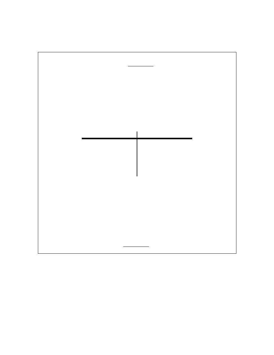
Let’s think a little bit more about what’s going on here. Let’s graph the function from the
last example. The graph of the function in the range of x’s that were interested in is
shown below.
First, notice that there is a rather large open dot at
2
x
=
. This is there to remind us that
the function (and hence the graph) doesn’t exist at
2
x
=
.
As we were plugging in values of x into the function we are in effect moving along the
graph in towards the point as
2
x
=
. This is shown in the graph by the two arrows on the
graph that are moving in towards the point.
Calculus I
© 2007 Paul Dawkins
16
http://tutorial.math.lamar.edu/terms.aspx
When we are computing limits the question that we are really asking is what y value is
our graph approaching as we move in towards x
a
= on our graph. We are NOT asking
what y value the graph takes at the point in question. In other words, we are asking what
the graph is doing around the point x
a
= . In our case we can see that as x moves in
towards 2 (from both sides) the function is approaching
4
y
=
even though the function
itself doesn’t even exist at
2
x
=
. Therefore we can say that the limit is in fact 4.
So what have we learned about limits? Limits are asking what the function is doing around
x
a
=
and are not concerned with what the function is actually doing at
x
a
=
. This is a good
thing as many of the functions that we’ll be looking at won’t even exist at
x
a
=
as we saw in our
last example.
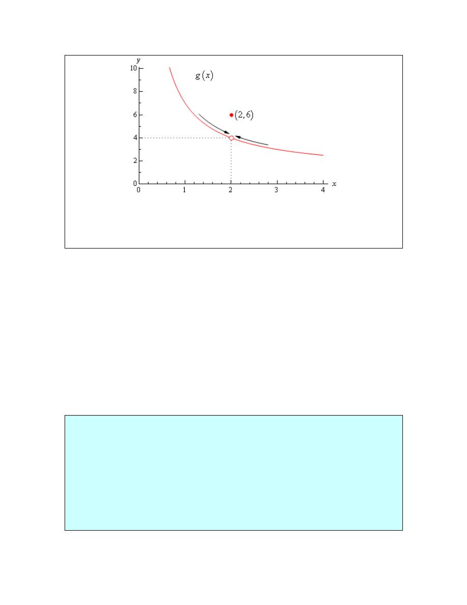
Let’s work another example to drive this point home.
Example 2
Estimate the value of the following limit.
( )
( )
2
2
2
4
12
if 2
lim
where,
2
6
if 2
x
x
x
x
g x
g x
x
x
x
→
+
−
≠
=
−
=
Solution
The first thing to note here is that this is exactly the same function as the first example with the
exception that we’ve now given it a value for
2
x
=
. So, let’s first note that
( )
2
6
g
=
As far as estimating the value of this limit goes, nothing has changed in comparison to the first
example. We could build up a table of values as we did in the first example or we could take a
quick look at the graph of the function. Either method will give us the value of the limit.
Let’s first take a look at a table of values and see what that tells us. Notice that the presence of
the value for the function at
2
x
=
will not change our choices for x. We only choose values of x
Calculus I
© 2007 Paul Dawkins
17
http://tutorial.math.lamar.edu/terms.aspx
that are getting closer to
2
x
=
but we never take
2
x
=
. In other words the table of values that
we used in the first example will be exactly the same table that we’ll use here. So, since we’ve
already got it down once there is no reason to redo it here.
From this table it is again clear that the limit is,
( )
2
lim
4
x
g x
→
=
The limit is NOT 6! Remember from the discussion after the first example that limits do not care
what the function is actually doing at the point in question. Limits are only concerned with what
is going on around the point. Since the only thing about the function that we actually changed
was its behavior at
2
x
=
this will not change the limit.
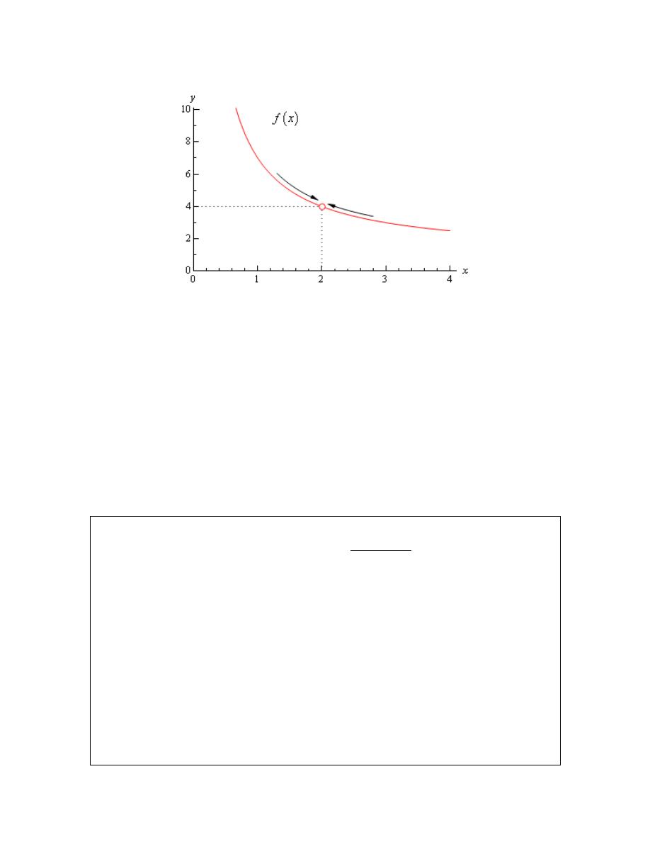
Let’s also take a quick look at this function’s graph to see if this says the same thing.
Again, we can see that as we move in towards
2
x
=
on our graph the function is still
approaching a y value of 4. Remember that we are only asking what the function is doing
around
2
x
=
and we don’t care what the function is actually doing at
2
x
=
. The graph then
also supports the conclusion that the limit is,
( )
2
lim
4
x
g x
→
=
Let’s make the point one more time just to make sure we’ve got it. Limits are not concerned with
what is going on at
x
a
=
. Limits are only concerned with what is going on around
x
a
=
. We
keep saying this, but it is a very important concept about limits that we must always keep in mind.
So, we will take every opportunity to remind ourselves of this idea.
Since limits aren’t concerned with what is actually happening at
x
a
=
we will, on occasion, see
situations like the previous example where the limit at a point and the function value at a point are
different. This won’t always happen of course. There are times where the function value and the
limit at a point are the same and we will eventually see some examples of those. It is important
however, to not get excited about things when the function and the limit do not take the same
Calculus I
© 2007 Paul Dawkins
18
http://tutorial.math.lamar.edu/terms.aspx
value at a point. It happens sometimes and so we will need to be able to deal with those cases
when they arise.
Let’s take a look another example to try and beat this idea into the ground.
Example 3
Estimate the value of the following limit.
( )
0
1 cos
lim
θ
θ
θ
→
−
Solution
First don’t get excited about the
θ
in function. It’s just a letter, just like x is a letter! It’s a Greek
letter, but it’s a letter and you will be asked to deal with Greek letters on occasion so it’s a good
idea to start getting used to them at this point.
Now, also notice that if we plug in
θ
=0 that we will get division by zero and so the function
doesn’t exist at this point. Actually, we get 0/0 at this point, but because of the division by zero
this function does not exist at
θ
=0.
So, as we did in the first example let’s get a table of values and see what if we can guess what
value the function is heading in towards.
θ
( )
f
θ
θ
( )
f
θ
1
0.45969769
-1
-0.45969769
0.1
0.04995835
-0.1
-0.04995835
0.01
0.00499996
-0.01
-0.00499996
0.001 0.00049999 -0.001 -0.00049999
Okay, it looks like the function is moving in towards a value of zero as
θ
moves in towards 0,
from both sides of course.
Therefore, the we will guess that the limit has the value,
( )
0
1 cos
lim
0
θ
θ
θ
→
−
=
So, once again, the limit had a value even though the function didn’t exist at the point we were
interested in.
It’s now time to work a couple of more examples that will lead us into the next idea about limits
that we’re going to want to discuss.
Calculus I
© 2007 Paul Dawkins
19
http://tutorial.math.lamar.edu/terms.aspx
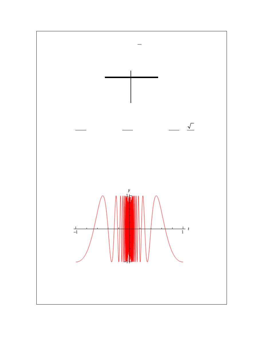
Example 4
Estimate the value of the following limit.
0
lim cos
t
t
π
→
Solution
Let’s build up a table of values and see what’s going on with our function in this case.
t
f(t)
t
f(t)
1
-1
-1
-1
0.1
1
-0.1
1
0.01
1
-0.01
1
0.001
1
-0.001
1
Now, if we were to guess the limit from this table we would guess that the limit is 1. However, if
we did make this guess we would be wrong. Consider any of the following function evaluations.
1
2
4
2
1
0
2001
2001
4001
2
f
f
f
= −
=
=
In all three of these function evaluations we evaluated the function at a number that is less that
0.001 and got three totally different numbers. Recall that the definition of the limit that we’re
working with requires that the function be approaching a single value (our guess) as t gets closer
and closer to the point in question. It doesn’t say that only some of the function values must be
getting closer to the guess. It says that all the function values must be getting closer and closer to
our guess.
To see what’s happening here a graph of the function would be convenient.
From this graph we can see that as we move in towards
0
t
=
the function starts oscillating
wildly and in fact the oscillations increases in speed the closer to
0
t
=
that we get. Recall from
our definition of the limit that in order for a limit to exist the function must be settling down in
towards a single value as we get closer to the point in question.
This function clearly does not settle in towards a single number and so this limit does not exist!
Calculus I
© 2007 Paul Dawkins
20
http://tutorial.math.lamar.edu/terms.aspx
This last example points out the drawback of just picking values of x using a table of function
values to estimate the value of a limit. The values of x that we chose in the previous example
were valid and in fact were probably values that many would have picked. In fact they were
exactly the same values we used in the problem before this one and they worked in that problem!
When using a table of values there will always be the possibility that we aren’t choosing the
correct values and that we will guess incorrectly for our limit. This is something that we should
always keep in mind when doing this to guess the value of limits. In fact, this is such a problem
that after this section we will never use a table of values to guess the value of a limit again.
This last example also has shown us that limits do not have to exist. To this point we’ve only
seen limits that have existed, but that just doesn’t always have to be the case.
Let’s take a look at one more example in this section.
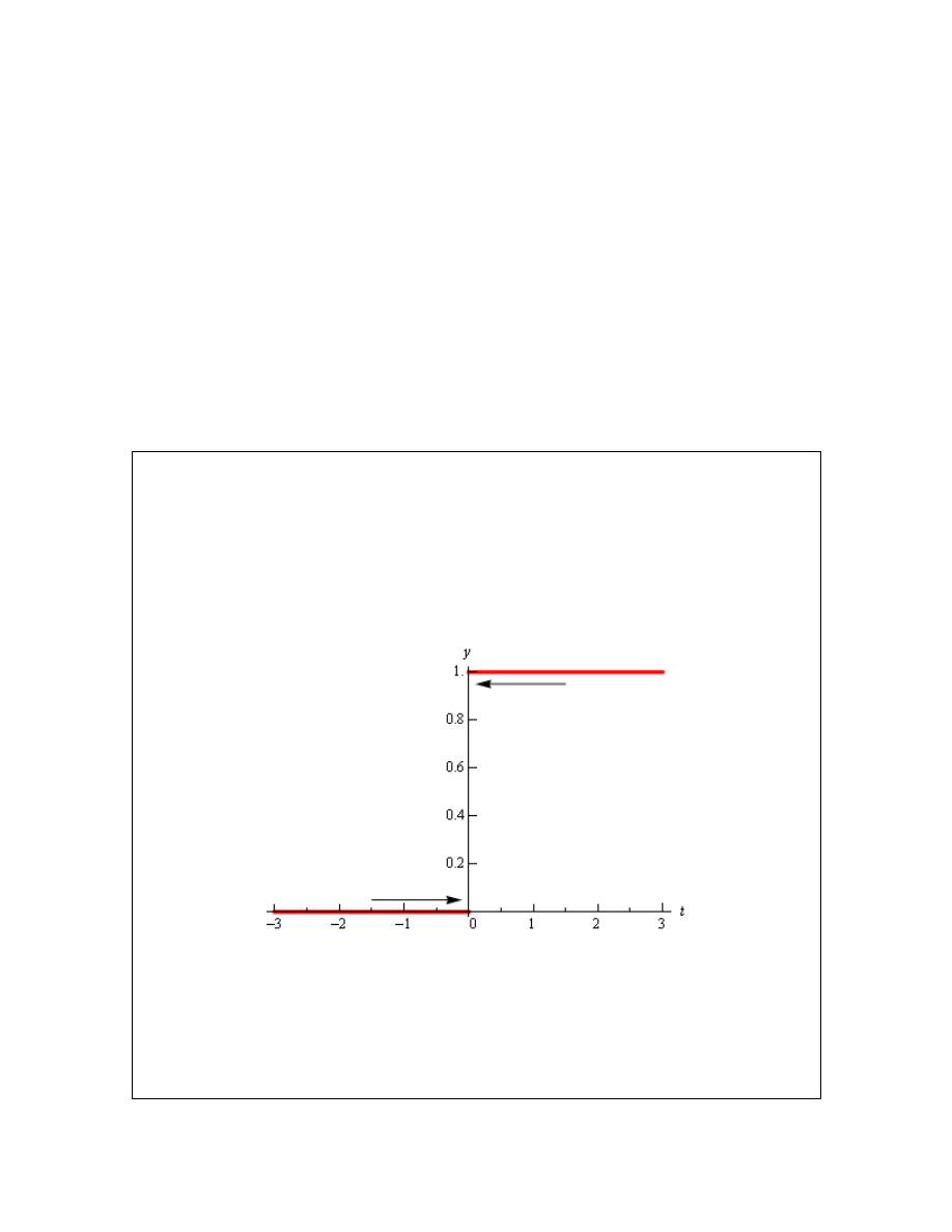
Example 5
Estimate the value of the following limit.
( )
( )
0
0
if 0
lim
where,
1
if 0
t
t
H t
H t
t
→
<
=
≥
Solution
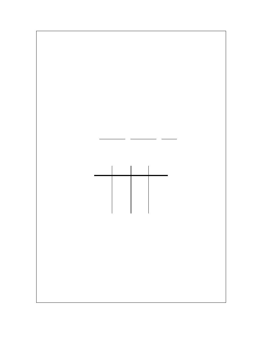
This function is often called either the Heaviside or step function. We could use a table of values
to estimate the limit, but it’s probably just as quick in this case to use the graph so let’s do that.
Below is the graph of this function.
We can see from the graph that if we approach
0
t
=
from the right side the function is moving in
towards a y value of 1. Well actually it’s just staying at 1, but in the terminology that we’ve been
using in this section it’s moving in towards 1…
Also, if we move in towards
0
t
=
from the left the function is moving in towards a y value of 0.
According to our definition of the limit the function needs to move in towards a single value as

Calculus I
© 2007 Paul Dawkins
21
http://tutorial.math.lamar.edu/terms.aspx
we move in towards
t
a
=
(from both sides). This isn’t happening in this case and so in this
example we will also say that the limit doesn’t exist.
Note that the limit in this example is a little different from the previous example. In the previous
example the function did not settle down to a single number as we moved in towards
0
t
=
. In
this example however, the function does settle down to a single number as
0
t
=
on either side.
The problem is that the number is different on each side of
0
t
=
. This is an idea that we’ll look
at in a little more detail in the next section.
Let’s summarize what we (hopefully) learned in this section. In the first three examples we saw
that limits do not care what the function is actually doing at the point in question. They only are
concerned with what is happening around the point. In fact, we can have limits at
x
a
=
even if
the function itself does not exist at that point. Likewise, even if a function exists at a point there
is no reason (at this point) to think that the limit will have the same value as the function at that
point. Sometimes the limit and the function will have the same value at a point and other times
they won’t have the same value.
Next, in the third and fourth examples we saw the main reason for not using a table of values to
guess the value of a limit. In those examples we used exactly the same set of values, however
they only worked in one of the examples. Using tables of values to guess the value of limits is
simply not a good way to get the value of a limit. This is the only section in which we will do
this. Tables of values should always be your last choice in finding values of limits.
The last two examples showed us that not all limits will in fact exist. We should not get locked
into the idea that limits will always exist. In most calculus courses we work with limits that
almost always exist and so it’s easy to start thinking that limits always exist. Limits don’t always
exist and so don’t get into the habit of assuming that they will.
Finally, we saw in the fourth example that the only way to deal with the limit was to graph the
function. Sometimes this is the only way, however this example also illustrated the drawback of
using graphs. In order to use a graph to guess the value of the limit you need to be able to
actually sketch the graph. For many functions this is not that easy to do.
There is another drawback in using graphs. Even if you actually have the graph it’s only going to
be useful if the y value is approaching an integer. If the y value is approaching say
15
123
−
there is
no way that you’re going to be able to guess that value from the graph and we are usually going
to want exact values for our limits.
So while graphs of functions can, on occasion, make your life easier in guessing values of limits
they are again probably not the best way to get values of limits. They are only going to be useful
if you can get your hands on it and the value of the limit is a “nice” number.

Calculus I
© 2007 Paul Dawkins
22
http://tutorial.math.lamar.edu/terms.aspx
The natural question then is why did we even talk about using tables and/or graphs to estimate
limits if they aren’t the best way. There were a couple of reasons.
First, they can help us get a better understanding of what limits are and what they can tell us. If
we don’t do at least a couple of limits in this way we might not get all that good of an idea on just
what limits are.
The second reason for doing limits in this way is to point out their drawback so that we aren’t
tempted to use them all the time!
We will eventually talk about how we really do limits. However, there is one more topic that we
need to discuss before doing that. Since this section has already gone on for a while we will talk
about this in the next section.

Calculus I
© 2007 Paul Dawkins
23
http://tutorial.math.lamar.edu/terms.aspx
One-Sided Limits
In the final two examples in the previous
section
we saw two limits that did not exist. However,
the reason for each of the limits not existing was different for each of the examples.
We saw that
0
lim cos
t
t
π
→
did not exist because the function did not settle down to a single value as t approached
0
t
=
.
The closer to
0
t
=
we moved the more wildly the function oscillated and in order for a limit to
exist the function must settle down to a single value.
However we saw that
( )
( )
0
0
if 0
lim
where,
1
if 0
t
t
H t
H t
t
→
<
=
≥
did not exist not because the function didn’t settle down to a single number as we moved in
towards
0
t
=
, but instead because it settled into two different numbers depending on which side
of
0
t
=
we were on.
In this case the function was a very well behaved function, unlike the first function. The only
problem was that, as we approached
0
t
=
, the function was moving in towards different numbers
on each side. We would like a way to differentiate between these two examples.
We do this with one-sided limits. As the name implies, with one-sided limits we will only be
looking at one side of the point in question. Here are the definitions for the two one sided limits.
Right-handed limit
We say
( )
lim
x
a
f x
L
+
→
=
provided we can make f(x) as close to L as we want for all x sufficiently close to a and x>a
without actually letting x be a.
Left-handed limit
We say
( )
lim
x
a
f x
L
−
→
=
provided we can make f(x) as close to L as we want for all x sufficiently close to a and x<a
without actually letting x be a.
Note that the change in notation is very minor and in fact might be missed if you aren’t paying
attention. The only difference is the bit that is under the “lim” part of the limit. For the right-
handed limit we now have
x
a
+
→
(note the “+”) which means that we know will only look at
Calculus I
© 2007 Paul Dawkins
24
http://tutorial.math.lamar.edu/terms.aspx
x>a. Likewise for the left-handed limit we have
x
a
−
→
(note the “-”) which means that we will
only be looking at x<a.
Also, note that as with the “normal” limit (i.e. the limits from the previous section) we still need
the function to settle down to a single number in order for the limit to exist. The only difference
this time is that the function only needs to settle down to a single number on either the right side
of
x
a
=
or the left side of
x
a
=
depending on the one-sided limit we’re dealing with.
So when we are looking at limits it’s now important to pay very close attention to see whether we
are doing a normal limit or one of the one-sided limits. Let’s now take a look at the some of the
problems from the last section and look at one-sided limits instead of the normal limit.
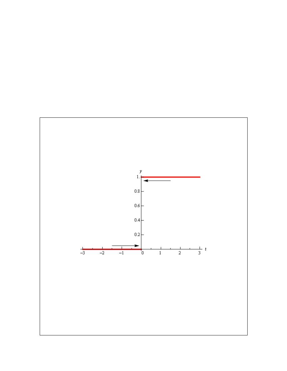
Example 1
Estimate the value of the following limits.
( )
( )
( )
0
0
0
if 0
lim
and
lim
where,
1
if 0
t
t
t
H t
H t
H t
t
+
−
→
→
<
=
≥
Solution
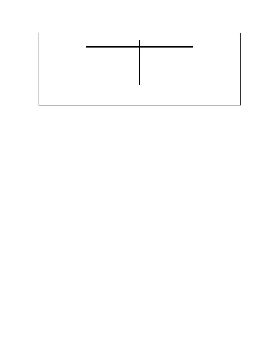
To remind us what this function looks like here’s the graph.
So, we can see that if we stay to the right of
0
t
=
(i.e.
0
t
>
) then the function is moving in
towards a value of 1 as we get closer and closer to
0
t
=
, but staying to the right. We can
therefore say that the right-handed limit is,
( )
0
lim
1
t
H t
+
→
=
Likewise, if we stay to the left of
0
t
=
(i.e
0
t
<
) the function is moving in towards a value of 0
as we get closer and closer to
0
t
=
, but staying to the left. Therefore the left-handed limit is,
( )
0
lim
0
t
H t
−
→
=
In this example we do get one-sided limits even though the normal limit itself doesn’t exist.
Calculus I
© 2007 Paul Dawkins
25
http://tutorial.math.lamar.edu/terms.aspx
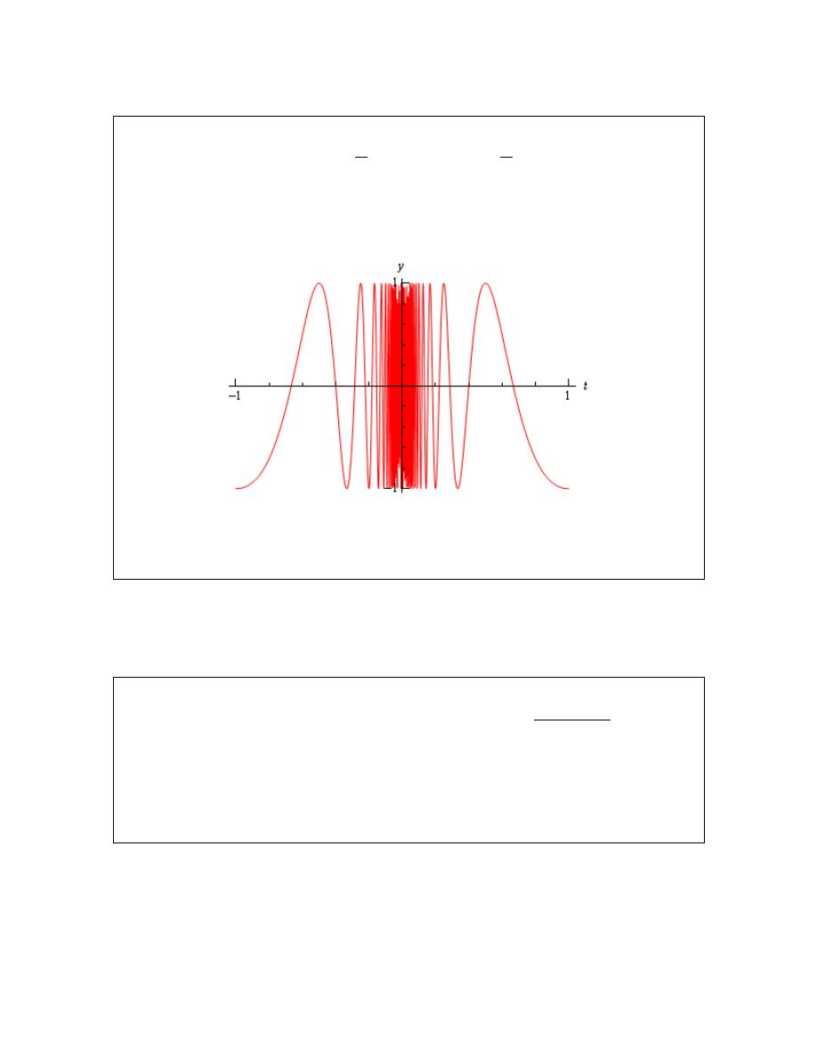
Example 2
Estimate the value of the following limits.
0
0
lim cos
lim cos
t
t
t
t
π
π
+
−
→
→
Solution
From the graph of this function shown below,
we can see that both of the one-sided limits suffer the same problem that the normal limit did in
the previous section. The function does not settle down to a single number on either side of
0
t
=
. Therefore, neither the left-handed nor the right-handed limit will exist in this case.
So, one-sided limits don’t have to exist just as normal limits aren’t guaranteed to exist.
Let’s take a look at another example from the previous section.
Example 3
Estimate the value of the following limits.
( )
( )
( )
2
2
2
2
4
12
if 2
lim
and
lim
where,
2
6
if 2
x
x
x
x
x
g x
g x
g x
x
x
x
+
−
→
→
+
−
≠
=
−
=
Solution
So as we’ve done with the previous two examples, let’s remind ourselves of the graph of this
function.
Calculus I
© 2007 Paul Dawkins
26
http://tutorial.math.lamar.edu/terms.aspx
In this case regardless of which side of
2
x
=
we are on the function is always approaching a
value of 4 and so we get,
( )
( )
2
2
lim
4
lim
4
x
x
g x
g x
+
−
→
→
=
=
Note that one-sided limits do not care about what’s happening at the point any more than normal
limits do. They are still only concerned with what is going on around the point. The only real
difference between one-sided limits and normal limits is the range of x’s that we look at when
determining the value of the limit.
Now let’s take a look at the first and last example in this section to get a very nice fact about the
relationship between one-sided limits and normal limits. In the last example the one-sided limits
as well as the normal limit existed and all three had a value of 4. In the first example the two
one-sided limits both existed, but did not have the same value and the normal limit did not exist.
The relationship between one-sided limits and normal limits can be summarized by the following
fact.
Fact
Given a function f(x) if,
( )
( )
lim
lim
x
a
x
a
f x
f x
L
+
−
→
→
=
=
then the normal limit will exist and
( )
lim
x
a
f x
L
→
=
Likewise, if
( )
lim
x
a
f x
L
→
=
then,
( )
( )
lim
lim
x
a
x
a
f x
f x
L
+
−
→
→
=
=
Calculus I
© 2007 Paul Dawkins
27
http://tutorial.math.lamar.edu/terms.aspx
This fact can be turned around to also say that if the two one-sided limits have different values,
i.e.,
( )
( )
lim
lim
x
a
x
a
f x
f x
+
−
→
→
≠
then the normal limit will not exist.
This should make some sense. If the normal limit did exist then by the fact the two one-sided
limits would have to exist and have the same value by the above fact. So, if the two one-sided
limits have different values (or don’t even exist) then the normal limit simply can’t exist.
Let’s take a look at one more example to make sure that we’ve got all the ideas about limits down
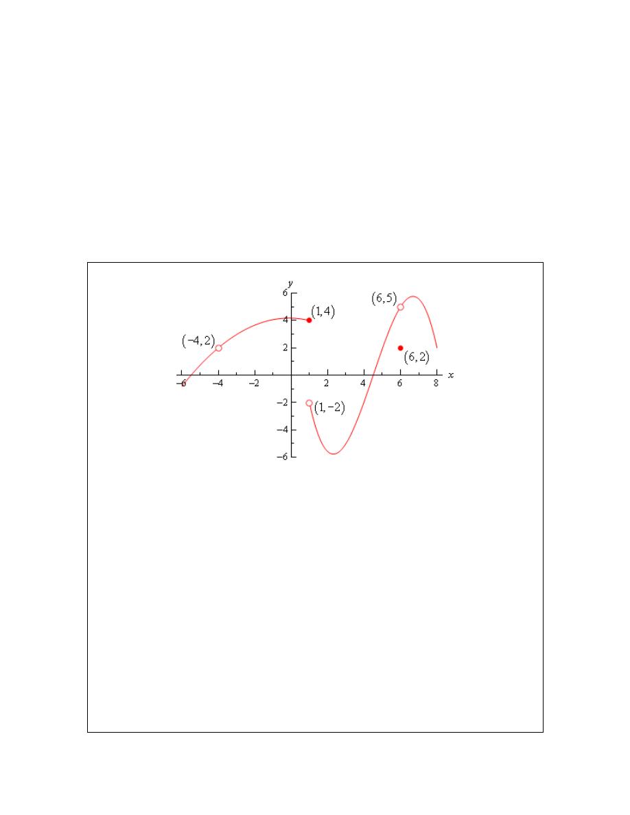
that we’ve looked at in the last couple of sections.
Example 4
Given the following graph,
compute each of the following.
(a)
( 4)
f
−
(b)
( )
4
lim
x
f x
−
→−
(c)
( )
4
lim
x
f x
+
→−
(d)
( )
4
lim
x
f x
→−
(e)
( )
1
f
(f)
( )
1
lim
x
f x
−
→
(g)
( )
1
lim
x
f x
+
→
(h)
( )
1
lim
x
f x
→
(i)
( )
6
f
(j)
( )
6
lim
x
f x
−
→
(k)
( )
6
lim
x
f x
+
→
(l)
( )
6
lim
x
f x
→
Solution
(a)
( 4)
f
−
doesn’t exist. There is no closed dot for this value of x and so the function doesn’t
exist at this point.
(b)
( )
4
lim
2
x
f x
−
→−
=
The function is approaching a value of 2 as x moves in towards -4 from the
left.
(c)
( )
4
lim
2
x
f x
+
→−
=
The function is approaching a value of 2 as x moves in towards -4 from the
right.

Calculus I
© 2007 Paul Dawkins
28
http://tutorial.math.lamar.edu/terms.aspx
(d)
( )
4
lim
2
x
f x
→−
=
We can do this one of two ways. Either we can use the fact here and notice
that the two one-sided limits are the same and so the normal limit must exist and have the same
value as the one-sided limits or just get the answer from the graph.
Also recall that a limit can exist at a point even if the function doesn’t exist at that point.
(e)
( )
1
4
f
=
. The function will take on the y value where the closed dot is.
(f)
( )
1
lim
4
x
f x
−
→
=
The function is approaching a value of 4 as x moves in towards 1 from the left.
(g)
( )
1
lim
2
x
f x
+
→
= −
The function is approaching a value of -2 as x moves in towards 1 from the
right. Remember that the limit does NOT care about what the function is actually doing at the
point, it only cares about what the function is doing around the point. In this case, always staying
to the right of
1
x
=
, the function is approaching a value of -2 and so the limit is -2. The limit is
not 4, as that is value of the function at the point and again the limit doesn’t care about that!
(h)
( )
1
lim
x
f x
→
doesn’t exist. The two one-sided limits both exist, however they are different and
so the normal limit doesn’t exist.
(i)
( )
6
2
f
=
. The function will take on the y value where the closed dot is.
(j)
( )
6
lim
5
x
f x
−
→
=
The function is approaching a value of 5 as x moves in towards 6 from the left.
(k)
( )
6
lim
5
x
f x
+
→
=
The function is approaching a value of 5 as x moves in towards 6 from the
right.
(l)
( )
6
lim
5
x
f x
→
=
Again, we can use either the graph or the fact to get this. Also, once more
remember that the limit doesn’t care what is happening at the point and so it’s possible for the
limit to have a different value than the function at a point. When dealing with limits we’ve
always got to remember that limits simply do not care about what the function is doing at the
point in question. Limits are only concerned with what the function is doing around the point.
Hopefully over the last couple of sections you’ve gotten an idea on how limits work and what
they can tell us about functions. Some of these ideas will be important in later sections so it’s
important that you have a good grasp on them.

Calculus I
© 2007 Paul Dawkins
29
http://tutorial.math.lamar.edu/terms.aspx
Limit Properties
The time has almost come for us to actually compute some limits. However, before we do that
we will need some properties of limits that will make our life somewhat easier. So, let’s take a
look at those first. The proof of some of these properties can be found in the
Proof of Various
Limit Properties
section of the Extras chapter.
Properties
First we will assume that
( )
lim
x
a
f x
→
and
( )
lim
x
a
g x
→
exist and that c is any constant. Then,
1.
( )
( )
lim
lim
x
a
x
a
cf x
c
f x
→
→
=
In other words we can “factor” a multiplicative constant out of a limit.
2.
( )
( )
( )
( )
lim
lim
lim
x
a
x
a
x
a
f x
g x
f x
g x
→
→
→
±
=
±
So to take the limit of a sum or difference all we need to do is take the limit of the
individual parts and then put them back together with the appropriate sign. This is also
not limited to two functions. This fact will work no matter how many functions we’ve
got separated by “+” or “-”.
3.
( ) ( )
( )
( )
lim
lim
lim
x
a
x
a
x
a
f x g x
f x
g x
→
→
→
=
We take the limits of products in the same way that we can take the limit of sums or
differences. Just take the limit of the pieces and then put them back together. Also, as
with sums or differences, this fact is not limited to just two functions.
4.
( )
( )
( )
( )
( )
lim
lim
,
provided lim
0
lim
x
a
x
a
x
a
x
a
f x
f x
g x
g x
g x
→
→
→
→
=
≠
As noted in the statement we only need to worry about the limit in the denominator being
zero when we do the limit of a quotient. If it were zero we would end up with a division
by zero error and we need to avoid that.
5.
( )
( )
lim
lim
,
where is any real number
n
n
x
a
x
a
f x
f x
n
→
→
=
In this property n can be any real number (positive, negative, integer, fraction, irrational,
zero, etc.). In the case that n is an integer this rule can be thought of as an extended case
of 3.
For example consider the case of n = 2.
Calculus I
© 2007 Paul Dawkins
30
http://tutorial.math.lamar.edu/terms.aspx
( )
( ) ( )
( )
( )
( )
2
2
lim
lim
lim
lim
using property 3
lim
x
a
x
a
x
a
x
a
x
a
f x
f x f x
f x
f x
f x
→
→
→
→
→
=
=
=
The same can be done for any integer n.
6.
( )
( )
lim
lim
n
n
x
a
x
a
f x
f x
→
→
=
This is just a special case of the previous example.
( )
( )
( )
( )
1
1
lim
lim
lim
lim
n
n
x
a
x
a
n
x
a
n
x
a
f x
f x
f x
f x
→
→
→
→
=
=
=
7.
lim
,
is any real number
x
a
c
c
c
→
=
In other words, the limit of a constant is just the constant. You should be able to
convince yourself of this by drawing the graph of
( )
f x
c
=
.
8.
lim
x
a
x
a
→
=
As with the last one you should be able to convince yourself of this by drawing the graph
of
( )
f x
x
=
.
9.
lim
n
n
x
a
x
a
→
=
This is really just a special case of property 5 using
( )
f x
x
=
.
Note that all these properties also hold for the two one-sided limits as well we just didn’t write
them down with one sided limits to save on space.
Let’s compute a limit or two using these properties. The next couple of examples will lead us to
some truly useful facts about limits that we will use on a continual basis.
Example 1
Compute the value of the following limit.
(
)
2
2
lim 3
5
9
x
x
x
→−
+
−
Solution
This first time through we will use only the properties above to compute the limit.

Calculus I
© 2007 Paul Dawkins
31
http://tutorial.math.lamar.edu/terms.aspx
First we will use property 2 to break up the limit into three separate limits. We will then use
property 1 to bring the constants out of the first two limits. Doing this gives us,
(
)
2
2
2
2
2
2
2
2
2
2
lim 3
5
9
lim 3
lim 5
lim 9
3 lim
5 lim
lim 9
x
x
x
x
x
x
x
x
x
x
x
x
x
→−
→−
→−
→−
→−
→−
→−
+
−
=
+
−
=
+
−
We can now use properties 7 through 9 to actually compute the limit.
(
)
( )
( )
2
2
2
2
2
2
2
lim 3
5
9
3 lim
5 lim
lim 9
3
2
5
2
9
7
x
x
x
x
x
x
x
x
→−
→−
→−
→−
+
−
=
+
−
= −
+ − −
= −
Now, let’s notice that if we had defined
( )
2
3
5
9
p x
x
x
=
+
−
then the proceeding example would have been,
( )
(
)
( )
( )
( )
2
2
2
2
lim
lim 3
5
9
3
2
5
2
9
7
2
x
x
p x
x
x
p
→−
→−
=
+
−
= −
+ − −
= −
=
−
In other words, in this case we see that the limit is the same value that we’d get by just evaluating
the function at the point in question. This seems to violate one of the main concepts about limits
that we’ve seen to this point.
In the previous two sections we made a big deal about the fact that limits do not care about what
is happening at the point in question. They only care about what is happening around the point.
So how does the previous example fit into this since it appears to violate this main idea about
limits?
Despite appearances the limit still doesn’t care about what the function is doing at
2
x
= −
. In
this case the function that we’ve got is simply “nice enough” so that what is happening around the
point is exactly the same as what is happening at the point.
Eventually
we will formalize up just
what is meant by “nice enough”. At this point let’s not worry too much about what “nice
enough” is. Let’s just take advantage of the fact that some functions will be “nice enough”,
whatever that means.
The function in the last example was a polynomial. It turns out that all polynomials are “nice
enough” so that what is happening around the point is exactly the same as what is happening at
the point. This leads to the following fact.

Calculus I
© 2007 Paul Dawkins
32
http://tutorial.math.lamar.edu/terms.aspx
Fact
If p(x) is a polynomial then,
( )
( )
lim
x
a
p x
p a
→
=
By the end of this section we will generalize this out considerably to most of the functions that
we’ll be seeing throughout this course.
Let’s take a look at another example.
Example 2
Evaluate the following limit.
2
4
3
1
6 3
10
lim
2
7
1
z
z
z
z
z
→
−
+
−
+
+
Solution
First notice that we can use property 4) to write the limit as,
2
2
1
4
3
4
3
1
1
lim 6 3
10
6 3
10
lim
2
7
1
lim 2
7
1
z
z
z
z
z
z
z
z
z
z
z
→
→
→
−
+
−
+
=
−
+
+
−
+
+
Well, actually we should be a little careful. We can do that provided the limit of the denominator
isn’t zero. As we will see however, it isn’t in this case so we’re okay.
Now, both the numerator and denominator are polynomials so we can use the fact above to
compute the limits of the numerator and the denominator and hence the limit itself.
( )
( )
( )
( )
2
2
4
3
4
3
1
6 3 1
10 1
6 3
10
lim
2
7
1
2 1
7 1
1
13
6
z
z
z
z
z
→
−
+
−
+
=
−
+
+
−
+
+
=
Notice that the limit of the denominator wasn’t zero and so our use of property 4 was legitimate.
Notice in this last example that again all we really did was evaluate the function at the point in
question. So it appears that there is a fairly large class of functions for which this can be done.
Let’s generalize the fact from above a little.
Fact
Provided f(x) is “nice enough” we have,
( )
( )
( )
( )
( )
( )
lim
lim
lim
x
a
x
a
x
a
f x
f a
f x
f a
f x
f a
−
+
→
→
→
=
=
=
Calculus I
© 2007 Paul Dawkins
33
http://tutorial.math.lamar.edu/terms.aspx
Again, we will formalize up just what we mean by “nice enough”
eventually
. At this point all we
want to do is worry about which functions are “nice enough”. Some functions are “nice enough”
for all x while others will only be “nice enough” for certain values of x. It will all depend on the
function.
As noted in the statement, this fact also holds for the two one-sided limits as well as the normal
limit.
Here is a list of some of the more common functions that are “nice enough”.
• Polynomials are nice enough for all x’s.
• If
( )
( )
( )
p x
f x
q x
=
then f(x) will be nice enough provided both p(x) and q(x) are nice
enough and if we don’t get division by zero at the point we’re evaluating at.
•
( )
( )
cos
, sin
x
x
are nice enough for all x’s
•
( )
( )
sec
, tan
x
x
are nice enough provided
5
3
3
5
,
,
,
,
,
,
2
2
2
2
2
x
π
π π π π
≠
−
−
In other
words secant and tangent are nice enough everywhere cosine isn’t zero. To see why
recall that these are both really rational functions and that cosine is in the denominator of
both then go back up and look at the second bullet above.
•
( )
( )
csc
, cot
x
x
are nice enough provided
, 2 ,
, 0,
, 2 ,
x
π
π
π π
≠
−
−
In other
words cosecant and cotangent are nice enough everywhere sine isn’t zero.
•
n
x
is nice enough for all x if n is odd.
•
n
x
is nice enough for
0
x
≥
if n is even. Here we require
0
x
≥
to avoid having to
deal with complex values.
•
,
x
x
a
e
are nice enough for all x’s.
•
log
, ln
b
x
x
are nice enough for x>0. Remember we can only plug positive numbers
into logarithms and not zero or negative numbers.
• Any sum, difference or product of the above functions will also be nice enough.
Quotients will be nice enough provided we don’t get division by zero upon evaluating the
limit.
The last bullet is important. This means that for any combination of these functions all we need
to do is evaluate the function at the point in question, making sure that none of the restrictions are
violated. This means that we can now do a large number of limits.
Example 3
Evaluate the following limit.
( )
( ) ( )
5
3
lim
sin
cos
1 ln
x
x
x
x
x
x
→
−
+
+
+
e
Solution
This is a combination of several of the functions listed above and none of the restrictions are
violated so all we need to do is plug in
3
x
=
into the function to get the limit.

Calculus I
© 2007 Paul Dawkins
34
http://tutorial.math.lamar.edu/terms.aspx
( )
( ) ( )
( )
( ) ( )
3
5
5
3
lim
sin
cos
3
sin 3 cos 3
1 ln
1 ln 3
8.185427271
x
x
x
x
x
x
→
−
+
+
= −
+
+
+
+
=
e
e
Not a very pretty answer, but we can now do the limit.

Calculus I
© 2007 Paul Dawkins
35
http://tutorial.math.lamar.edu/terms.aspx
Computing Limits
In the previous
section
we saw that there is a large class of function that allows us to use
( )
( )
lim
x
a
f x
f a
→
=
to compute limits. However, there are also many limits for which this won’t work easily. The
purpose of this section is to develop techniques for dealing with some of these limits that will not
allow us to just use this fact.
Let’s first got back and take a look at one of the first limits that we looked at and compute its
exact value and verify our guess for the limit.
Example 1
Evaluate the following limit.
2
2
2
4
12
lim
2
x
x
x
x
x
→
+
−
−
Solution
First let’s notice that if we try to plug in
2
x
=
we get,
2
2
2
4
12
0
lim
2
0
x
x
x
x
x
→
+
−
=
−
So, we can’t just plug in
2
x
=
to evaluate the limit. So, we’re going to have to do something
else.
The first thing that we should always do when evaluating limits is to simplify the function as
much as possible. In this case that means factoring both the numerator and denominator. Doing
this gives,
(
)(
)
(
)
2
2
2
2
2
2
6
4
12
lim
lim
2
2
6
lim
x
x
x
x
x
x
x
x
x
x x
x
x
→
→
→
−
+
+
−
=
−
−
+
=
So, upon factoring we saw that we could cancel an
2
x
−
from both the numerator and the
denominator. Upon doing this we now have a new rational expression that we can plug
2
x
=
into because we lost the division by zero problem. Therefore, the limit is,
2
2
2
2
4
12
6
8
lim
lim
4
2
2
x
x
x
x
x
x
x
x
→
→
+
−
+
=
= =
−
Note that this is in fact what we guessed the limit to be.
On a side note, the 0/0 we initially got in the previous example is called an indeterminate form.
This means that we don’t really know what it will be until we do some more work. Typically
zero in the denominator means it’s undefined. However that will only be true if the numerator
isn’t also zero. Also, zero in the numerator usually means that the fraction is zero, unless the

Calculus I
© 2007 Paul Dawkins
36
http://tutorial.math.lamar.edu/terms.aspx
denominator is also zero. Likewise anything divided by itself is 1, unless we’re talking about
zero.
So, there are really three competing “rules” here and it’s not clear which one will win out. It’s
also possible that none of them will win out and we will get something totally different from
undefined, zero, or one. We might, for instance, get a value of 4 out of this, to pick a number
completely at random.
There are many more kinds of indeterminate forms and we will be discussing indeterminate forms
at length in the next chapter.
Let’s take a look at a couple of more examples.
Example 2
Evaluate the following limit.
(
)
2
0
2
3
18
lim
h
h
h
→
− +
−
Solution
In this case we also get 0/0 and factoring is not really an option. However, there is still some
simplification that we can do.
(
)
(
)
2
2
0
0
2
0
2
0
2 9 6
18
2
3
18
lim
lim
18 12
2
18
lim
12
2
lim
h
h
h
h
h
h
h
h
h
h
h
h
h
h
h
→
→
→
→
−
+
−
− +
−
=
−
+
−
=
−
+
=
So, upon multiplying out the first term we get a little cancellation and now notice that we can
factor an h out of both terms in the numerator which will cancel against the h in the denominator
and the division by zero problem goes away and we can then evaluate the limit.
(
)
(
)
2
2
0
0
0
0
2
3
18
12
2
lim
lim
12 2
lim
lim
12 2
12
h
h
h
h
h
h
h
h
h
h
h
h
h
→
→
→
→
− +
−
−
+
=
− +
=
=
− +
= −
Example 3
Evaluate the following limit.
4
3
4
lim
4
t
t
t
t
→
−
+
−
Solution
This limit is going to be a little more work than the previous two. Once again however note that
we get the indeterminate form 0/0 if we try to just evaluate the limit. Also note that neither of the
Calculus I
© 2007 Paul Dawkins
37
http://tutorial.math.lamar.edu/terms.aspx
two examples will be of any help here, at least initially. We can’t factor and we can’t just
multiply something out to get the function to simplify.
When there is a square root in the numerator or denominator we can try to rationalize and see if
that helps. Recall that rationalizing makes use of the fact that
(
)(
)
2
2
a b
a b
a
b
+
−
=
−
So, if either the first and/or the second term have a square root in them the rationalizing will
eliminate the root(s). This might help in evaluating the limit.
Let’s try rationalizing the numerator in this case.
(
)
(
)
(
)
(
)
4
4
3
4
3
4
3
4
lim
lim
4
4
3
4
t
t
t
t
t
t
t
t
t
t
t
t
→
→
−
+
+
+
−
+
=
−
−
+
+
Remember that to rationalize we just take the numerator (since that’s what we’re rationalizing),
change the sign on the second term and multiply the numerator and denominator by this new
term.
Next, we multiply the numerator out being careful to watch minus signs.
(
)
(
)
(
)
(
)
(
)
2
4
4
2
4
3
4
3
4
lim
lim
4
4
3
4
3
4
lim
4
3
4
t
t
t
t
t
t
t
t
t
t
t
t
t
t
t
t
→
→
→
−
+
−
+
=
−
−
+
+
− −
=
−
+
+
Notice that we didn’t multiply the denominator out as well. Most students come out of an
Algebra class having it beaten into their heads to always multiply this stuff out. However, in this
case multiplying out will make the problem very difficult and in the end you’ll just end up
factoring it back out anyway.
At this stage we are almost done. Notice that we can factor the numerator so let’s do that.
(
)(
)
(
)
(
)
4
4
4
1
3
4
lim
lim
4
4
3
4
t
t
t
t
t
t
t
t
t
t
→
→
−
+
−
+
=
−
−
+
+
Now all we need to do is notice that if we factor a “-1”out of the first term in the denominator we
can do some canceling. At that point the division by zero problem will go away and we can
evaluate the limit.
Calculus I
© 2007 Paul Dawkins
38
http://tutorial.math.lamar.edu/terms.aspx
(
)(
)
(
)
(
)
(
)
4
4
4
4
1
3
4
lim
lim
4
4
3
4
1
lim
3
4
5
8
t
t
t
t
t
t
t
t
t
t
t
t
t
t
→
→
→
−
+
−
+
=
−
− −
+
+
+
=
− +
+
= −
Note that if we had multiplied the denominator out we would not have been able to do this
canceling and in all likelihood would not have even seen that some canceling could have been
done.
So, we’ve taken a look at a couple of limits in which evaluation gave the indeterminate form 0/0
and we now have a couple of things to try in these cases.
Let’s take a look at another kind of problem that can arise in computing some limits involving
piecewise functions.
Example 4
Given the function,
( )
2
5 if 2
1 3
if 2
y
y
g y
y
y
+
< −
=
−
≥ −
Compute the following limits.
(a)
( )
6
lim
y
g y
→
[
Solution
]
(b)
( )
2
lim
y
g y
→−
[
Solution
]
Solution
(a)
( )
6
lim
y
g y
→
In this case there really isn’t a whole lot to do. In doing limits recall that we must always look at
what’s happening on both sides of the point in question as we move in towards it. In this case
6
y
=
is completely inside the second interval for the function and so there are values of y on
both sides of
6
y
=
that are also inside this interval. This means that we can just use the fact to
evaluate this limit.
( )
6
6
lim
lim1 3
17
y
y
g y
y
→
→
=
−
= −
[
Return to Problems
]
(b)
( )
2
lim
y
g y
→−
This part is the real point to this problem. In this case the point that we want to take the limit for
is the cutoff point for the two intervals. In other words we can’t just plug
2
y
= −
into the second

Calculus I
© 2007 Paul Dawkins
39
http://tutorial.math.lamar.edu/terms.aspx
portion because this interval does not contain values of y to the left of
2
y
= −
and we need to
know what is happening on both sides of the point.
To do this part we are going to have to remember the fact from the section on
one-sided limits
that says that if the two one-sided limits exist and are the same then the normal limit will also
exist and have the same value.
Notice that both of the one sided limits can be done here since we are only going to be looking at
one side of the point in question. So let’s do the two one-sided limits and see what we get.
( )
2
2
2
lim
lim
5
since
2 implies
2
9
y
y
g y
y
y
y
−
−
−
→−
→−
=
+
→
< −
=
( )
2
2
lim
lim 1 3
since
2 implies
2
7
y
y
g y
y
y
y
+
+
+
→−
→−
=
−
→
> −
=
So, in this case we can see that,
( )
( )
2
2
lim
9
7
lim
y
y
g y
g y
−
+
→−
→−
= ≠ =
and so since the two one sided limits aren’t the same
( )
2
lim
y
g y
→−
doesn’t exist.
[
Return to Problems
]
Note that a very simple change to the function will make the limit at
2
y
= −
exist so don’t get in
into your head that limits at these cutoff points in piecewise function don’t ever exist.
Example 5
Evaluate the following limit.
( )
( )
2
2
5 if 2
lim
where,
3 3
if 2
y
y
y
g y
g y
y
y
→−
+
< −
=
−
≥ −
Solution
The two one-sided limits this time are,
( )
2
2
2
lim
lim
5
since
2 implies
2
9
y
y
g y
y
y
y
−
−
−
→−
→−
=
+
→
< −
=
( )
2
2
lim
lim 3 3
since
2 implies
2
9
y
y
g y
y
y
y
+
−
+
→−
→−
=
−
→
> −
=
The one-sided limits are the same so we get,
( )
2
lim
9
y
g y
→−
=

Calculus I
© 2007 Paul Dawkins
40
http://tutorial.math.lamar.edu/terms.aspx
There is one more limit that we need to do. However, we will need a new fact about limits that
will help us to do this.
Fact
If
( )
( )
f x
g x
≤
for all x on [a, b] (except possibly at
x
c
=
) and
a
c
b
≤ ≤
then,
( )
( )
lim
lim
x
c
x
c
f x
g x
→
→
≤
Note that this fact should make some sense to you if we assume that both functions are nice
enough. If both of the functions are “nice enough” to use the limit evaluation
fact
then we have,
( )
( )
( )
( )
lim
lim
x
c
x
c
f x
f c
g c
g x
→
→
=
≤
=
The inequality is true because we know that c is somewhere between a and b and in that range we
also know
( )
( )
f x
g x
≤
.
Note that we don’t really need the two functions to be nice enough for the fact to be true, but it
does provide a nice way to give a quick “justification” for the fact.
Also, note that we said that we assumed that
( )
( )
f x
g x
≤
for all x on [a, b] (except possibly at
x
c
=
). Because limits do not care what is actually happening at
x
c
=
we don’t really need the
inequality to hold at that specific point. We only need it to hold around
x
c
=
since that is what
the limit is concerned about.
We can take this fact one step farther to get the following theorem.
Squeeze Theorem
Suppose that for all x on [a, b] (except possibly at
x
c
=
) we have,
( ) ( )
( )
f x
h x
g x
≤
≤
Also suppose that,
( )
( )
lim
lim
x
c
x
c
f x
g x
L
→
→
=
=
for some
a
c
b
≤ ≤
. Then,
( )
lim
x
c
h x
L
→
=
As with the previous fact we only need to know that
( ) ( )
( )
f x
h x
g x
≤
≤
is true around
x
c
=
because we are working with limits and they are only concerned with what is going on around
x
c
=
and not what is actually happening at
x
c
=
.
Now, if we again assume that all three functions are nice enough (again this isn’t required to
make the Squeeze Theorem true, it only helps with the visualization) then we can get a quick
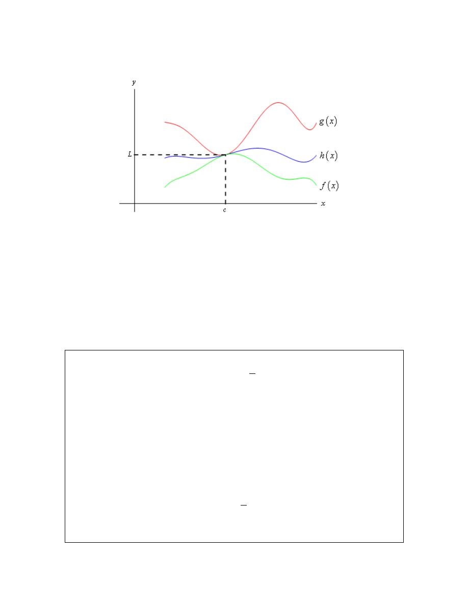
Calculus I
© 2007 Paul Dawkins
41
http://tutorial.math.lamar.edu/terms.aspx
sketch of what the Squeeze Theorem is telling us. The following figure illustrates what is
happening in this theorem.
From the figure we can see that if the limits of f(x) and g(x) are equal at
x
c
=
then the function
values must also be equal at
x
c
=
(this is where we’re using the fact that we assumed the
functions where “nice enough”, which isn’t really required for the Theorem). However, because
h(x) is “squeezed” between f(x) and g(x) at this point then h(x) must have the same value.
Therefore, the limit of h(x) at this point must also be the same.
The Squeeze theorem is also known as the Sandwich Theorem and the Pinching Theorem.
So, how do we use this theorem to help us with limits? Let’s take a look at the following
example to see the theorem in action.
Example 6
Evaluate the following limit.
2
0
1
lim
cos
x
x
x
→
Solution
In this example none of the previous examples can help us. There’s no factoring or simplifying to
do. We can’t rationalize and one-sided limits won’t work. There’s even a question as to whether
this limit will exist since we have division by zero inside the cosine at x=0.
The first thing to notice is that we know the following fact about cosine.
( )
1 cos
1
x
− ≤
≤
Our function doesn’t have just an x in the cosine, but as long as we avoid
0
x
=
we can say the
same thing for our cosine.
1
1 cos
1
x
− ≤
≤
It’s okay for us to ignore
0
x
=
here because we are taking a limit and we know that limits don’t
care about what’s actually going on at the point in question,
0
x
=
in this case.

Calculus I
© 2007 Paul Dawkins
42
http://tutorial.math.lamar.edu/terms.aspx
Now if we have the above inequality for our cosine we can just multiply everything by an x
2
and
get the following.
2
2
2
1
cos
x
x
x
x
− ≤
≤
In other words we’ve managed to squeeze the function that we were interested in between two
other functions that are very easy to deal with. So, the limits of the two outer functions are.
( )
2
2
0
0
lim
0
lim
0
x
x
x
x
→
→
=
−
=
These are the same and so by the Squeeze theorem we must also have,
2
0
1
lim
cos
0
x
x
x
→
=
We can verify this with the graph of the three functions. This is shown below.
In this section we’ve seen several tools that we can use to help us to compute limits in which we
can’t just evaluate the function at the point in question. As we will see many of the limits that
we’ll be doing in later sections will require one or more of these tools.

Calculus I
© 2007 Paul Dawkins
43
http://tutorial.math.lamar.edu/terms.aspx
Infinite Limits
In this section we will take a look at limits whose value is infinity or minus infinity. These kinds
of limit will show up fairly regularly in later sections and in other courses and so you’ll need to
be able to deal with them when you run across them.
The first thing we should probably do here is to define just what we mean when we say that a
limit has a value of infinity or minus infinity.
Definition
We say
( )
lim
x
a
f x
→
= ∞
if we can make f(x) arbitrarily large for all x sufficiently close to x=a, from both sides, without
actually letting
x
a
=
.
We say
( )
lim
x
a
f x
→
= −∞
if we can make f(x) arbitrarily large and negative for all x sufficiently close to x=a, from both
sides, without actually letting
x
a
=
.
These definitions can be appropriately modified for the one-sided limits as well. To see a more
precise and mathematical definition of this kind of limit see the
The Definition of the Limit
section at the end of this chapter.
Let’s start off with a fairly typical example illustrating infinite limits.
Example 1
Evaluate each of the following limits.
0
0
0
1
1
1
lim
lim
lim
x
x
x
x
x
x
+
−
→
→
→
Solution
So we’re going to be taking a look at a couple of one-sided limits as well as the normal limit here.
In all three cases notice that we can’t just plug in
0
x
=
. If we did we would get division by
zero. Also recall that the definitions above can be easily modified to give similar definitions for
the two one-sided limits which we’ll be needing here.
Now, there are several ways we could proceed here to get values for these limits. One way is to
plug in some points and see what value the function is approaching. In the preceding section we
said that we were no longer going to do this, but in this case it is a good way to illustrate just
what’s going on with this function.
So, here is a table of values of x’s from both the left and the right. Using these values we’ll be
able to estimate the value of the two one-sided limits and once we have that done we can use the
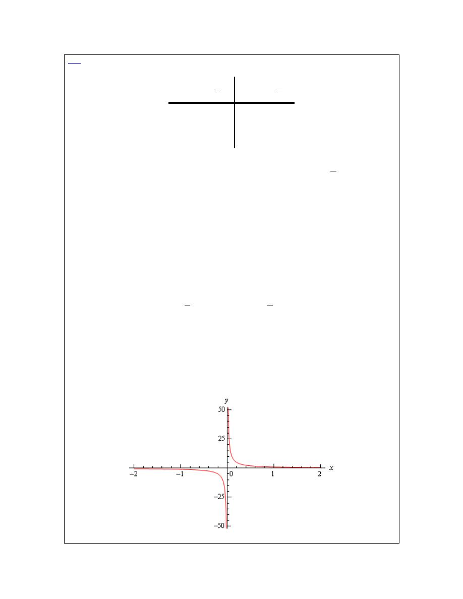
Calculus I
© 2007 Paul Dawkins
44
http://tutorial.math.lamar.edu/terms.aspx
fact
that the normal limit will exist only if the two one-sided limits exist and have the same value.
x
1
x
x
1
x
-0.1
-10
0.1
10
-0.01
-100
0.01
100
-0.001
-1000
0.001
1000
-0.0001 -10000 0.0001 10000
From this table we can see that as we make x smaller and smaller the function
1
x
gets larger and
larger and will retain the same sign that x originally had. It should make sense that this trend will
continue for any smaller value of x that we chose to use. The function is a constant (one in this
case) divided by an increasingly small number. The resulting fraction should be an increasingly
large number and as noted above the fraction will retain the same sign as x.
We can make the function as large and positive as we want for all x’s sufficiently close to zero
while staying positive (i.e. on the right). Likewise, we can make the function as large and
negative as we want for all x’s sufficiently close to zero while staying negative (i.e. on the left).
So, from our definition above it looks like we should have the following values for the two one
sided limits.
0
0
1
1
lim
lim
x
x
x
x
+
−
→
→
= ∞
= −∞
Another way to see the values of the two one sided limits here is to graph the function. Again, in
the previous section we mentioned that we won’t do this too often as most functions are not
something we can just quickly sketch out as well as the problems with accuracy in reading values
off the graph. In this case however, it’s not too hard to sketch a graph of the function and, in this
case as we’ll see accuracy is not really going to be an issue. So, here is a quick sketch of the
graph.

Calculus I
© 2007 Paul Dawkins
45
http://tutorial.math.lamar.edu/terms.aspx
So, we can see from this graph that the function does behave much as we predicted that it would
from our table values. The closer x gets to zero from the right the larger (in the positive sense)
the function gets, while the closer x gets to zero from the left the larger (in the negative sense) the
function gets.
Finally, the normal limit, in this case, will not exist since the two one-sided limits have different
values.
So, in summary here are the values of the three limits for this example.
0
0
0
1
1
1
lim
lim
lim
doesn't exist
x
x
x
x
x
x
+
−
→
→
→
= ∞
= −∞
For most of the remaining examples in this section we’ll attempt to “talk our way through” each
limit. This means that we’ll see if we can analyze what should happen to the function as we get
very close to the point in question without actually plugging in any values into the function. For
most of the following examples this kind of analysis shouldn’t be all that difficult to do. We’ll
also verify our analysis with a quick graph.
So, let’s do a couple more examples.
Example 2
Evaluate each of the following limits.
2
2
2
0
0
0
6
6
6
lim
lim
lim
x
x
x
x
x
x
+
−
→
→
→
Solution
As with the previous example let’s start off by looking at the two one-sided limits. Once we have
those we’ll be able to determine a value for the normal limit.
So, let’s take a look at the right-hand limit first and as noted above let’s see if we can figure out
what each limit will be doing without actually plugging in any values of x into the function. As
we take smaller and smaller values of x, while staying positive, squaring them will only make
them smaller (recall squaring a number between zero and one will make it smaller) and of course
it will stay positive. So we have a positive constant divided by an increasingly small positive
number. The result should then be an increasingly large positive number. It looks like we should
have the following value for the right-hand limit in this case,
2
0
6
lim
x
x
+
→
= ∞
Now, let’s take a look at the left hand limit. In this case we’re going to take smaller and smaller
values of x, while staying negative this time. When we square them they’ll get smaller, but upon
squaring the result is now positive. So, we have a positive constant divided by an increasingly
small positive number. The result, as with the right hand limit, will be an increasingly large
positive number and so the left-hand limit will be,
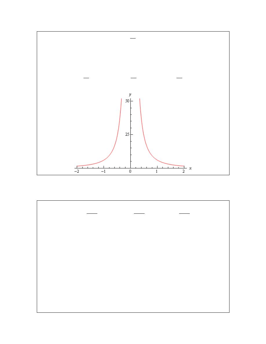
Calculus I
© 2007 Paul Dawkins
46
http://tutorial.math.lamar.edu/terms.aspx
2
0
6
lim
x
x
−
→
= ∞
Now, in this example, unlike the first one, the normal limit will exist and be infinity since the two
one-sided limits both exist and have the same value. So, in summary here are all the limits for
this example as well as a quick graph verifying the limits.
2
2
2
0
0
0
6
6
6
lim
lim
lim
x
x
x
x
x
x
+
−
→
→
→
= ∞
= ∞
= ∞
With this next example we’ll move away from just an x in the denominator, but as we’ll see in the
next couple of examples they work pretty much the same way.
Example 3
Evaluate each of the following limits.
2
2
2
4
4
4
lim
lim
lim
2
2
2
x
x
x
x
x
x
+
−
→−
→−
→−
−
−
−
+
+
+
Solution
Let’s again start with the right-hand limit. With the right hand limit we know that we have,
2
2
0
x
x
> −
⇒
+ >
Also, as x gets closer and closer to -2 then
2
x
+
will be getting closer and closer to zero, while
staying positive as noted above. So, for the right-hand limit, we’ll have a negative constant
divided by an increasingly small positive number. The result will be an increasingly large and
negative number. So, it looks like the right-hand limit will be negative infinity.
For the left hand limit we have,
2
2
0
x
x
< −
⇒
+ <
and
2
x
+
will get closer and closer to zero (and be negative) as x gets closer and closer to -2. In
this case then we’ll have a negative constant divided by an increasingly small negative number.
The result will then be an increasingly large positive number and so it looks like the left-hand
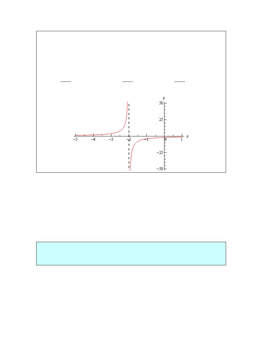
Calculus I
© 2007 Paul Dawkins
47
http://tutorial.math.lamar.edu/terms.aspx
limit will be positive infinity.
Finally, since two one sided limits are not the same the normal limit won’t exist.
Here are the official answers for this example as well as a quick graph of the function for
verification purposes.
2
2
2
4
4
4
lim
lim
lim
doesn't exist
2
2
2
x
x
x
x
x
x
+
−
→−
→−
→−
−
−
−
= −∞
= ∞
+
+
+
At this point we should briefly acknowledge the idea of vertical asymptotes. Each of the three
previous graphs have had one. Recall from an Algebra class that a vertical asymptote is a vertical
line (the dashed line at
2
x
= −
in the previous example) in which the graph will go towards
infinity and/or minus infinity on one or both sides of the line.
In an Algebra class they are a little difficult to define other than to say pretty much what we just
said. Now that we have infinite limits under our belt we can easily define a vertical asymptote as
follows,
Definition
The function f(x) will have a vertical asymptote at
x
a
=
if we have any of the following limits at
x
a
=
.
( )
( )
( )
lim
lim
lim
x
a
x
a
x
a
f x
f x
f x
−
+
→
→
→
= ± ∞
= ± ∞
= ± ∞
Note that it only requires one of the above limits for a function to have a vertical asymptote at
x
a
=
.
Using this definition we can see that the first two examples had vertical asymptotes at
0
x
=
while the third example had a vertical asymptote at
2
x
= −
.

Calculus I
© 2007 Paul Dawkins
48
http://tutorial.math.lamar.edu/terms.aspx
We aren’t really going to do a lot with vertical asymptotes here, but wanted to mention them at
this point since we’d reached a good point to do that.
Let’s now take a look at a couple more examples of infinite limits that can cause some problems
on occasion.
Example 4
Evaluate each of the following limits.
(
)
(
)
(
)
3
3
3
4
4
4
3
3
3
lim
lim
lim
4
4
4
x
x
x
x
x
x
+
−
→
→
→
−
−
−
Solution
Let’s start with the right-hand limit. For this limit we have,
(
)
3
4
4
0
4
0
x
x
x
>
⇒
− <
⇒
−
<
also,
4
0
x
− →
as
4
x
→
. So, we have a positive constant divided by an increasingly small
negative number. The results will be an increasingly large negative number and so it looks like
the right-hand limit will be negative infinity.
For the left-handed limit we have,
(
)
3
4
4
0
4
0
x
x
x
<
⇒
− >
⇒
−
>
and we still have,
4
0
x
− →
as
4
x
→
. In this case we have a positive constant divided by an
increasingly small positive number. The results will be an increasingly large positive number and
so it looks like the left-hand limit will be positive infinity.
The normal limit will not exist since the two one-sided limits are not the same. The official
answers to this example are then,
(
)
(
)
(
)
3
3
3
4
4
4
3
3
3
lim
lim
lim
doesn't exist
4
4
4
x
x
x
x
x
x
+
−
→
→
→
= −∞
= ∞
−
−
−
Here is a quick sketch to verify our limits.
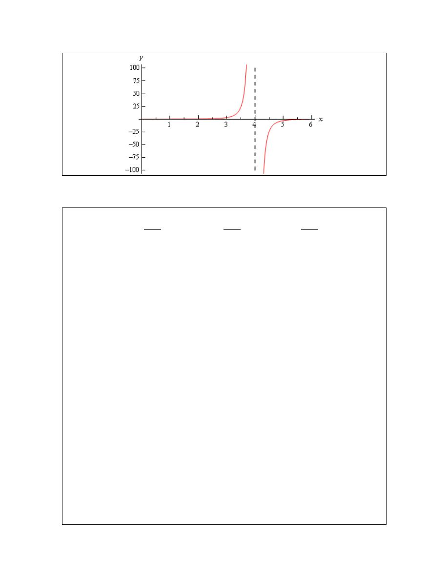
Calculus I
© 2007 Paul Dawkins
49
http://tutorial.math.lamar.edu/terms.aspx
All the examples to this point have had a constant in the numerator and we should probably take a
quick look at an example that doesn’t have a constant in the numerator.
Example 5
Evaluate each of the following limits.
3
3
3
2
2
2
lim
lim
lim
3
3
3
x
x
x
x
x
x
x
x
x
+
−
→
→
→
−
−
−
Solution
Let’s take a look at the right-handed limit first. For this limit we’ll have,
3
3
0
x
x
>
⇒
− >
The main difference here with this example is the behavior of the numerator as we let x get closer
and closer to 3. In this case we have the following behavior for both the numerator and
denominator.
3
0 and 2
6 as
3
x
x
x
− →
→
→
So, as we let x get closer and closer to 3 (always staying on the right of course) the numerator,
while not a constant, is getting closer and closer to a positive constant while the denominator is
getting closer and closer to zero, and will be positive since we are on the right side.
This means that we’ll have a numerator that is getting closer and closer to a non-zero and positive
constant divided by an increasingly smaller positive number and so the result should be an
increasingly larger positive number. The right-hand limit should then be positive infinity.
For the left-hand limit we’ll have,
3
3
0
x
x
<
⇒
− <
As with the right-hand limit we’ll have the following behaviors for the numerator and the
denominator,
3
0 and 2
6 as
3
x
x
x
− →
→
→
The main difference in this case is that the denominator will now be negative. So, we’ll have a
numerator that is approaching a positive, non-zero constant divided by an increasingly small
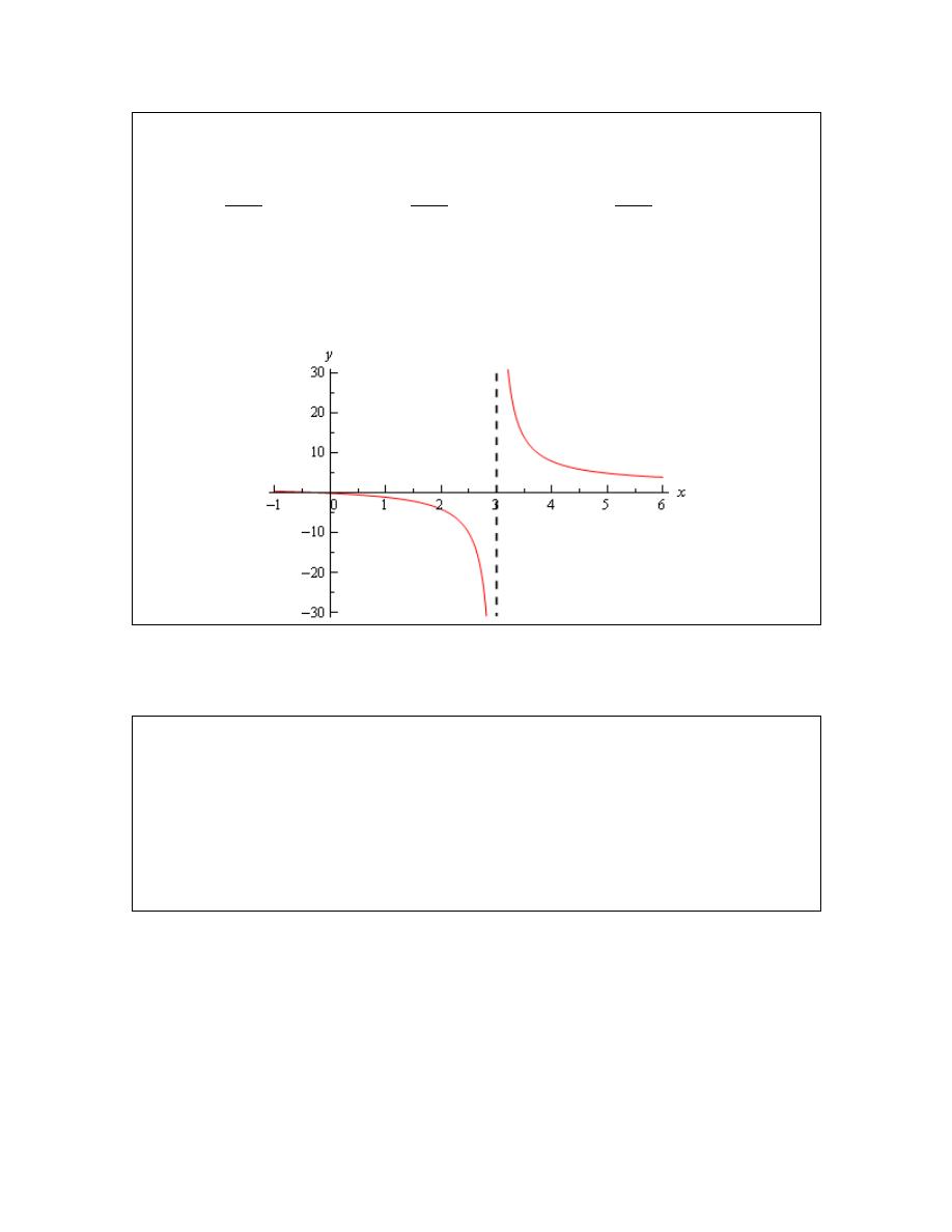
Calculus I
© 2007 Paul Dawkins
50
http://tutorial.math.lamar.edu/terms.aspx
negative number. The result will be an increasingly large and negative number.
The formal answers for this example are then,
3
3
3
2
2
2
lim
lim
lim
doesn't exist
3
3
3
x
x
x
x
x
x
x
x
x
+
−
→
→
→
= ∞
= −∞
−
−
−
As with most of the examples in this section the normal limit does not exist since the two one-
sided limits are not the same.
Here’s a quick graph to verify our limits.
So far all we’ve done is look at limits of rational expressions, let’s do a couple of quick examples
with some different functions.
Example 6
Evaluate
( )
0
lim ln
x
x
+
→
Solution
First, notice that we can only evaluate the right-handed limit here. We know that the domain of
any logarithm is only the positive numbers and so we can’t even talk about the left-handed limit
because that would necessitate the use of negative numbers. Likewise, since we can’t deal with
the left-handed limit then we can’t talk about the normal limit.
This limit is pretty simple to get from a quick sketch of the graph.
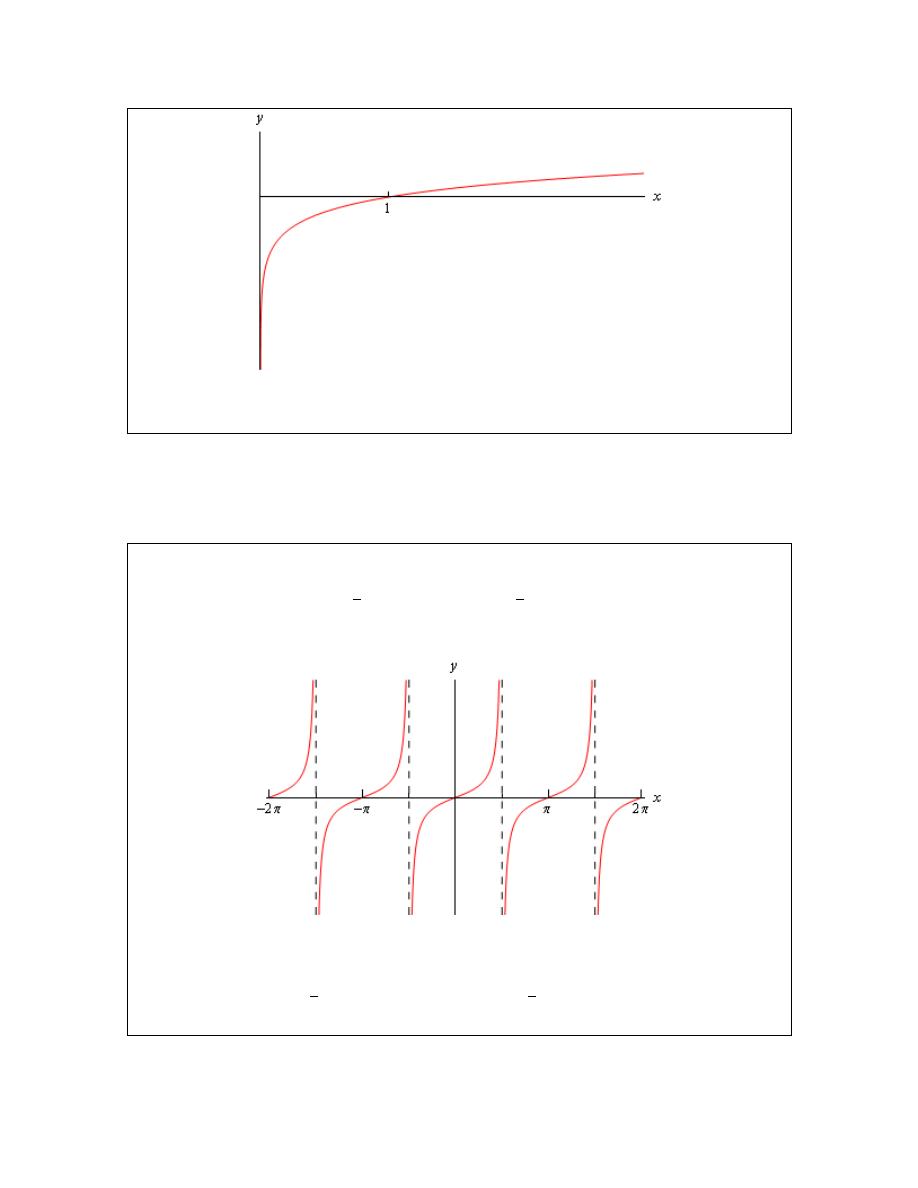
Calculus I
© 2007 Paul Dawkins
51
http://tutorial.math.lamar.edu/terms.aspx
From this we can see that,
( )
0
lim ln
x
x
+
→
= −∞
Example 7
Evaluate both of the following limits.
( )
( )
2
2
lim tan
lim tan
x
x
x
x
π
π
+
−
→
→
Solution
Here’s a quick sketch of the graph of the tangent function.
From this it’s easy to see that we have the following values for each of these limits,
( )
( )
2
2
lim tan
lim tan
x
x
x
x
π
π
+
−
→
→
= −∞
= ∞
Note that the normal limit will not exist because the two one-sided limits are not the same.
We’ll leave this section with a few facts about infinite limits.

Calculus I
© 2007 Paul Dawkins
52
http://tutorial.math.lamar.edu/terms.aspx
Facts
Given the functions
( )
f x and
( )
g x suppose we have,
( )
( )
lim
lim
x
c
x
c
f x
g x
L
→
→
= ∞
=
for some real numbers c and L. Then,
1.
( )
( )
lim
x
c
f x
g x
→
±
= ∞
2. If
0
L
>
then
( ) ( )
lim
x
c
f x g x
→
= ∞
3. If
0
L
<
then
( ) ( )
lim
x
c
f x g x
→
= −∞
4.
( )
( )
lim
0
x
c
g x
f x
→
=
To see the proof of this set of facts see the
Proof of Various Limit Properties
section in the Extras
chapter.
Note as well that the above set of facts also holds for one-sided limits. They will also hold if
( )
lim
x
c
f x
→
= −∞
, with a change of sign on the infinities in the first three parts. The proofs of
these changes to the facts are nearly identical to the proof of the original facts and so are left to
the reader.
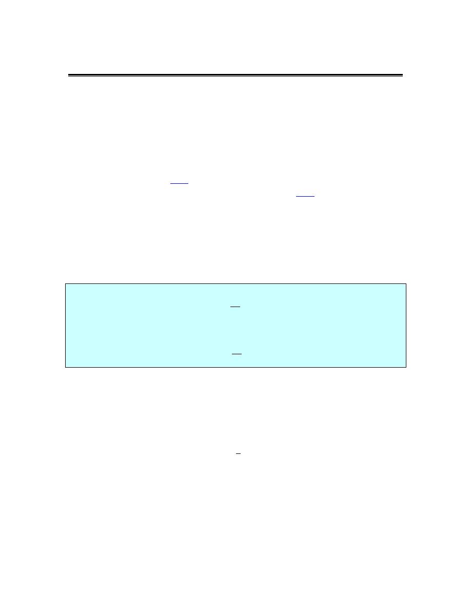
Calculus I
© 2007 Paul Dawkins
53
http://tutorial.math.lamar.edu/terms.aspx
Limits At Infinity, Part I
In the previous section we saw limits that were infinity and it’s now time to take a look at limits
at infinity. By limits at infinity we mean one of the following two limits.
( )
( )
lim
lim
x
x
f x
f x
→∞
→−∞
In other words, we are going to be looking at what happens to a function if we let x get very large
in either the positive or negative sense. Also, as we’ll soon see, these limits may also have
infinity as a value.
First, let’s note that the set of
Facts
from the Infinite Limit section also hold if the replace the
lim
x
c
→
with
lim
x
→∞
or
lim
x
→−∞
. The proof of this is nearly identical to the
proof
of the original set of
facts with only minor modifications to handle the change in the limit and so is left to the reader.
We won’t need these facts much over the next couple of sections but they will be required on
occasion.
In fact, many of the limits that we’re going to be looking at we will need the following two facts.
Fact 1
1. If r is a positive rational number and c is any real number then,
lim
0
r
x
c
x
→∞
=
2. If r is a positive rational number, c is any real number and x
r
is defined for
0
x
<
then,
lim
0
r
x
c
x
→−∞
=
The first part of this fact should make sense if you think about it. Because we are requiring
0
r
>
we know that x
r
will stay in the denominator. Next as we increase x then x
r
will also
increase. So, we have a constant divided by an increasingly large number and so the result will
be increasingly small. Or, in the limit we will get zero.
The second part is nearly identical except we need to worry about x
r
being defined for negative x.
This condition is here to avoid cases such as
1
2
r
=
. If this r were allowed then we’d be taking
the square root of negative numbers which would be complex and we want to avoid that at this
level.
Note as well that the sign of c will not affect the answer. Regardless of the sign of c we’ll still
have a constant divided by a very large number which will result in a very small number and the
larger x get the smaller the fraction gets. The sign of c will affect which direction the fraction
approaches zero (i.e. from the positive or negative side) but it still approaches zero.

Calculus I
© 2007 Paul Dawkins
54
http://tutorial.math.lamar.edu/terms.aspx
If you think about it this is really a special case of the last Fact from the
Facts
in the previous
section. However, to see a direct proof of this fact see the
Proof of Various Limit Properties
section in the Extras chapter.
Let’s start off the examples with one that will lead us to a nice idea that we’ll use on a regular
basis about limits at infinity for polynomials.
Example 1
Evaluate each of the following limits.
(a)
(
)
4
2
lim 2
8
x
x
x
x
→∞
−
−
[
Solution
]
(b)
(
)
5
3
2
1
3
lim
2
8
t
t
t
t
→−∞
+
− +
[
Solution
]
Solution
(a)
(
)
4
2
lim 2
8
x
x
x
x
→∞
−
−
Our first thought here is probably to just “plug” infinity into the polynomial and “evaluate” each
term to determine the value of the limit. It is pretty simple to see what each term will do in the
limit and so this seems like an obvious step, especially since we’ve been doing that for other
limits in previous sections.
So, let’s see what we get if we do that. As x approaches infinity, then x to a power can only get
larger and the coefficient on each term (the first and third) will only make the term even larger.
So, if we look at what each term is doing in the limit we get the following,
(
)
4
2
lim 2
8
x
x
x
x
→∞
−
−
= ∞ − ∞ − ∞
Now, we’ve got a small, but easily fixed, problem to deal with. We are probably tempted to say
that the answer is zero (because we have an infinity minus an infinity) or maybe
−∞
(because
we’re subtracting two infinities off of one infinity). However, in both cases we’d be wrong. This
is one of those indeterminate forms that we first started seeing in a previous
section
.
Infinities just don’t always behave as real numbers do when it comes to arithmetic. Without more
work there is simply no way to know what
∞ − ∞
will be and so we really need to be careful
with this kind of problem. To read a little more about this see the
Types of Infinity
section in the
Extras chapter.
So, we need a way to get around this problem. What we’ll do here is factor the largest power of x
out of the whole polynomial as follows,
(
)
4
2
4
2
3
1
8
lim 2
8
lim
2
x
x
x
x
x
x
x
x
→∞
→∞
−
−
=
−
−
If you’re not sure you agree with the factoring above (there’s a chance you haven’t really been
asked to do this kind of factoring prior to this) then recall that to check all you need to do is

Calculus I
© 2007 Paul Dawkins
55
http://tutorial.math.lamar.edu/terms.aspx
multiply the
4
x
back through the parenthesis to verify it was done correctly. Also, an easy way
to remember how to do this kind of factoring is to note that the second term is just the original
polynomial divided by
4
x
. This will always work when factoring a power of x out of a
polynomial.
Now for each of the terms we have,
4
2
3
1
8
lim
lim 2
2
x
x
x
x
x
→∞
→∞
= ∞
−
−
=
The first limit is clearly infinity and for the second limit we’ll use the fact above on the last two
terms. Therefore using
Fact 2
from the previous section we see value of the limit will be,
(
)
4
2
lim 2
8
x
x
x
x
→∞
−
−
= ∞
[
Return to Problems
]
(b)
(
)
5
3
2
1
3
lim
2
8
t
t
t
t
→−∞
+
− +
We’ll work this part much quicker than the previous part. All we need to do is factor out the
largest power of t to get the following,
(
)
5
3
2
5
1
3
2
3
5
1
2
1
8
lim
2
8
lim
3
t
t
t
t
t
t
t
t
t
→−∞
→−∞
+
− + =
+
− +
Remember that all you need to do to get the factoring correct is divide the original polynomial by
the power of t we’re factoring out,
5
t
in this case.
Now all we need to do is take the limit of the two terms. In the first don’t forget that since we’re
going out towards
−∞
and we’re raising t to the 5
th
power that the limit will be negative
(negative number raised to an odd power is still negative). In the second term we’ll again make
heavy use of the fact above to see that is a finite number.
Therefore, using the a modification of the
Facts
from the previous section the value of the limit is,
(
)
5
3
2
1
3
lim
2
8
t
t
t
t
→−∞
+
− + = −∞
[
Return to Problems
]
Okay, now that we’ve seen how a couple of polynomials work we can give a simple fact about
polynomials in general.
Fact 2
If
( )
1
1
1
0
n
n
n
n
p x
a x
a
x
a x
a
−
−
=
+
+ +
+
is a polynomial of degree n (i.e.
0
n
a
≠
) then,

Calculus I
© 2007 Paul Dawkins
56
http://tutorial.math.lamar.edu/terms.aspx
( )
( )
lim
lim
lim
lim
n
n
n
n
x
x
x
x
p x
a x
p x
a x
→∞
→∞
→−∞
→−∞
=
=
What this fact is really saying is that when we go to take a limit at infinity for a polynomial then
all we need to really do is look at the term with the largest power and ask what that term is doing
in the limit since the polynomial will have the same behavior.
You can see the proof in the
Proof of Various Limit Properties
section in the Extras chapter.
Let’s now move into some more complicated limits.
Example 2
Evaluate both of the following limits.
4
2
4
2
4
4
2
8
2
8
lim
lim
5
7
5
7
x
x
x
x
x
x
x
x
x
x
→∞
→−∞
−
+
−
+
−
+
−
+
Solution
First, the only difference between these two is that one is going to positive infinity and the other
is going to negative infinity. Sometimes this small difference will affect then value of the limit
and at other times it won’t.
Let’s start with the first limit and as with our first set of examples it might be tempting to just
“plug” in the infinity. Since both the numerator and denominator are polynomials we can use the
above fact to determine the behavior of each. Doing this gives,
4
2
4
2
8
lim
5
7
x
x
x
x
x
→∞
−
+
∞
=
−
+
−∞
This is yet another indeterminate form. In this case we might be tempted to say that the limit is
infinity (because of the infinity in the numerator), zero (because of the infinity in the
denominator) or -1 (because something divided by itself is one). There are three separate
arithmetic “rules” at work here and without work there is no way to know which “rule” will be
correct and to make matters worse it’s possible that none of them may work and we might get a
completely different answer, say
2
5
−
to pick a number completely at random.
So, when we have a polynomial divided by a polynomial we’re going to proceed much as we did
with only polynomials. We first identify the largest power of x in the denominator (and yes, we
only look at the denominator for this) and we then factor this out of both the numerator and
denominator. Doing this for the first limit gives,
4
4
2
2
3
4
4
4
1
8
2
2
8
lim
lim
7
5
7
5
x
x
x
x
x
x
x
x
x
x
x
→∞
→∞
−
+
−
+
=
−
+
− +
Once we’ve done this we can cancel the
4
x
from both the numerator and the denominator and

Calculus I
© 2007 Paul Dawkins
57
http://tutorial.math.lamar.edu/terms.aspx
then use the Fact 1 above to take the limit of all the remaining terms. This gives,
4
2
2
3
4
4
1
8
2
2
8
lim
lim
7
5
7
5
2 0 0
5 0
2
5
x
x
x
x
x
x
x
x
x
→∞
→∞
−
+
−
+
=
−
+
− +
+ +
=
− +
= −
In this case the indeterminate form was neither of the “obvious” choices of infinity, zero, or -1 so
be careful with make these kinds of assumptions with this kind of indeterminate forms.
The second limit is done in a similar fashion. Notice however, that nowhere in the work for the
first limit did we actually use the fact that the limit was going to plus infinity. In this case it
doesn’t matter which infinity we are going towards we will get the same value for the limit.
4
2
4
2
8
2
lim
5
7
5
x
x
x
x
x
→−∞
−
+
= −
−
+
In the previous example the infinity that we were using in the limit didn’t change the answer.
This will not always be the case so don’t make the assumption that this will always be the case.
Let’s take a look at an example where we get different answers for each limit.
Example 3
Evaluate each of the following limits.
2
2
3
6
3
6
lim
lim
5 2
5 2
x
x
x
x
x
x
→∞
→−∞
+
+
−
−
Solution
The square root in this problem won’t change our work, but it will make the work a little messier.
Let’s start with the first limit. In this case the largest power of x in the denominator is just an x.
So we need to factor an x out of the numerator and the denominator. When we are done factoring
the x out we will need an x in both of the numerator and the denominator. To get this in the
numerator we will have to factor an x
2
out of the square root so that after we take the square root
we will get an x.
This is probably not something you’re used to doing, but just remember that when it comes out of
the square root it needs to be an x and the only way have an x come out of a square is to take the
square root of x
2
and so that is what we’ll need to factor out of the term under the radical. Here’s
the factoring work for this part,

Calculus I
© 2007 Paul Dawkins
58
http://tutorial.math.lamar.edu/terms.aspx
2
2
2
2
2
6
3
3
6
lim
lim
5
5 2
2
6
3
lim
5
2
x
x
x
x
x
x
x
x
x
x
x
x
x
→∞
→∞
→∞
+
+
=
−
−
+
=
−
This is where we need to be really careful with the square root in the problem. Don’t forget that
2
x
x
=
Square roots are ALWAYS positive and so we need the absolute value bars on the x to make sure
that it will give a positive answer. This is not something that most people ever remember seeing
in an Algebra class and in fact it’s not always given in an Algebra class. However, at this point it
becomes absolutely vital that we know and use this fact. Using this fact the limit becomes,
2
2
6
3
3
6
lim
lim
5
5 2
2
x
x
x
x
x
x
x
x
→∞
→∞
+
+
=
−
−
Now, we can’t just cancel the x’s. We first will need to get rid of the absolute value bars. To do
this let’s recall the definition of absolute value.
if 0
if 0
x
x
x
x
x
≥
=
−
<
In this case we are going out to plus infinity so we can safely assume that the x will be positive
and so we can just drop the absolute value bars. The limit is then,
2
2
2
6
3
3
6
lim
lim
5
5 2
2
6
3
3 0
3
lim
5
0 2
2
2
x
x
x
x
x
x
x
x
x
x
x
→∞
→∞
→∞
+
+
=
−
−
+
+
=
=
= −
−
−
Let’s now take a look at the second limit (the one with negative infinity). In this case we will
need to pay attention to the limit that we are using. The initial work will be the same up until we
reach the following step.
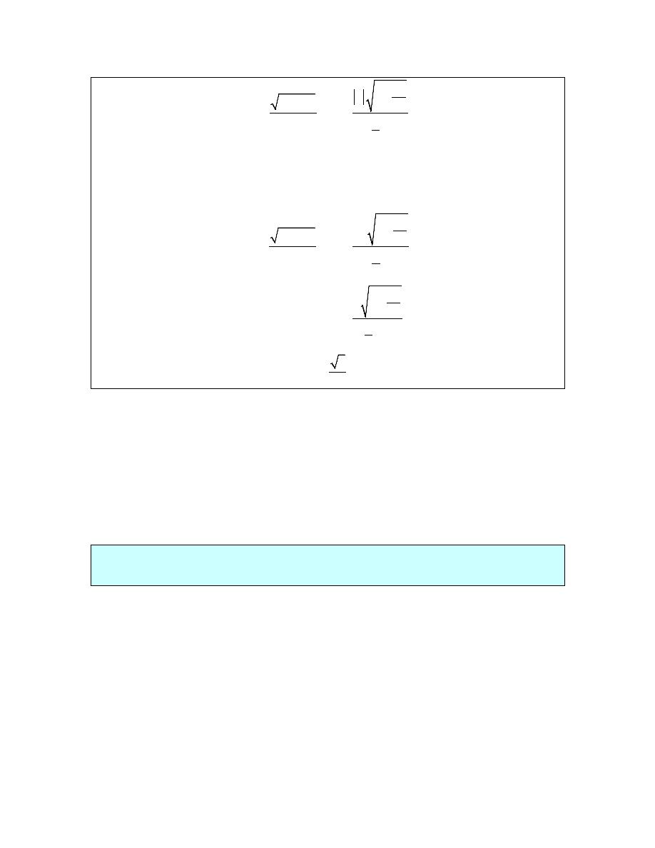
Calculus I
© 2007 Paul Dawkins
59
http://tutorial.math.lamar.edu/terms.aspx
2
2
6
3
3
6
lim
lim
5
5 2
2
x
x
x
x
x
x
x
x
→−∞
→−∞
+
+
=
−
−
In this limit we are going to minus infinity so in this case we can assume that x is negative. So, in
order to drop the absolute value bars in this case we will need to tack on a minus sign as well.
The limit is then,
2
2
2
6
3
3
6
lim
lim
5
5 2
2
6
3
lim
5
2
3
2
x
x
x
x
x
x
x
x
x
x
x
→−∞
→−∞
→−∞
−
+
+
=
−
−
−
+
=
−
=
So, as we saw in the last two examples sometimes the infinity in the limit will affect the answer
and other times it won’t. Note as well that it doesn’t always just change the sign of the number.
It can on occasion completely change the value. We’ll see an example of this later in this section.
Before moving on to a couple of more examples let’s revisit the idea of asymptotes that we first
saw in the previous section. Just as we can have vertical asymptotes defined in terms of limits we
can also have horizontal asymptotes defined in terms of limits.
Definition
The function f(x) will have a horizontal asymptote at y=L if either of the following are true.
( )
( )
lim
lim
x
x
f x
L
f x
L
→∞
→−∞
=
=
We’re not going to be doing much with asymptotes here, but it’s an easy fact to give and we can
use the previous example to illustrate all the asymptote ideas we’ve seen in the both this section
and the previous section. The function in the last example will have two horizontal asymptotes.
It will also have a vertical asymptote. Here is a graph of the function showing these.
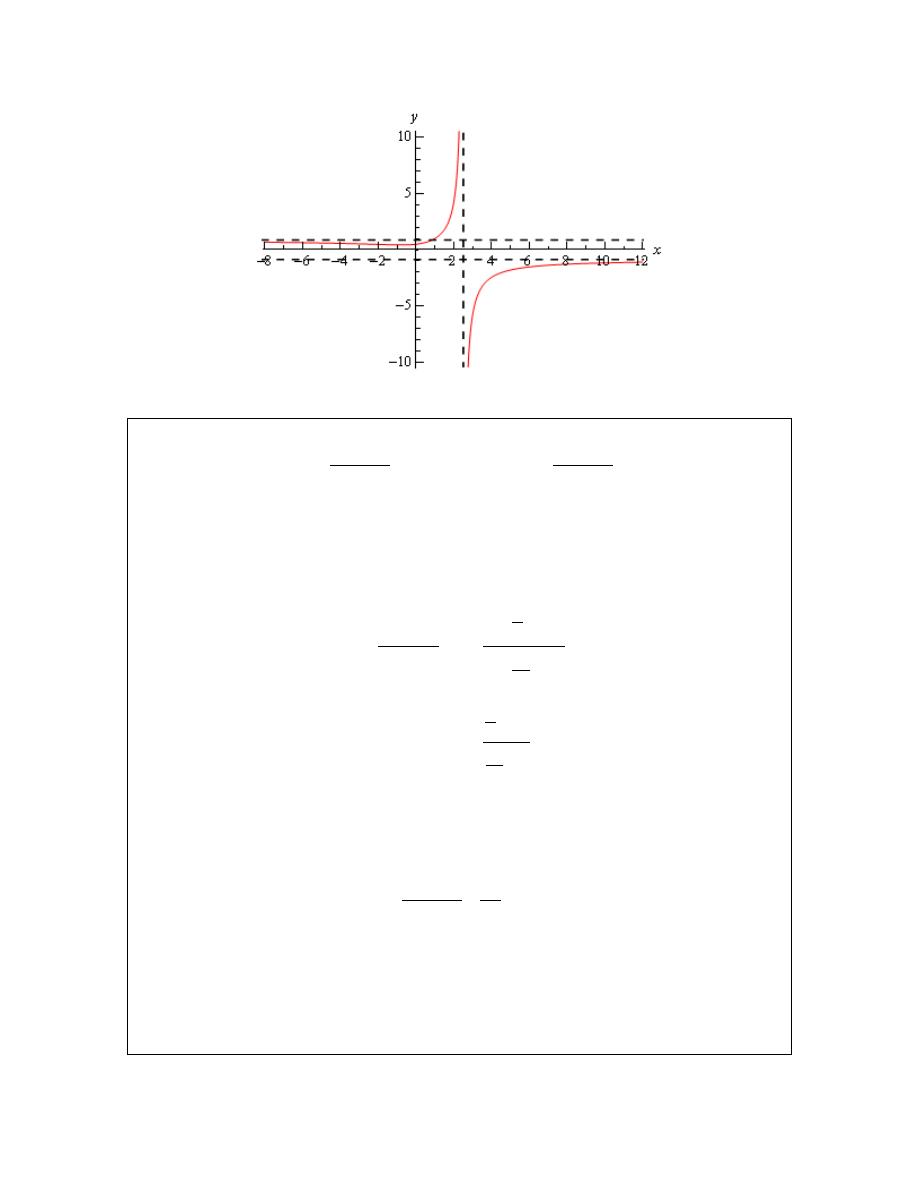
Calculus I
© 2007 Paul Dawkins
60
http://tutorial.math.lamar.edu/terms.aspx
Let’s work another couple of examples involving rational expressions.
Example 4
Evaluate each of the following limits.
2
6
2
6
3
3
4
4
lim
lim
1 5
1 5
z
z
z
z
z
z
z
z
→∞
→−∞
+
+
−
−
Solution
Let’s do the first limit and in this case it looks like we will factor a z
3
out of both the numerator
and denominator. Remember that we only look at the denominator when determining the largest
power of z here. There is a larger power of z in the numerator but we ignore it. We ONLY look
at the denominator when doing this! So doing the factoring gives,
3
3
2
6
3
3
3
3
3
4
4
lim
lim
1
1 5
5
4
lim
1
5
z
z
z
z
z
z
z
z
z
z
z
z
z
z
→∞
→∞
→∞
+
+
=
−
−
+
=
−
When we take the limit we’ll need to be a little careful. The first term in the numerator and
denominator will both be zero. However, the z
3
in the numerator will be going to plus infinity in
the limit and so the limit is,
2
6
3
4
lim
1 5
5
z
z
z
z
→∞
+
∞
=
= −∞
−
−
The final limit is negative because we have a quotient of positive quantity and a negative
quantity.
Now, let’s take a look at the second limit. Note that the only different in the work is at the final
“evaluation” step and so we’ll pick up the work there.

Calculus I
© 2007 Paul Dawkins
61
http://tutorial.math.lamar.edu/terms.aspx
3
2
6
3
3
4
4
lim
lim
1
1 5
5
5
z
z
z
z
z
z
z
z
→−∞
→−∞
+
+
−∞
=
=
= ∞
−
−
−
In this case the z
3
in the numerator gives negative infinity in the limit since we are going out to
minus infinity and the power is odd. The answer is positive since we have a quotient of two
negative numbers.
Example 5
Evaluate the following limit.
2
4
3
5
9
lim
2
3
t
t
t
t
t
→−∞
− −
+
Solution
In this case it looks like we will factor a
4
t
out of both the numerator and denominator. Doing
this gives,
4
2
2
3
4
4
3
4
2
3
4
1
5
9
5
9
lim
lim
3
2
3
2
1
5
9
lim
3
2
0
2
0
t
t
t
t
t
t
t
t
t
t
t
t
t
t
t
t
t
→−∞
→−∞
→−∞
− −
− −
=
+
+
− −
=
+
=
=
In this case using Fact 1 we can see that the numerator is zero and so since the denominator is
also not zero the fraction, and hence the limit, will be zero.
In this section we concentrated on limits at infinity with functions that only involved polynomials
and/or rational expression involving polynomials. There are many more types of functions that
we could use here. That is the subject of the next section.
To see a precise and mathematical definition of this kind of limit see the
The Definition of the
Limit
section at the end of this chapter.
Calculus I
© 2007 Paul Dawkins
62
http://tutorial.math.lamar.edu/terms.aspx
Limits At Infinity, Part II
In the previous section we looked at limits at infinity of polynomials and/or rational expression
involving polynomials. In this section we want to take a look at some other types of functions
that often show up in limits at infinity. The functions we’ll be looking at here are exponentials,
natural logarithms and inverse tangents.
Let’s start by taking a look at a some of very basic examples involving exponential functions.
Example 1
Evaluate each of the following limits.
lim
lim
lim
lim
x
x
x
x
x
x
x
x
−
−
→∞
→−∞
→∞
→−∞
e
e
e
e
Solution
There are really just restatements of facts given in the
basic exponential section
of the review so
we’ll leave it to you to go back and verify these.
lim
lim
0
lim
0
lim
x
x
x
x
x
x
x
x
−
−
→∞
→−∞
→∞
→−∞
= ∞
=
=
= ∞
e
e
e
e
The main point of this example was to point out that if the exponent of an exponential goes to
infinity in the limit then the exponential function will also go to infinity in the limit. Likewise, if
the exponent goes to minus infinity in the limit then the exponential will go to zero in the limit.
Here’s a quick set of examples to illustrate these ideas.
Example 2
Evaluate each of the following limits.
(a)
2
2 4
8
lim
x
x
x
−
→∞
−
e
[
Solution
]
(b)
4
2
5
1
lim
t
t
t
−
+
→−∞
e
[
Solution
]
(c)
1
0
lim
z
z
+
→
e
[
Solution
]
Solution
(a)
2
2 4
8
lim
x
x
x
−
→∞
−
e
In this part what we need to note (using Fact 2 above) is that in the limit the exponent of the
exponential does the following,
(
)
2
lim 2 4
8
x
x
x
→∞
−
−
= −∞
So, the exponent goes to minus infinity in the limit and so the exponential must go to zero in the
limit using the ideas from the previous set of examples. So, the answer here is,
2
2 4
8
lim
0
x
x
x
−
→∞
−
=
e
[
Return to Problems
]
Calculus I
© 2007 Paul Dawkins
63
http://tutorial.math.lamar.edu/terms.aspx
(b)
4
2
5
1
lim
t
t
t
−
+
→−∞
e
Here let’s first note that,
(
)
4
2
lim
5
1
t
t
t
→−∞
−
+ = ∞
The exponent goes to infinity in the limit and so the exponential will also need to go to infinity in
the limit. Or,
4
2
5
1
lim
t
t
t
−
+
→−∞
= ∞
e
[
Return to Problems
]
(c)
1
0
lim
z
z
+
→
e
On the surface this part doesn’t appear to belong in this section since it isn’t a limit at infinity.
However, it does fit into the ideas we’re examining in this set of examples.
So, let’s first note that using the idea from the previous section we have,
0
1
lim
z
z
+
→
= ∞
Remember that in order to do this limit here we do need to do a right hand limit.
So, the exponent goes to infinity in the limit and so the exponential must also go to infinity.
Here’s the answer to this part.
1
0
lim
z
z
+
→
= ∞
e
[
Return to Problems
]
Let’s work some more complicated examples involving exponentials. In the following set of
examples it won’t be that the exponents are more complicated, but instead that there will be more
than one exponential function to deal with.
Example 3
Evaluate each of the following limits.
(a)
(
)
10
6
2
15
lim
4
3
2
9
x
x
x
x
x
x
−
−
→∞
−
+
+
−
e
e
e
e
e
[
Solution
]
(b)
(
)
10
6
2
15
lim
4
3
2
9
x
x
x
x
x
x
−
−
→−∞
−
+
+
−
e
e
e
e
e
[
Solution
]
Solution
So, the only difference between these two limits is the fact that in the first we’re taking the limit
as we go to plus infinity and in the second we’re going to minus infinity. To this point we’ve
been able to “reuse” work from the first limit in the at least a portion of the second limit. With
exponentials that will often not be the case, we’re going to treat each of these as separate
problems.

Calculus I
© 2007 Paul Dawkins
64
http://tutorial.math.lamar.edu/terms.aspx
(a)
(
)
10
6
2
15
lim
4
3
2
9
x
x
x
x
x
x
−
−
→∞
−
+
+
−
e
e
e
e
e
Let’s start by just taking the limit of each of the pieces and see what we get.
(
)
10
6
2
15
lim
4
3
2
9
0 0
x
x
x
x
x
x
−
−
→∞
−
+
+
−
= ∞ − ∞ + ∞ + −
e
e
e
e
e
The last two terms aren’t any problem (they will be in the next part however, do you see that?).
The first three are a problem however as they present us with another indeterminate form.
When dealing with polynomials we factored out the term with the largest exponent in it. Let’s do
the same thing here. However, we now have to deal with both positive and negative exponents
and just what do we mean by the “largest” exponent. When dealing with these here we look at
the terms that are causing the problems and ask which is the largest exponent in those terms. So,
since only the first three terms are causing us problems (i.e. they all evaluate to an infinity in the
limit) we’ll look only at those.
So, since 10x is the largest of the three exponents there we’ll “factor” an
10
x
e
out of the whole
thing. Just as with polynomials we do the factoring by, in essence, dividing each term by
10
x
e
and remembering that to simply the division all we need to do is subtract the exponents. For
example, let’s just take a look at the last term,
15
15
10
25
10
9
9
9
x
x
x
x
x
−
−
−
−
−
= −
= −
e
e
e
e
Doing factoring on all terms then gives,
(
)
(
)
10
6
2
15
10
4
9
12
25
lim
4
3
2
9
lim
1 4
3
2
9
x
x
x
x
x
x
x
x
x
x
x
x
−
−
−
−
−
−
→∞
→∞
−
+
+
−
=
−
+
+
−
e
e
e
e
e
e
e
e
e
e
Notice that in doing this factoring all the remaining exponentials now have negative exponents
and we know that for this limit (i.e. going out to positive infinity) these will all be zero in the
limit and so will no longer cause problems.
We can now take the limit of the two factors. The first is clearly infinity and the second is clearly
a finite number (one in this case) and so the
Facts
from the Infinite Limits section gives us the
following limit,
(
)
10
6
2
15
lim
4
3
2
9
x
x
x
x
x
x
−
−
→∞
−
+
+
−
= ∞
e
e
e
e
e
To simplify the work here a little all we really needed to do was factor the
10
x
e
out of the
“problem” terms (the first three in this case) as follows,
(
)
(
)
( )( )
10
6
10
4
9
2
15
lim
4
3
lim
1 4
3
2
9
1
0 0
x
x
x
x
x
x
x
x
x
x
−
−
−
−
→∞
→∞
−
+
=
−
+
+
−
= ∞
+ −
= ∞
e
e
e
e
e
e
e
e

Calculus I
© 2007 Paul Dawkins
65
http://tutorial.math.lamar.edu/terms.aspx
We factored the
10
x
e
out of all terms for the practice of doing the factoring and to avoid any
issues with having the extra terms at the end. Note as well that while we wrote
( )( )
1
∞
for the
limit of the first term we are really using the
Facts
from the Infinite Limit section to do that limit.
[
Return to Problems
]
(b)
(
)
10
6
2
15
lim
4
3
2
9
x
x
x
x
x
x
−
−
→−∞
−
+
+
−
e
e
e
e
e
Let’s start this one off in the same manner as the first part. Let’s take the limit of each of the
pieces. This time note that because our limit is going to negative infinity the first three
exponentials will in fact go to zero (because their exponents go to minus infinity in the limit).
The final two exponentials will go to infinity in the limit (because their exponents go to plus
infinity in the limit).
Taking the limits gives,
(
)
10
6
2
15
lim
4
3
2
9
0 0 0
x
x
x
x
x
x
−
−
→−∞
−
+
+
−
= − + + ∞ − ∞
e
e
e
e
e
So, the last two terms are the problem here as they once again leave us with an indeterminate
form. As with the first example we’re going to factor out the “largest” exponent in the last two
terms. This time however, “largest” doesn’t refer to the bigger of the two numbers (-2 is bigger
than -15). Instead we’re going to use “largest” to refer to the exponent that is farther away from
zero. Using this definition of “largest” means that we’re going to factor an
15
x
−
e
out.
Again, remember that to factor this out all we really are doing is dividing each term by
15
x
−
e
and
then subtracting exponents. Here’s the work for the first term as an example,
(
)
10
10
15
25
15
x
x
x
x
x
− −
−
=
=
e
e
e
e
As with the first part we can either factor it out of only the “problem” terms (i.e. the last two
terms), or all the terms. For the practice we’ll factor it out of all the terms. Here is the factoring
work for this limit,
(
)
(
)
10
6
2
15
15
25
21
16
13
lim
4
3
2
9
lim
4
3
2
9
x
x
x
x
x
x
x
x
x
x
x
x
−
−
−
→−∞
→−∞
−
+
+
−
=
−
+
+
−
e
e
e
e
e
e
e
e
e
e
Finally, after taking the limit of the two terms (the first is infinity and the second is a negative,
finite number) and recalling the
Facts
from the Infinite Limit section we see that the limit is,
(
)
10
6
2
15
lim
4
3
2
9
x
x
x
x
x
x
−
−
→−∞
−
+
+
−
= −∞
e
e
e
e
e
[
Return to Problems
]
So, when dealing with sums and/or differences of exponential functions we look for the
exponential with the “largest” exponent and remember here that “largest” means the exponent
farthest from zero. Also remember that if we’re looking at a limit at plus infinity only the

Calculus I
© 2007 Paul Dawkins
66
http://tutorial.math.lamar.edu/terms.aspx
exponentials with positive exponents are going to cause problems so those are the only terms we
look at in determining the largest exponent. Likewise, if we are looking at a limit at minus
infinity then only exponentials with negative exponents are going to cause problems and so only
those are looked at in determining the largest exponent.
Finally, as you might have been able to guess from the previous example when dealing with a
sum and/or difference of exponentials all we need to do is look at the largest exponent to
determine the behavior of the whole expression. Again, remembering that if the limit is at plus
infinity we only look at exponentials with positive exponents and if we’re looking at a limit at
minus infinity we only look at exponentials with negative exponents.
Let’s next take a look at some rational functions involving exponentials.
Example 4
Evaluate each of the following limits.
(a)
4
2
4
2
6
lim
8
3
x
x
x
x
x
x
−
−
→∞
−
−
+
e
e
e
e
e
[
Solution
]
(b)
4
2
4
2
6
lim
8
3
x
x
x
x
x
x
−
−
→−∞
−
−
+
e
e
e
e
e
[
Solution
]
(c)
6
6
3
9
3
4
lim
2
5
t
t
t
t
t
t
−
−
−
→−∞
−
−
+
e
e
e
e
e
[
Solution
]
Solution
As with the previous example, the only difference between the first two parts is that one of the
limits is going to plus infinity and the other is going to minus infinity and just as with the
previous example each will need to be worked differently.
(a)
4
2
4
2
6
lim
8
3
x
x
x
x
x
x
−
−
→∞
−
−
+
e
e
e
e
e
The basic concept involved in working this problem is the same as with rational expressions in
the previous section. We look at the denominator and determine the exponential function with
the “largest” exponent which we will then factor out from both numerator and denominator. We
will use the same reasoning as we did with the previous example to determine the “largest”
exponent. In the case since we are looking at a limit at plus infinity we only look at exponentials
with positive exponents.
So, we’ll factor an
4
x
e
out of both then numerator and denominator. Once that is done we can
cancel the
4
x
e
and then take the limit of the remaining terms. Here is the work for this limit,

Calculus I
© 2007 Paul Dawkins
67
http://tutorial.math.lamar.edu/terms.aspx
(
)
(
)
4
6
4
2
4
2
4
2
5
6
2
5
6
6
lim
lim
8
3
8
3
6
lim
8
3
6 0
8 0 0
3
4
x
x
x
x
x
x
x
x
x
x
x
x
x
x
x
x
−
−
−
−
−
→∞
→∞
−
−
−
→∞
−
−
=
−
+
−
+
−
=
−
+
−
=
− +
=
e
e
e
e
e
e
e
e
e
e
e
e
e
[
Return to Problems
]
(b)
4
2
4
2
6
lim
8
3
x
x
x
x
x
x
−
−
→−∞
−
−
+
e
e
e
e
e
In this case we’re going to minus infinity in the limit and so we’ll look at exponentials in the
denominator with negative exponents in determining the “largest” exponent. There’s only one
however in this problem so that is what we’ll use.
Again, remember to only look at the denominator. Do NOT use the exponential from the
numerator, even though that one is “larger” than the exponential in the denominator. We always
look only at the denominator when determining what term to factor out regardless of what is
going on in the numerator.
Here is the work for this part.
(
)
(
)
4
2
4
2
5
5
3
5
5
3
6
6
lim
lim
8
3
8
3
6
lim
8
3
0
0 0 3
x
x
x
x
x
x
x
x
x
x
x
x
x
x
x
x
x
x
−
−
−
−
−
→−∞
→−∞
−
→−∞
−
−
=
−
+
−
+
−
=
−
+
− ∞
=
− +
= −∞
e
e
e
e
e
e
e
e
e
e
e
e
e
e
e
[
Return to Problems
]
(c)
6
6
3
9
3
4
lim
2
5
t
t
t
t
t
t
−
−
−
→−∞
−
−
+
e
e
e
e
e
We’ll do the work on this part with much less detail.

Calculus I
© 2007 Paul Dawkins
68
http://tutorial.math.lamar.edu/terms.aspx
(
)
(
)
9
15
3
6
6
3
9
3
9
12
6
15
3
12
6
4
4
lim
lim
2
5
2
5
4
lim
2
5
0 0
0 5 0
0
t
t
t
t
t
t
t
t
t
t
t
t
t
t
t
t
t
t
−
−
−
−
−
→−∞
→−∞
→−∞
−
−
=
−
+
− +
−
=
− +
−
=
− +
=
e
e
e
e
e
e
e
e
e
e
e
e
e
e
e
[
Return to Problems
]
Next, let’s take a quick look at some basic limits involving logarithms.
Example 5
Evaluate each of the following limits.
0
lim ln
lim ln
x
x
x
x
+
→∞
→
Solution
As with the last example I’ll leave it to you to verify these restatements from the
basic logarithm
section
.
0
lim ln
lim ln
x
x
x
x
+
→∞
→
= −∞
= ∞
Note that we had to do a right-handed limit for the first one since we can’t plug negative x’s into a
logarithm. This means that the normal limit won’t exist since we must look at x’s from both sides
of the point in question and x’s to the left of zero are negative.
From the previous example we can see that if the argument of a log (the stuff we’re taking the log
of) goes to zero from the right (i.e. always positive) then the log goes to negative infinity in the
limit while if the argument goes to infinity then the log also goes to infinity in the limit.
Note as well that we can’t look at a limit of a logarithm as x approaches minus infinity since we
can’t plug negative numbers into the logarithm.
Let’s take a quick look at some logarithm examples.
Example 6
Evaluate each of the following limits.
(a)
(
)
3
2
lim ln 7
1
x
x
x
→∞
−
+
[
Solution
]
(b)
2
1
lim ln
5
t
t
t
→−∞
−
[
Solution
]
Solution
(a)
(
)
3
2
lim ln 7
1
x
x
x
→∞
−
+
So, let’s first look to see what the argument of the log is doing,
Calculus I
© 2007 Paul Dawkins
69
http://tutorial.math.lamar.edu/terms.aspx
(
)
3
2
lim 7
1
x
x
x
→∞
−
+ = ∞
The argument of the log is going to infinity and so the log must also be going to infinity in the
limit. The answer to this part is then,
(
)
3
2
lim ln 7
1
x
x
x
→∞
−
+ = ∞
[
Return to Problems
]
(b)
2
1
lim ln
5
t
t
t
→−∞
−
First, note that the limit going to negative infinity here isn’t a violation (necessarily) of the fact
that we can’t plug negative numbers into the logarithm. The real issue is whether or not the
argument of the log will be negative or not.
Using the techniques from earlier in this section we can see that,
2
1
lim
0
5
t
t
t
→−∞
=
−
and let’s also note that for negative numbers (which we can assume we’ve got since we’re going
to minus infinity in the limit) the denominator will always be positive and so the quotient will
also always be positive. Therefore, not only does the argument go to zero, it goes to zero from
the right. This is exactly what we need to do this limit.
So, the answer here is,
2
1
lim ln
5
t
t
t
→−∞
= −∞
−
[
Return to Problems
]
As a final set of examples let’s take a look at some limits involving inverse tangents.
Example 7
Evaluate each of the following limits.
(a)
1
lim tan
x
x
−
→∞
[
Solution
]
(b)
1
lim tan
x
x
−
→−∞
[
Solution
]
(c)
(
)
1
3
lim tan
5
6
x
x
x
−
→∞
−
+
[
Solution
]
(d)
1
0
1
lim tan
x
x
−
−
→
[
Solution
]
Solution
The first two parts here are really just the basic limits involving inverse tangents and can easily be
found by examining the following sketch of inverse tangents. The remaining two parts are more
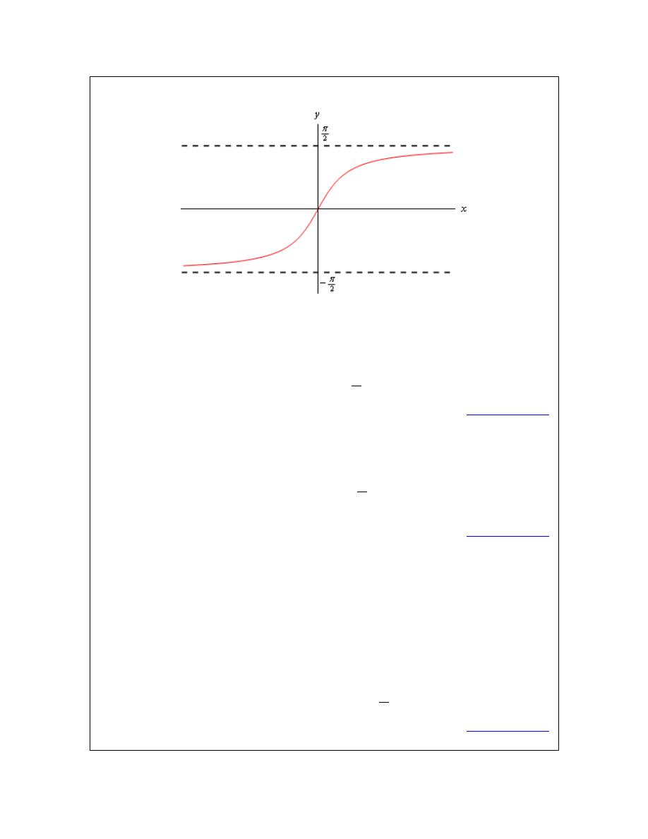
Calculus I
© 2007 Paul Dawkins
70
http://tutorial.math.lamar.edu/terms.aspx
involved but as with the exponential and logarithm limits really just refer back to the first two
parts as we’ll see.
(a)
1
lim tan
x
x
−
→∞
As noted above all we really need to do here is look at the graph of the inverse tangent. Doing
this shows us that we have the following value of the limit.
1
lim tan
2
x
x
π
−
→∞
=
[
Return to Problems
]
(b)
1
lim tan
x
x
−
→−∞
Again, not much to do here other than examine the graph of the inverse tangent.
1
lim tan
2
x
x
π
−
→−∞
= −
[
Return to Problems
]
(c)
(
)
1
3
lim tan
5
6
x
x
x
−
→∞
−
+
Okay, in part (a) above we saw that if the argument of the inverse tangent function (the stuff
inside the parenthesis) goes to plus infinity then we know the value of the limit. In this case
(using the techniques from the previous section) we have,
3
lim
5
6
x
x
x
→∞
−
+ = ∞
So, this limit is,
(
)
1
3
lim tan
5
6
2
x
x
x
π
−
→∞
−
+
=
[
Return to Problems
]

Calculus I
© 2007 Paul Dawkins
71
http://tutorial.math.lamar.edu/terms.aspx
(d)
1
0
1
lim tan
x
x
−
−
→
Even though this limit is not a limit at infinity we’re still looking at the same basic idea here.
We’ll use part (b) from above as a guide for this limit. We know from the
Infinite Limits
section
that we have the following limit for the argument of this inverse tangent,
0
1
lim
x
x
−
→
= −∞
So, since the argument goes to minus infinity in the limit we know that this limit must be,
1
0
1
lim tan
2
x
x
π
−
−
→
= −
[
Return to Problems
]
To see a precise and mathematical definition of this kind of limit see the
The Definition of the
Limit
section at the end of this chapter.

Calculus I
© 2007 Paul Dawkins
72
http://tutorial.math.lamar.edu/terms.aspx
Continuity
Over the last few sections we’ve been using the term “nice enough” to define those functions that
we could evaluate limits by just evaluating the function at the point in question. It’s now time to
formally define what we mean by “nice enough”.
Definition
A function
( )
f x
is said to be continuous at
x
a
=
if
( )
( )
lim
x
a
f x
f a
→
=
A function is said to be continuous on the interval [a, b] if it is continuous at each point in the
interval.
Note that this definition is also implicitly assuming that both
( )
f a
and
( )
lim
x
a
f x
→
exist. If
either of these do not exist then the function will not be continuous at
x
a
=
.
This definition can be turned around into the following fact.
Fact 1
If
( )
f x
is continuous at
x
a
=
then,
( )
( )
( )
( )
( )
( )
lim
lim
lim
x
a
x
a
x
a
f x
f a
f x
f a
f x
f a
−
+
→
→
→
=
=
=
This is exactly the same fact that we first put down
back
when we started looking at limits with
the exception that we have replaced the phrase “nice enough” with continuous.
It’s nice to finally know what we mean by “nice enough”, however, the definition doesn’t really
tell us just what it means for a function to be continuous. Let’s take a look at an example to help
us understand just what it means for a function to be continuous.
Example 1
Given the graph of f(x), shown below, determine if f(x) is continuous at
2
x
= −
,
0
x
=
, and
3
x
=
.
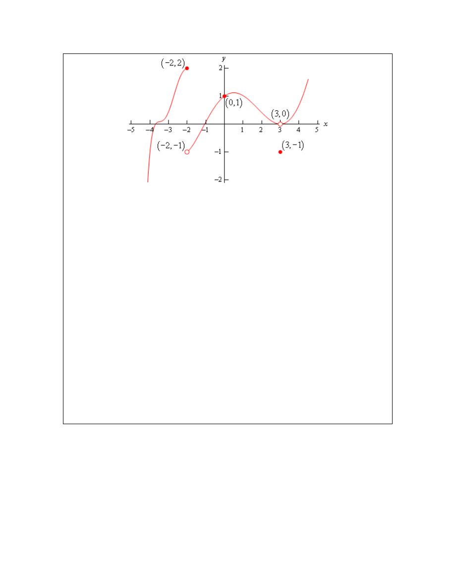
Calculus I
© 2007 Paul Dawkins
73
http://tutorial.math.lamar.edu/terms.aspx
Solution
To answer the question for each point we’ll need to get both the limit at that point and the
function value at that point. If they are equal the function is continuous at that point and if they
aren’t equal the function isn’t continuous at that point.
First
2
x
= −
.
( )
( )
2
2
2
lim
doesn't exist
x
f
f x
→−
− =
The function value and the limit aren’t the same and so the function is not continuous at this
point. This kind of discontinuity in a graph is called a jump discontinuity. Jump discontinuities
occur where the graph has a break in it as this graph does.
Now
0
x
=
.
( )
( )
0
0
1
lim
1
x
f
f x
→
=
=
The function is continuous at this point since the function and limit have the same value.
Finally
3
x
=
.
( )
( )
3
3
1
lim
0
x
f
f x
→
= −
=
The function is not continuous at this point. This kind of discontinuity is called a removable
discontinuity. Removable discontinuities are those where there is a hole in the graph as there is
in this case.
From this example we can get a quick “working” definition of continuity. A function is
continuous on an interval if we can draw the graph from start to finish without ever once picking
up our pencil. The graph in the last example has only two discontinuities since there are only two
places where we would have to pick up our pencil in sketching it.
In other words, a function is continuous if its graph has no holes or breaks in it.
For many functions it’s easy to determine where it won’t be continuous. Functions won’t be
continuous where we have things like division by zero or logarithms of zero. Let’s take a quick
look at an example of determining where a function is not continuous.

Calculus I
© 2007 Paul Dawkins
74
http://tutorial.math.lamar.edu/terms.aspx
Example 2
Determine where the function below is not continuous.
( )
2
4
10
2
15
t
h t
t
t
+
=
− −
Solution
Rational functions are continuous everywhere except where we have division by zero. So all that
we need to is determine where the denominator is zero. That’s easy enough to determine by
setting the denominator equal to zero and solving.
(
)(
)
2
2
15
5
3
0
t
t
t
t
− −
= −
+ =
So, the function will not be continuous at t=-3 and t=5.
A nice consequence of continuity is the following fact.
Fact 2
If
( )
f x
is continuous at
x
b
=
and
( )
lim
x
a
g x
b
→
=
then,
( )
(
)
( )
(
)
lim
lim
x
a
x
a
f g x
f
g x
→
→
=
To see a proof of this fact see the
Proof of Various Limit Properties
section in the Extras chapter.
With this fact we can now do limits like the following example.
Example 3
Evaluate the following limit.
0
sin
lim
x
x
→
e
Solution
Since we know that exponentials are continuous everywhere we can use the fact above.
0
0
0
lim sin
sin
lim
1
x
x
x
x
→
→
=
=
=
e
e
e
Another very nice consequence of continuity is the Intermediate Value Theorem.
Intermediate Value Theorem
Suppose that f(x) is continuous on [a, b] and let M be any number between f(a) and f(b). Then
there exists a number c such that,
1.
a
c
b
< <
2.
( )
f c
M
=
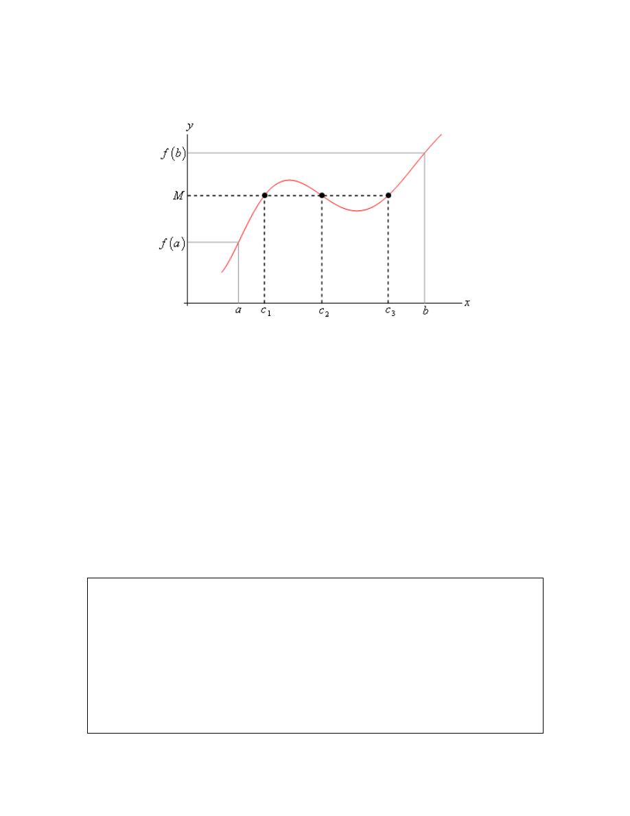
Calculus I
© 2007 Paul Dawkins
75
http://tutorial.math.lamar.edu/terms.aspx
All the Intermediate Value Theorem is really saying is that a continuous function will take on all
values between f(a) and f(b). Below is a graph of a continuous function that illustrates the
Intermediate Value Theorem.
As we can see from this image if we pick any value, M, that is between the value of f(a) and the
value of f(b) and draw a line straight out from this point the line will hit the graph in at least one
point. In other words somewhere between a and b the function will take on the value of M. Also,
as the figure shows the function may take on the value at more than one place.
It’s also important to note that the Intermediate Value Theorem only says that the function will
take on the value of M somewhere between a and b. It doesn’t say just what that value will be. It
only says that it exists.
So, the Intermediate Value Theorem tells us that a function will take the value of M somewhere
between a and b but it doesn’t tell us where it will take the value nor does it tell us how many
times it will take the value. There are important idea to remember about the Intermediate Value
Theorem.
A nice use of the Intermediate Value Theorem is to prove the existence of roots of equations as
the following example shows.
Example 4
Show that
( )
3
2
2
5
10
5
p x
x
x
x
=
−
−
+
has a root somewhere in the interval
[-1,2].
Solution
What we’re really asking here is whether or not the function will take on the value
( )
0
p x
=
somewhere between -1 and 2. In other words, we want to show that there is a number c such that
1
2
c
− < <
and
( )
0
p c
=
. However if we define
0
M
=
and acknowledge that
1
a
= −
and
2
b
=
we can see that these two condition on c are exactly the conclusions of the Intermediate
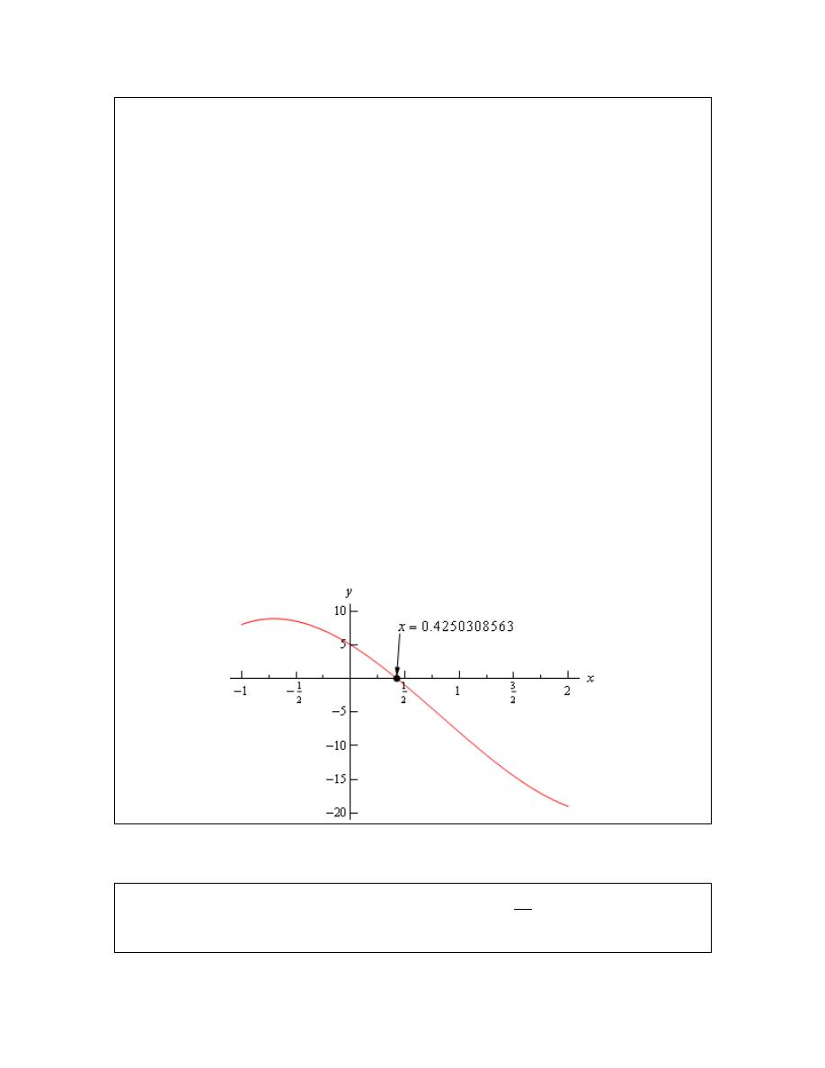
Calculus I
© 2007 Paul Dawkins
76
http://tutorial.math.lamar.edu/terms.aspx
Value Theorem.
So, this problem is set up to use the Intermediate Value Theorem and in fact, all we need to do is
to show that the function is continuous and that
0
M
=
is between
( )
1
p
−
and
( )
2
p
(i.e.
( )
( )
1
0
2
p
p
− < <
or
( )
( )
2
0
1
p
p
< <
−
and we’ll be done.
To do this all we need to do is compute,
( )
( )
1
8
2
19
p
p
− =
= −
So we have,
( )
( )
19
2
0
1
8
p
p
− =
< <
− =
Therefore
0
M
=
is between
( )
1
p
−
and
( )
2
p
and since
( )
p x
is a polynomial it’s continuous
everywhere and so in particular it’s continuous on the interval [-1,2]. So by the Intermediate
Value Theorem there must be a number
1
2
c
− < <
so that,
( )
0
p c
=
Therefore the polynomial does have a root between -1 and 2.
For the sake of completeness here is a graph showing the root that we just proved existed. Note
that we used a computer program to actually find the root and that the Intermediate Value
Theorem did not tell us what this value was.
Let’s take a look at another example of the Intermediate Value Theorem.
Example 5
If possible, determine if
( )
(
)
2
20 sin
3 cos
2
x
f x
x
=
+
takes the following values
in the interval [0,5].

Calculus I
© 2007 Paul Dawkins
77
http://tutorial.math.lamar.edu/terms.aspx
(a) Does
( )
10
f x
=
?
[
Solution
]
(b) Does
( )
10
f x
= −
?
[
Solution
]
Solution
Okay, so much as the previous example we’re being asked to determine, if possible, if the
function takes on either of the two values above in the interval [0,5]. First, let’s notice that this is
a continuous function and so we know that we can use the Intermediate Value Theorem to do this
problem.
Now, for each part we will let M be the given value for that part and then we’ll need to show that
M lives between
( )
0
f
and
( )
5
f
. If it does then we can use the Intermediate Value Theorem to
prove that the function will take the given value.
So, since we’ll need the two function evaluations for each part let’s give them here,
( )
( )
0
2.8224
5
19.7436
f
f
=
=
Now, let’s take a look at each part.
(a) Okay, in this case we’ll define
10
M
=
and we can see that,
( )
( )
0
2.8224 10 19.7436
5
f
f
=
<
<
=
So, by the Intermediate Value Theorem there must be a number
0
5
c
≤ ≤
such that
( )
10
f c
=
[
Return to Problems
]
(b) In this part we’ll define
10
M
= −
. We now have a problem. In this part M does not live
between
( )
0
f
and
( )
5
f
. So, what does this mean for us? Does this mean that
( )
10
f x
≠ −
in [0,5]?
Unfortunately for us, this doesn’t mean anything. It is possible that
( )
10
f x
≠ −
in [0,5], but is
it also possible that
( )
10
f x
= −
in [0,5]. The Intermediate Value Theorem will only tell us that
c’s will exist. The theorem will NOT tell us that c’s don’t exist.
In this case it is not possible to determine if
( )
10
f x
= −
in [0,5] using the Intermediate Value
Theorem.
[
Return to Problems
]
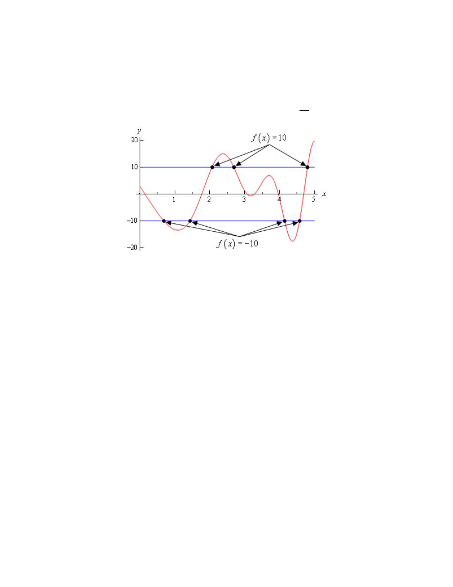
Calculus I
© 2007 Paul Dawkins
78
http://tutorial.math.lamar.edu/terms.aspx
Okay, as the previous example has shown, the Intermediate Value Theorem will not always be
able to tell us what we want to know. Sometimes we can use it to verify that a function will take
some value in a given interval and in other cases we won’t be able to use it.
For completeness sake here is the graph of
( )
(
)
2
20 sin
3 cos
2
x
f x
x
=
+
in the interval [0,5].
From this graph we can see that not only does
( )
10
f x
= −
in [0,5] it does so a total of 4 times!
Also note that as we verified in the first part of the previous example
( )
10
f x
=
in [0,5] and in
fact it does so a total of 3 times.
So, remember that the Intermediate Value Theorem will only verify that a function will take on a
given value. It will never exclude a value from being taken by the function. Also, if we can use
the Intermediate Value Theorem to verify that a function will take on a value it never tells us how
many times the function will take on the value, it only tells us that it does take the value.
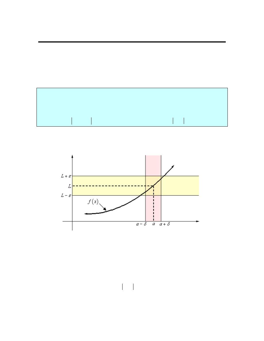
Calculus I
© 2007 Paul Dawkins
79
http://tutorial.math.lamar.edu/terms.aspx
The Definition of the Limit
In this section we’re going to be taking a look at the precise, mathematical definition of the three
kinds of limits we looked at in this chapter. We’ll be looking at the precise definition of limits at
finite points that have finite values, limits that are infinity and limits at infinity. We’ll also give
the precise, mathematical definition of continuity.
Let’s start this section out with the definition of a limit at a finite point that has a finite value.
Definition 1 Let f(x) be a function defined on an interval that contains
x
a
=
, except possibly at
x
a
=
. Then we say that,
( )
lim
x
a
f x
L
→
=
if for every number
0
ε
>
there is some number
0
δ
>
such that
( )
whenever
0
f x
L
x
a
ε
δ
− <
< − <
Wow. That’s a mouth full. Now that it’s written down, just what does this mean?
Let’s take a look at the following graph and let’s also assume that the limit does exist.
What the definition is telling us is that for any number
0
ε
>
that we pick we can go to our graph
and sketch two horizontal lines at
L
ε
+
and
L
ε
−
as shown on the graph above. Then
somewhere out there in the world is another number
0
δ
>
, which we will need to determine,
that will allow us to add in two vertical lines to our graph at
a
δ
+
and
a
δ
−
.
Now, if we take any x in the pink region, i.e. between
a
δ
+
and
a
δ
−
, then this x will be closer
to a than either of
a
δ
+
and
a
δ
−
. Or,
x a
δ
− <

Calculus I
© 2007 Paul Dawkins
80
http://tutorial.math.lamar.edu/terms.aspx
If we now identify the point on the graph that our choice of x gives then this point on the graph
will lie in the intersection of the pink and yellow region. This means that this function value f(x)
will be closer to L than either of
L
ε
+
and
L
ε
−
. Or,
( )
f x
L
ε
− <
So, if we take any value of x in the pink region then the graph for those values of x will lie in the
yellow region.
Notice that there are actually an infinite number of possible
δ
’s that we can choose. In fact, if we
go back and look at the graph above it looks like we could have taken a slightly larger
δ
and still
gotten the graph from that pink region to be completely contained in the yellow region.
Also, notice that as the definition points out we only need to make sure that the function is
defined in some interval around
x
a
=
but we don’t really care if it is defined at
x
a
=
.
Remember that limits do not care what is happening at the point, they only care what is
happening around the point in question.
Okay, now that we’ve gotten the definition out of the way and made an attempt to understand it
let’s see how it’s actually used in practice.
These are a little tricky sometimes and it can take a lot of practice to get good at these so don’t
feel too bad if you don’t pick up on this stuff right away. We’re going to be looking at a couple
of examples that work out fairly easily.
Example 1
Use the definition of the limit to prove the following limit.
2
0
lim
0
x
x
→
=
Solution
In this case both L and a are zero. So, let
0
ε
>
be any number. Don’t worry about what the
number is,
ε
is just some arbitrary number. Now according to the definition of the limit, if this
limit is to be true we will need to find some other number
0
δ
>
so that the following will be
true.
2
0
whenever
0
0
x
x
ε
δ
− <
< − <
Or upon simplifying things we need,
2
whenever
0
x
x
ε
δ
<
<
<
Often the way to go through these is to start with the left inequality and do a little simplification
and see if that suggests a choice for
δ
. We’ll start by bringing the exponent out of the absolute
value bars and then taking the square root of both sides.

Calculus I
© 2007 Paul Dawkins
81
http://tutorial.math.lamar.edu/terms.aspx
2
x
x
ε
ε
<
⇒
<
Now, the results of this simplification looks an awful lot like
0
x
δ
<
<
with the exception of
the “
0
<
” part. Missing that however isn’t a problem, it is just telling us that we can’t take
0
x
=
. So, it looks like if we choose
δ
ε
=
we should get what we want.
We’ll next need to verify that our choice of
δ
will give us what we want, i.e.,
2
whenever
0
x
x
ε
ε
<
<
<
Verification is in fact pretty much the same work that we did to get our guess. First, let’s again
let
0
ε
>
be any number and then choose
δ
ε
=
. Now, assume that
0
x
ε
<
<
. We need to
show that by choosing x to satisfy this we will get,
2
x
ε
<
To start the verification process we’ll start with
2
x
and then first strip out the exponent from the
absolute values. Once this is done we’ll use our assumption on x, namely that
x
ε
<
. Doing
all this gives,
( )
2
2
2
strip exponent out of absolute value bars
<
use the assumption that
simplify
x
x
x
ε
ε
ε
=
<
=
Or, upon taking the middle terms out, if we assume that
0
x
ε
<
<
then we will get,
2
x
ε
<
and this is exactly what we needed to show.
So, just what have we done? We’ve shown that if we choose
0
ε
>
then we can find a
0
δ
>
so
that we have,
2
0
whenever
0
0
x
x
ε
ε
− <
< − <
and according to our definition this means that,
2
0
lim
0
x
x
→
=
These can be a little tricky the first couple times through. Especially when it seems like we’ve
got to do the work twice. In the previous example we did some simplification on the left hand

Calculus I
© 2007 Paul Dawkins
82
http://tutorial.math.lamar.edu/terms.aspx
inequality to get our guess for
δ
and then seemingly went through exactly the same work to then
prove that our guess was correct. This is often how these work, although we will see an example
here in a bit where things don’t work out quite so nicely.
So, having said that let’s take a look at a slightly more complicated limit, although this one will
still be fairly similar to the first example.
Example 2
Use the definition of the limit to prove the following limit.
2
lim 5
4
6
x
x
→
− =
Solution
We’ll start this one out the same way that we did the first one. We won’t be putting in quite the
same amount of explanation however.
Let’s start off by letting
0
ε
>
be any number then we need to find a number
0
δ
>
so that the
following will be true.
(
)
5
4
6
whenever
0
2
x
x
ε
δ
− − <
< − <
We’ll start by simplifying the left inequality in an attempt to get a guess for
δ
. Doing this gives,
(
)
5
4
6
5
10
5
2
2
5
x
x
x
x
ε
ε
− − =
−
=
− <
⇒
− <
So, as with the first example it looks like if we do enough simplification on the left inequality we
get something that looks an awful lot like the right inequality and this leads us to choose
5
ε
δ
=
.
Let’s now verify this guess. So, again let
0
ε
>
be any number and then choose
5
ε
δ
=
. Next,
assume that
0
2
5
x
ε
δ
< − < =
and we get the following,
(
)
5
4
6
5
10
simplify things a little
5
2
more simplification....
5
use the assumption
5
5
and some more simplification
x
x
x
ε
ε
δ
ε
− − =
−
=
−
<
=
=
So, we’ve shown that
(
)
5
4
6
whenever
0
2
5
x
x
ε
ε
− − <
< − <
and so by our definition we have,
2
lim 5
4
6
x
x
→
− =

Calculus I
© 2007 Paul Dawkins
83
http://tutorial.math.lamar.edu/terms.aspx
Okay, so again the process seems to suggest that we have to essentially redo all our work twice,
once to make the guess for
δ
and then another time to prove our guess. Let’s do an example that
doesn’t work out quite so nicely.
Example 3
Use the definition of the limit to prove the following limit.
2
4
lim
11 9
x
x
x
→
+ − =
Solution
So, let’s get started. Let
0
ε
>
be any number then we need to find a number
0
δ
>
so that the
following will be true.
(
)
2
11
9
whenever
0
4
x
x
x
ε
δ
+ −
− <
< − <
We’ll start the guess process in the same manner as the previous two examples.
(
)
(
)(
)
2
2
11
9
20
5
4
5
4
x
x
x
x
x
x
x
x
ε
+ −
− =
+ −
=
+
−
= +
− <
Okay, we’ve managed to show that
(
)
2
11
9
x
x
ε
+ −
− <
is equivalent to
5
4
x
x
ε
+
− <
.
However, unlike the previous two examples, we’ve got an extra term in here that doesn’t show up
in the right inequality above. If we have any hope of proceeding here we’re going to need to find
some way to get rid of the
5
x
+
.
To do this let’s just note that if, by some chance, we can show that
5
x
K
+ <
for some number
K then, we’ll have the following,
5
4
4
x
x
K x
+
− <
−
If we now assume that what we really want to show is
4
K x
ε
− <
instead of
5
4
x
x
ε
+
− <
we get the following,
4
x
K
ε
− <
This is starting to seem familiar isn’t it?
All this work however, is based on the assumption that we can show that
5
x
K
+ <
for some K.
Without this assumption we can’t do anything so let’s see if we can do this.
Let’s first remember that we are working on a limit here and let’s also remember that limits are
only really concerned with what is happening around the point in question,
4
x
=
in this case.
So, it is safe to assume that whatever x is, it must be close to
4
x
=
. This means we can safely
assume that whatever x is, it is within a distance of, say one of
4
x
=
. Or in terms of an

Calculus I
© 2007 Paul Dawkins
84
http://tutorial.math.lamar.edu/terms.aspx
inequality, we can assume that,
4
1
x
− <
Why choose 1 here? There is no reason other than it’s a nice number to work with. We could
just have easily chosen 2, or 5, or
1
3
. The only difference our choice will make is on the actual
value of K that we end up with. You might want to go through this process with another choice
of K and see if you can do it.
So, let’s start with
4
1
x
− <
and get rid of the absolute value bars and this solve the resulting
inequality for x as follows,
1
4 1
3
5
x
x
− < − <
⇒
< <
If we now add 5 to all parts of this inequality we get,
8
5 10
x
< + <
Now, since
5
8
0
x
+ > >
(the positive part is important here) we can say that, provided
4
1
x
− <
we know that
5
5
x
x
+ = +
. Or, if take the double inequality above we have,
8
5
10
5
10
10
x
x
K
< + <
⇒
+ <
⇒
=
So, provided
4
1
x
− <
we can see that
5
10
x
+ <
which in turn gives us,
4
10
x
K
ε
ε
− <
=
So, to this point we make two assumptions about
4
x
−
We’ve assumed that,
4
AND
4
1
10
x
x
ε
− <
− <
It may not seem like it, but we’re now ready to chose a
δ
. In the previous examples we had only
a single assumption and we used that to give us
δ
. In this case we’ve got two and they BOTH
need to be true. So, we’ll let
δ
be the smaller of the two assumptions, 1 and
10
ε
.
Mathematically, this is written as,
min 1,
10
ε
δ
=
By doing this we can guarantee that,
AND
1
10
ε
δ
δ
≤
≤
Now that we’ve made our choice for
δ
we need to verify it. So,
0
ε
>
be any number and then

Calculus I
© 2007 Paul Dawkins
85
http://tutorial.math.lamar.edu/terms.aspx
choose
min 1,
10
ε
δ
=
. Assume that
0
4
min 1,
10
x
ε
δ
< − < =
. First, we get that,
0
4
4
10
10
x
x
ε
ε
δ
< − < ≤
⇒
− <
We also get,
0
4
1
4
1
5
10
x
x
x
δ
< − < ≤
⇒
− <
⇒
+ <
Finally, all we need to do is,
(
)
2
2
11
9
20
simplify things a little
5
4
factor
10
4
use the assumption that
5
10
10
use the assumption that
4
10
10
a little final simplification
x
x
x
x
x
x
x
x
x
ε
ε
ε
+ −
− =
+ −
= +
−
<
−
+ <
<
− <
<
We’ve now managed to show that,
(
)
2
11
9
whenever
0
4
min 1,
10
x
x
x
ε
ε
+ −
− <
< − <
and so by our definition we have,
2
4
lim
11 9
x
x
x
→
+ − =
Okay, that was a lot more work that the first two examples and unfortunately, it wasn’t all that
difficult of a problem. Well, maybe we should say that in comparison to some of the other limits
we could have tried to prove it wasn’t all that difficult. When first faced with these kinds of
proofs using the precise definition of a limit they can all seem pretty difficult.
Do not feel bad if you don’t get this stuff right away. It’s very common to not understand this
right away and to have to struggle a little to fully start to understand how these kinds of limit
definition proofs work.
Next, let’s give the precise definitions for the right- and left-handed limits.
Definition 2 For the right-hand limit we say that,
( )
lim
x
a
f x
L
+
→
=
if for every number
0
ε
>
there is some number
0
δ
>
such that
( )
(
)
whenever
0
or
f x
L
x a
a
x
a
ε
δ
δ
− <
< − <
< < +
Calculus I
© 2007 Paul Dawkins
86
http://tutorial.math.lamar.edu/terms.aspx
Definition 3 For the left-hand limit we say that,
( )
lim
x
a
f x
L
−
→
=
if for every number
0
ε
>
there is some number
0
δ
>
such that
( )
(
)
whenever
0
or
f x
L
x a
a
x
a
ε
δ
δ
− <
− < − <
− < <
Note that with both of these definitions there are two ways to deal with the restriction on x and
the one in parenthesis is probably the easier to use, although the main one given more closely
matches the definition of the normal limit above.
Let’s work a quick example of one of these, although as you’ll see they work in much the same
manner as the normal limit problems do.
Example 4
Use the definition of the limit to prove the following limit.
0
lim
0
x
x
+
→
=
Solution
Let
0
ε
>
be any number then we need to find a number
0
δ
>
so that the following will be true.
0
whenever
0
0
x
x
ε
δ
− <
< − <
Or upon a little simplification we need to show,
whenever
0
x
x
ε
δ
<
< <
As with the previous problems let’s start with the left hand inequality and see if we can’t use that
to get a guess for
δ
. The only simplification that we really need to do here is to square both
sides.
2
x
x
ε
ε
<
⇒
<
So, it looks like we can chose
2
δ ε
=
.
Let’s verify this. Let
0
ε
>
be any number and chose
2
δ ε
=
. Next assume that
2
0
x
ε
< <
.
This gives,
2
2
0
some quick simplification
use the assumption that
one final simplification
x
x
x
ε
ε
ε
− =
<
<
<
We now shown that,
2
0
whenever
0
0
x
x
ε
ε
− <
< − <
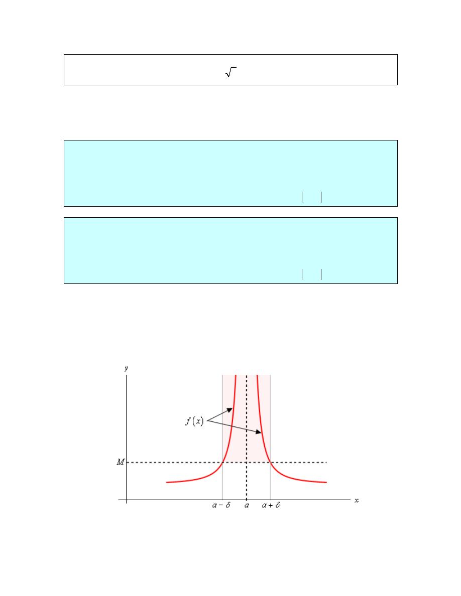
Calculus I
© 2007 Paul Dawkins
87
http://tutorial.math.lamar.edu/terms.aspx
and so by the definition of the right-hand limit we have,
0
lim
0
x
x
+
→
=
Let’s now move onto the definition of infinite limits. Here are the two definitions that we need to
cover both possibilities, limits that are positive infinity and limits that are negative infinity.
Definition 4 Let f(x) be a function defined on an interval that contains
x
a
=
, except possibly at
x
a
=
. Then we say that,
( )
lim
x
a
f x
→
= ∞
if for every number
0
M
>
there is some number
0
δ
>
such that
( )
whenever
0
f x
M
x a
δ
>
< − <
Definition 5 Let f(x) be a function defined on an interval that contains
x
a
=
, except possibly at
x
a
=
. Then we say that,
( )
lim
x
a
f x
→
= −∞
if for every number
0
N
<
there is some number
0
δ
>
such that
( )
whenever
0
f x
N
x a
δ
<
< − <
In these two definitions note that M must be a positive number and that N must be a negative
number. That’s an easy distinction to miss if you aren’t paying close attention.
Also note that we could also write down definitions for one-sided limits that are infinity if we
wanted to. We’ll leave that to you to do if you’d like to.
Here is a quick sketch illustrating Definition 4.
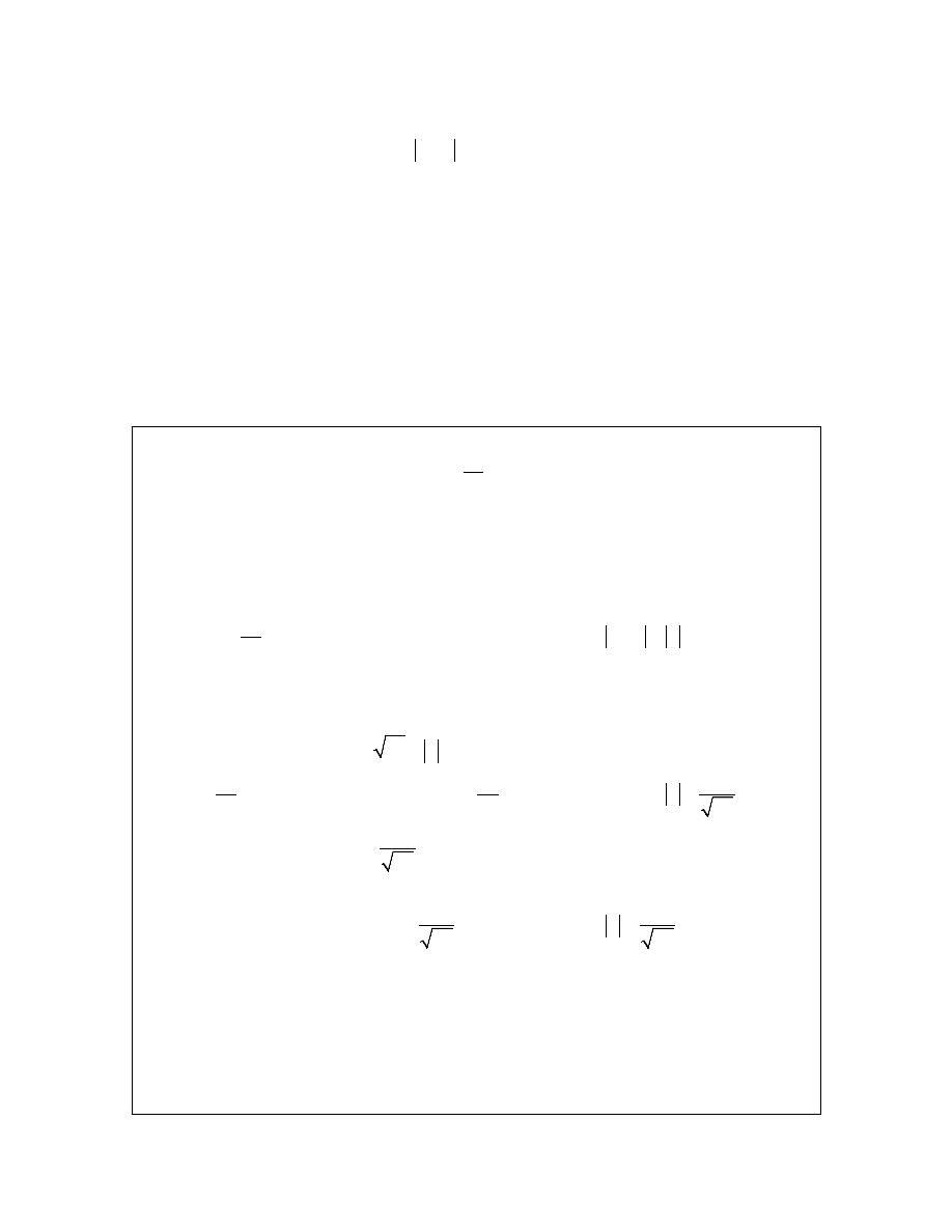
Calculus I
© 2007 Paul Dawkins
88
http://tutorial.math.lamar.edu/terms.aspx
What Definition 4 is telling us is that no matter how large we choose M to be we can always find
an interval around
x
a
=
, given by
0
x a
δ
< − <
for some number
δ
, so that as long as we
stay within that interval the graph of the function will be above the line
y
M
=
as shown in the
graph. Also note that we don’t need the function to actually exist at
x
a
=
in order for the
definition to hold. This is also illustrated in the sketch above.
Note as well that the larger M is the smaller we’re probably going to need to make
δ
.
To see an illustration of Definition 5 reflect the above graph about the x-axis and you’ll see a
sketch of Definition 5.
Let’s work a quick example of one of these to see how these differ from the previous examples.
Example 5
Use the definition of the limit to prove the following limit.
2
0
1
lim
x
x
→
= ∞
Solution
These work in pretty much the same manner as the previous set of examples do. The main
difference is that we’re working with an M now instead of an
ε
. So, let’s get going.
Let
0
M
>
be any number and we’ll need to choose a
0
δ
>
so that,
2
1
whenever
0
0
M
x
x
x
δ
>
< − =
<
As with the all the previous problems we’ll start with the left inequality and try to get something
in the end that looks like the right inequality. To do this we’ll basically solve the left inequality
for x and we’ll need to recall that
2
x
x
=
. So, here’s that work.
2
2
1
1
1
M
x
x
x
M
M
>
⇒
<
⇒
<
So, it looks like we can chose
1
M
δ =
. All we need to do now is verify this guess.
Let
0
M
>
be any number, choose
1
M
δ =
and assume that
1
0
x
M
<
<
.
In the previous examples we tried to show that our assumptions satisfied the left inequality by
working with it directly. However, in this, the function and our assumption on x that we’ve got
actually will make this easier to start with the assumption on x and show that we can get the left
inequality out of that. Note that this is being done this way mostly because of the function that
we’re working with and not because of the type of limit that we’ve got.
Calculus I
© 2007 Paul Dawkins
89
http://tutorial.math.lamar.edu/terms.aspx
Doing this work gives,
2
2
2
2
2
2
1
1
square both sides
1
acknowledge that
1
solve for
x
M
x
M
x
x
x
M
M
x
x
<
<
<
=
>
So, we’ve managed to show that,
2
1
1
whenever
0
0
M
x
x
M
>
< − <
and so by the definition of the limit we have,
2
0
1
lim
x
x
→
= ∞
For our next set of limit definitions let’s take a look at the two definitions for limits at infinity.
Again, we need one for a limit at plus infinity and another for negative infinity.
Definition 6 Let f(x) be a function defined on
x
K
>
for some K. Then we say that,
( )
lim
x
f x
L
→∞
=
if for every number
0
ε
>
there is some number
0
M
>
such that
( )
whenever
f x
L
x
M
ε
− <
>
Definition 7 Let f(x) be a function defined on
x
K
<
for some K. Then we say that,
( )
lim
x
f x
L
→−∞
=
if for every number
0
ε
>
there is some number
0
N
<
such that
( )
whenever
f x
L
x
N
ε
− <
<
To see what these definitions are telling us here is a quick sketch illustrating Definition 6.
Definition 6 tells us is that no matter how close to L we want to get, mathematically this is given
by
( )
f x
L
ε
− <
for any chosen
ε
, we can find another number M such that provided we take
any x bigger than M, then the graph of the function for that x will be closer to L than either
L
ε
−
and
L
ε
+
. Or, in other words, the graph will be in the shaded region as shown in the sketch
below.
Finally, note that the smaller we make
ε
the larger we’ll probably need to make M.
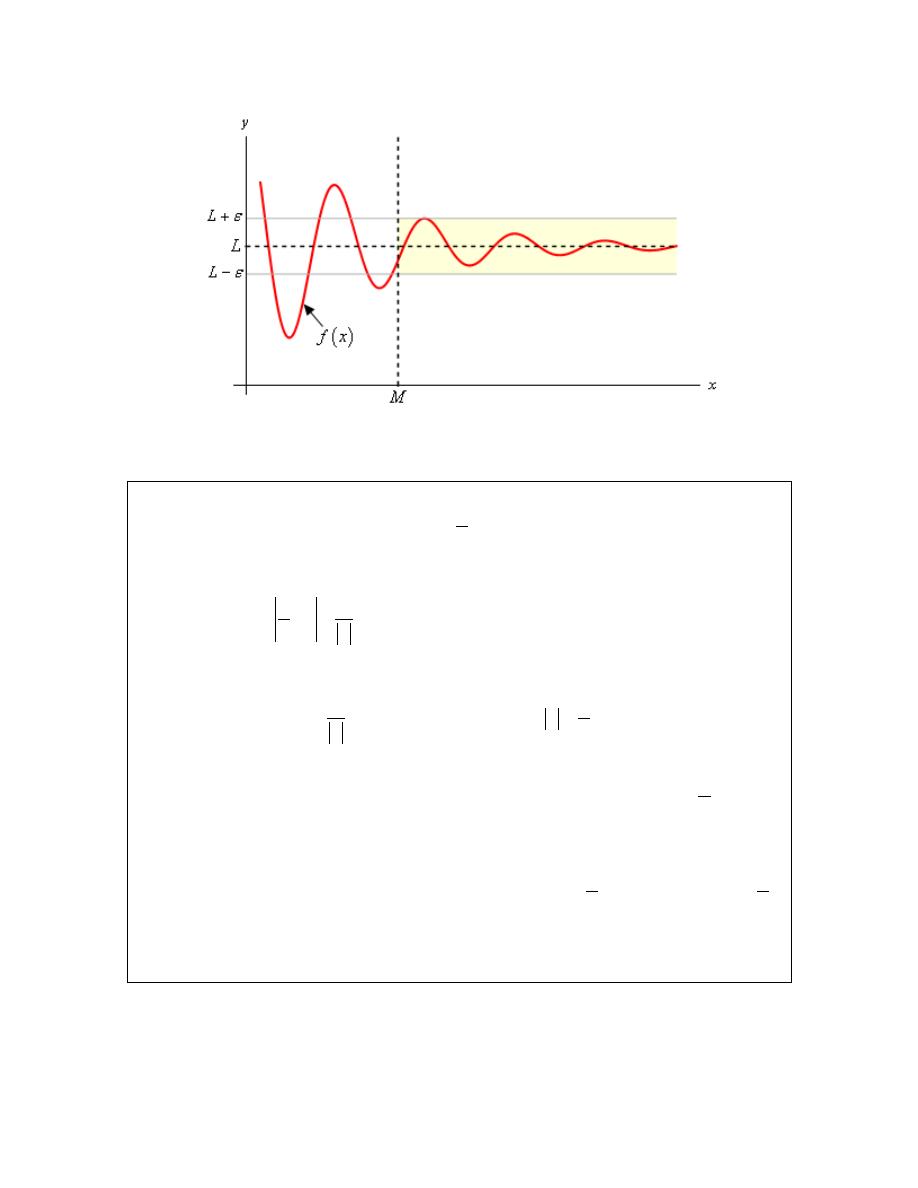
Calculus I
© 2007 Paul Dawkins
90
http://tutorial.math.lamar.edu/terms.aspx
Here’s a quick example of one of these limits.
Example 6
Use the definition of the limit to prove the following limit.
1
lim
0
x
x
→−∞
=
Solution
Let
0
ε
>
be any number and we’ll need to choose a
0
N
<
so that,
1
1
0
whenever
x
N
x
x
ε
− =
<
<
Getting our guess for N isn’t too bad here.
1
1
x
x
ε
ε
<
⇒
>
Since we’re heading out towards negative infinity it looks like we can choose
1
N
ε
= −
. Note
that we need the “-” to make sure that N is negative (recall that
0
ε
>
).
Let’s verify that our guess will work. Let
0
ε
>
and choose
1
N
ε
= −
and assume that
1
x
ε
< −
.
As with the previous example the function that we’re working with here suggests that it will be
easier to start with this assumption and show that we can get the left inequality out of that.
Calculus I
© 2007 Paul Dawkins
91
http://tutorial.math.lamar.edu/terms.aspx
1
1
take the absolute value
1
do a little simplification
1
solve for
1
0
rewrite things a little
x
x
x
x
x
x
ε
ε
ε
ε
ε
< −
> −
>
<
− <
Note that when we took the absolute value of both sides we changed both sides from negative
numbers to positive numbers and so also had to change the direction of the inequality.
So, we’ve shown that,
1
1
1
0
whenever
x
x
x
ε
ε
− =
<
< −
and so by the definition of the limit we have,
1
lim
0
x
x
→−∞
=
For our final limit definition let’s look at limits at infinity that are also infinite in value. There are
four possible limits to define here. We’ll do one of them and leave the other three to you to write
down if you’d like to.
Definition 8 Let f(x) be a function defined on
x
K
>
for some K. Then we say that,
( )
lim
x
f x
→∞
= ∞
if for every number
0
N
>
there is some number
0
M
>
such that
( )
whenever
f x
N
x
M
>
>
The other three definitions are almost identical. The only differences are the signs of M and/or N
and the corresponding inequality directions.
As a final definition in this section let’s recall that we previously said that a function was
continuous if,
( )
( )
lim
x
a
f x
f a
→
=
So, since continuity, as we previously defined it, is defined in terms of a limit we can also now
give a more precise definition of continuity. Here it is,

Calculus I
© 2007 Paul Dawkins
92
http://tutorial.math.lamar.edu/terms.aspx
Definition 9 Let f(x) be a function defined on an interval that contains
x
a
=
. Then we say that
f(x) is continuous at
x
a
=
if for every number
0
ε
>
there is some number
0
δ
>
such that
( )
( )
whenever
0
f x
f a
x
a
ε
δ
−
<
< − <
This definition is very similar to the first definition in this section and of course that should make
some sense since that is exactly the kind of limit that we’re doing to show that a function is
continuous. The only real difference is that here we need to make sure that the function is
actually defined at
x
a
=
, while we didn’t need to worry about that for the first definition since
limits don’t really care what is happening at the point.
We won’t do any examples of proving a function is continuous at a point here mostly because
we’ve already done some examples. Go back and look at the first three examples. In each of
these examples the value of the limit was the value of the function evaluated at
x
a
=
and so in
each of these examples not only did we prove the value of the limit we also managed to prove
that each of these functions are continuous at the point in question.

Calculus I
© 2007 Paul Dawkins
93
http://tutorial.math.lamar.edu/terms.aspx