Calculus I review pdf - عبدالرحمن سهيل

CALCULUS I

Review

Paul Dawkins

Calculus I

Table of Contents

Preface ............................................................................................................................................ ii

Review............................................................................................................................................. 1

Introduction ................................................................................................................................................ 1

Review : Functions ..................................................................................................................................... 3

Review : Inverse Functions .......................................................................................................................13

Review : Trig Functions ............................................................................................................................20

Review : Solving Trig Equations ..............................................................................................................27

Review : Solving Trig Equations with Calculators, Part I ........................................................................36

Review : Solving Trig Equations with Calculators, Part II .......................................................................47

Review : Exponential Functions ...............................................................................................................52

Review : Logarithm Functions ..................................................................................................................55

Review : Exponential and Logarithm Equations .......................................................................................61

Review : Common Graphs ........................................................................................................................67

http://tutorial.math.lamar.edu/terms.aspx

Calculus I

Preface

Here are my online notes for my Calculus I course that I teach here at Lamar University. Despite
the fact that these are my “class notes”, they should be accessible to anyone wanting to learn
Calculus I or needing a refresher in some of the early topics in calculus.

I’ve tried to make these notes as self contained as possible and so all the information needed to
read through them is either from an Algebra or Trig class or contained in other sections of the
notes.

Here are a couple of warnings to my students who may be here to get a copy of what happened on
a day that you missed.

1. Because I wanted to make this a fairly complete set of notes for anyone wanting to learn

calculus I have included some material that I do not usually have time to cover in class
and because this changes from semester to semester it is not noted here. You will need to
find one of your fellow class mates to see if there is something in these notes that wasn’t
covered in class.

2. Because I want these notes to provide some more examples for you to read through, I

don’t always work the same problems in class as those given in the notes. Likewise, even
if I do work some of the problems in here I may work fewer problems in class than are
presented here.

3. Sometimes questions in class will lead down paths that are not covered here. I try to

anticipate as many of the questions as possible when writing these up, but the reality is
that I can’t anticipate all the questions. Sometimes a very good question gets asked in
class that leads to insights that I’ve not included here. You should always talk to
someone who was in class on the day you missed and compare these notes to their notes
and see what the differences are.

4. This is somewhat related to the previous three items, but is important enough to merit its

own item. THESE NOTES ARE NOT A SUBSTITUTE FOR ATTENDING CLASS!!
Using these notes as a substitute for class is liable to get you in trouble. As already noted
not everything in these notes is covered in class and often material or insights not in these
notes is covered in class.

http://tutorial.math.lamar.edu/terms.aspx

Calculus I

Review

Introduction

Technically a student coming into a Calculus class is supposed to know both Algebra and
Trigonometry. The reality is often much different however. Most students enter a Calculus class
woefully unprepared for both the algebra and the trig that is in a Calculus class. This is very
unfortunate since good algebra skills are absolutely vital to successfully completing any Calculus
course and if your Calculus course includes trig (as this one does) good trig skills are also
important in many sections.

The intent of this chapter is to do a very cursory review of some algebra and trig skills that are
absolutely vital to a calculus course. This chapter is not inclusive in the algebra and trig skills
that are needed to be successful in a Calculus course. It only includes those topics that most
students are particularly deficient in. For instance factoring is also vital to completing a standard
calculus class but is not included here. For a more in depth review you should visit my
Algebra/Trig review or my full set of Algebra notes at

http://tutorial.math.lamar.edu

Note that even though these topics are very important to a Calculus class I rarely cover all of
these in the actual class itself. We simply don’t have the time to do that. I do cover certain
portions of this chapter in class, but for the most part I leave it to the students to read this chapter
on their own.

Here is a list of topics that are in this chapter. I’ve also denoted the sections that I typically cover
during the first couple of days of a Calculus class.

Review : Functions

– Here is a quick review of functions, function notation and a couple of

fairly important ideas about functions.

Review : Inverse Functions

– A quick review of inverse functions and the notation for inverse

functions.

Review : Trig Functions

– A review of trig functions, evaluation of trig functions and the unit

circle. This section usually gets a quick review in my class.

Review : Solving Trig Equations

– A reminder on how to solve trig equations. This section is

always covered in my class.

Review : Solving Trig Equations with Calculators, Part I

– The previous section worked

problem whose answers were always the “standard” angles. In this section we work some

http://tutorial.math.lamar.edu/terms.aspx

Calculus I

problems whose answers are not “standard” and so a calculator is needed. This section is always
covered in my class as most trig equations in the remainder will need a calculator.

Review : Solving Trig Equations with Calculators, Part II

– Even more trig equations

requiring a calculator to solve.

Review : Exponential Functions

– A review of exponential functions. This section usually gets

a quick review in my class.

Review : Logarithm Functions

– A review of logarithm functions and logarithm properties.

This section usually gets a quick review in my class.

Review : Exponential and Logarithm Equations

– How to solve exponential and logarithm

equations. This section is always covered in my class.

Review : Common Graphs

– This section isn’t much. It’s mostly a collection of graphs of many

of the common functions that are liable to be seen in a Calculus class.

http://tutorial.math.lamar.edu/terms.aspx

Calculus I

Review : Functions

In this section we’re going to make sure that you’re familiar with functions and function notation.
Both will appear in almost every section in a Calculus class and so you will need to be able to
deal with them.

First, what exactly is a function? An equation will be a function if for any x in the domain of the
equation (the domain is all the x’s that can be plugged into the equation) the equation will yield
exactly one value of y.

This is usually easier to understand with an example.

Example 1

Determine if each of the following are functions.

(a)

(b)

= +

Solution
(a) This first one is a function. Given an x, there is only one way to square it and then add 1 to
the result. So, no matter what value of x you put into the equation, there is only one possible
value of y.

(b)  The only difference between this equation and the first is that we moved the exponent off the
x and onto the y.  This small change is all that is required, in this case, to change the equation
from a function to something that isn’t a function.

To see that this isn’t a function is fairly simple. Choose a value of x, say x=3 and plug this into
the equation.

3 1

= + =

Now, there are two possible values of y that we could use here. We could use

= −

Since there are two possible values of y that we get from a single x this equation isn’t a function.

Note that this only needs to be the case for a single value of x to make an equation not be a
function. For instance we could have used x=-1 and in this case we would get a single y (y=0).
However, because of what happens at x=3 this equation will not be a function.

Next we need to take a quick look at function notation. Function notation is nothing more than a
fancy way of writing the y in a function that will allow us to simplify notation and some of our
work a little.

Let’s take a look at the following function.

−

Using function notation we can write this as any of the following.

http://tutorial.math.lamar.edu/terms.aspx

Calculus I

( )

f x

g x

h x

R x

w x

y x

−



Recall that this is NOT a letter times x, this is just a fancy way of writing y.

So, why is this useful? Well let’s take the function above and let’s get the value of the function at
x=-3. Using function notation we represent the value of the function at x=-3 as f(-3). Function
notation gives us a nice compact way of representing function values.

Now, how do we actually evaluate the function? That’s really simple. Everywhere we see an x
on the right side we will substitute whatever is in the parenthesis on the left side. For our
function this gives,

( ) ( )

( )

2 9

15 3

− =

−

− − +

+ +

Let’s take a look at some more function evaluation.

Example 2

Given

( )

f x

= − +

−

find each of the following.

(a)

( )

[

Solution

]

(b)

(

)

−

[

Solution

]

(c)

( )

f t

[

Solution

]

(d)

(

)

f t

−

[

Solution

]

(e)

(

)

f x

−

[

Solution

]

(f)

(

)

−

[

Solution

]

Solution

(a)

( )

6(2) 11

= −

− = −

[

Return to Problems

]

(b)

(

)

(

)

(

)

100 60 11

171

−

= − −

+ −

− = −

−

− = −

Be careful when squaring negative numbers!

[

Return to Problems

]

(c)

( )

f t

= − + −

Remember that we substitute for the x’s WHATEVER is in the parenthesis on the left. Often this
will be something other than a number. So, in this case we put t’s in for all the x’s on the left.

[

Return to Problems

]

http://tutorial.math.lamar.edu/terms.aspx

Calculus I

(d)

(

)

(

)

(

)

f t

− = − −

− − = − +

−

Often instead of evaluating functions at numbers or single letters we will have some fairly
complex evaluations so make sure that you can do these kinds of evaluations.

[

Return to Problems

]

(e)

(

)

(

)

(

)

f x

− = − −

− − = − +

−

The only difference between this one and the previous one is that I changed the t to an x. Other
than that there is absolutely no difference between the two! Don’t get excited if an x appears
inside the parenthesis on the left.

[

Return to Problems

]

(f)

(

)

(

)

(

)

6 4

− = −

−

− − = −

−

This one is not much different from the previous part. All we did was change the equation that
we were plugging into the function.

[

Return to Problems

]

All throughout a calculus course we will be finding roots of functions. A root of a function is
nothing more than a number for which the function is zero. In other words, finding the roots of a
function, g(x), is equivalent to solving

( )

g x

Example 3

Determine all the roots of

( )

f t

−

Solution
So we will need to solve,

−

+ =

First, we should factor the equation as much as possible. Doing this gives,

(

)

3 3

− +

Next recall that if a product of two things are zero then one (or both) of them had to be zero. This
means that,

OR,

− + =

From the first it’s clear that one of the roots must then be t=0. To get the remaining roots we will
need to use the quadratic formula on the second equation. Doing this gives,

http://tutorial.math.lamar.edu/terms.aspx

Calculus I

( ) ( )

( )( )

( )

( )( )

4 3 2

2 3

4 3

6 2 3

− − ±

−

= ±

In order to remind you how to simplify radicals we gave several forms of the answer.

To complete the problem, here is a complete list of all the roots of this function.

−

Note we didn’t use the final form for the roots from the quadratic. This is usually where we’ll
stop with the simplification for these kinds of roots. Also note that, for the sake of the practice,
we broke up the compact form for the two roots of the quadratic. You will need to be able to do
this so make sure that you can.

This example had a couple of points other than finding roots of functions.

The first was to remind you of the quadratic formula. This won’t be the last time that you’ll need
it in this class.

The second was to get you used to seeing “messy” answers. In fact, the answers in the above list
are not that messy. However, most students come out of an Algebra class very used to seeing
only integers and the occasional “nice” fraction as answers.

So, here is fair warning. In this class I often will intentionally make the answers look “messy”
just to get you out of the habit of always expecting “nice” answers. In “real life” (whatever that
is) the answer is rarely a simple integer such as two. In most problems the answer will be a
decimal that came about from a messy fraction and/or an answer that involved radicals.

http://tutorial.math.lamar.edu/terms.aspx

Calculus I

One of the more important ideas about functions is that of the domain and range of a function.
In simplest terms the domain of a function is the set of all values that can be plugged into a
function and have the function exist and have a real number for a value. So, for the domain we
need to avoid division by zero, square roots of negative numbers, logarithms of zero and
logarithms of negative numbers (if not familiar with logarithms we’ll take a look at them a little

later

), etc. The range of a function is simply the set of all possible values that a function can take.

Let’s find the domain and range of a few functions.

Example 4

Find the domain and range of each of the following functions.

(a)

( )

f x

−

[

Solution

]

(b)

( )

4 7

g t

−

[

Solution

]

(c)

( )

h x

= −

[

Solution

]

(d)

( )

f z

= − −

[

Solution

]

(e)

( )

g x

[

Solution

]

Solution

(a)

( )

f x

−

We know that this is a line and that it’s not a horizontal line (because the slope is 5 and not
zero…). This means that this function can take on any value and so the range is all real numbers.
Using “mathematical” notation this is,

(

)

Range :

−∞ ∞

This is more generally a polynomial and we know that we can plug any value into a polynomial
and so the domain in this case is also all real numbers or,

(

)

Domain :

− ∞ < < ∞

−∞ ∞

[

Return to Problems

]

(b)

( )

4 7

g t

−

This is a square root and we know that square roots are always positive or zero and because we
can have the square root of zero in this case,

( )

4 7

−

We know then that the range will be,

[

)

Range : 0,

∞

For the domain we have a little bit of work to do, but not much. We need to make sure that we
don’t take square roots of any negative numbers and so we need to require that,

http://tutorial.math.lamar.edu/terms.aspx

Calculus I

4 7

− ≥

≥
≥

⇒

≤

The domain is then,

(

Domain :

≤

−∞ 

[

Return to Problems

]

(c)

( )

h x

= −

Here we have a quadratic which is a polynomial and so we again know that the domain is all real
numbers or,

(

)

Domain :

− ∞ < < ∞

−∞ ∞

In this case the range requires a little bit of work. From an Algebra class we know that the graph

of this will be a

parabola

that opens down (because the coefficient of the

is negative) and so

the vertex will be the highest point on the graph. If we know the vertex we can then get the
range. The vertex is then,

( )

(

)

2 3

12 3

3, 23

= −

+ =

⇒

−

So, as discussed, we know that this will be the highest point on the graph or the largest value of
the function and the parabola will take all values less than this so the range is then,

(

]

Range :

, 23

−∞

[

Return to Problems

]

(d)

( )

f z

= − −

This function contains an absolute value and we know that absolute value will be either positive

or zero. In this case the absolute value will be zero if

and so the absolute value portion of

this function will always be greater than or equal to zero. We are subtracting 3 from the absolute
value portion and so we then know that the range will be,

[

)

Range :

− ∞

We can plug any value into an absolute value and so the domain is once again all real numbers or,

(

)

Domain :

− ∞ < < ∞

−∞ ∞

[

Return to Problems

]

(e)

( )

g x

This function may seem a little tricky at first but is actually the easiest one in this set of examples.
This is a constant function and so an value of x that we plug into the function will yield a value of

http://tutorial.math.lamar.edu/terms.aspx

Calculus I

8. This means that the range is a single value or,

Range : 8

The domain is all real numbers,

(

)

Domain :

− ∞ < < ∞

−∞ ∞

[

Return to Problems

]

In general determining the range of a function can be somewhat difficult. As long as we restrict
ourselves down to “simple” functions, some of which we looked at in the previous example,
finding the range is not too bad, but for most functions it can be a difficult process.

Because of the difficulty in finding the range for a lot of functions we had to keep those in the
previous set somewhat simple, which also meant that we couldn’t really look at some of the more
complicated domain examples that are liable to be important in a Calculus course. So, let’s take a
look at another set of functions only this time we’ll just look for the domain.

Example 5

Find the domain of each of the following functions.

(a)

( )

f x

−

[

Solution

]

(b)

( )

g t

+ −

[

Solution

]

(c)

( )

h x

−

[

Solution

]

Solution

(a)

( )

f x

−

Okay, with this problem we need to avoid division by zero and so we need to determine where
the denominator is zero which means solving,

(

)(

)

−

+ =

⇒

= −

So, these are the only values of x that we need to avoid and so the domain is,

Domain : All real numbers except

3 &

= −

[

Return to Problems

]

(b)

( )

g t

+ −

In this case we need to avoid square roots of negative numbers and so need to require that,

+ − ≥

⇒

− − ≤

Note that we multiplied the whole inequality by -1 (and remembered to switch the direction of the
inequality) to make this easier to deal with. You’ll need to be able to solve inequalities like this
more than a few times in a Calculus course so let’s make sure you can solve these.

http://tutorial.math.lamar.edu/terms.aspx

Calculus I

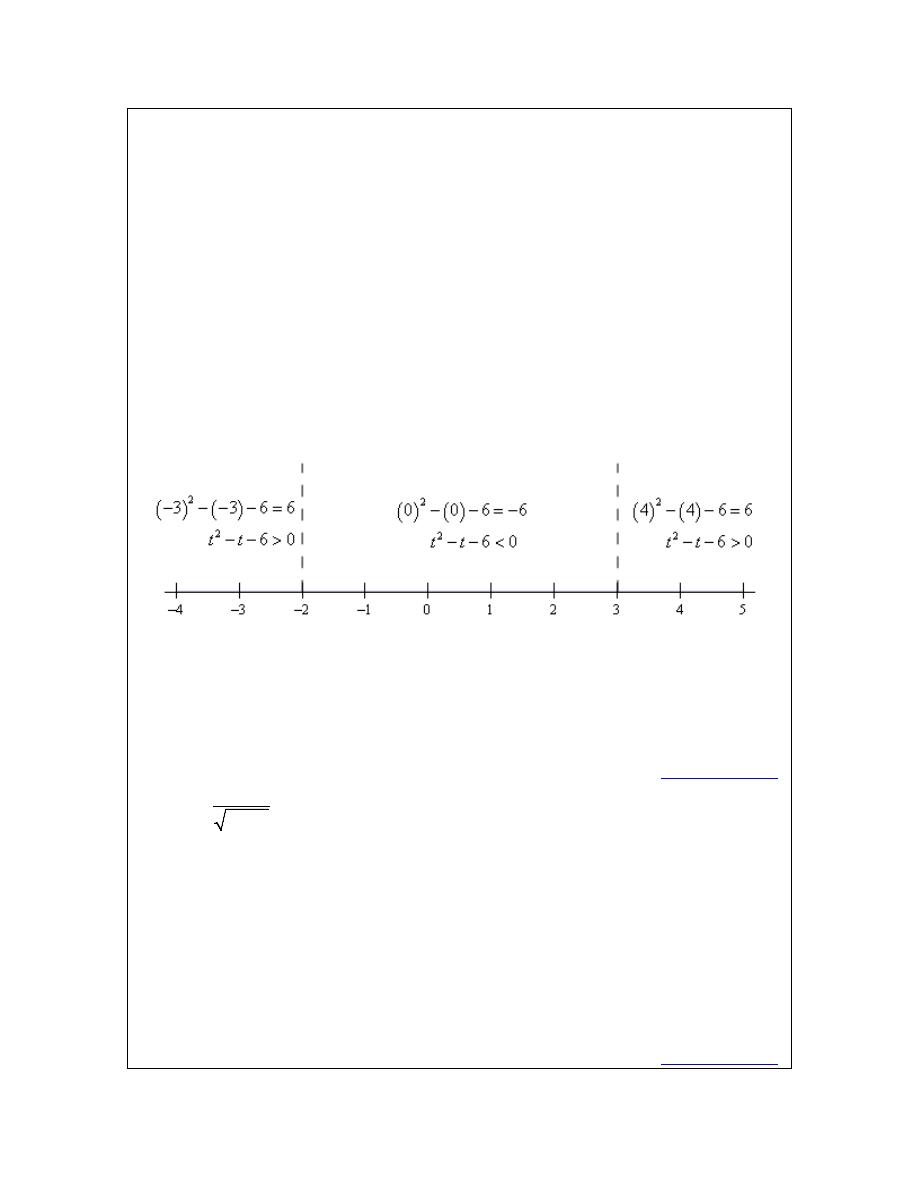
The first thing that we need to do is determine where the function is zero and that’s not too
difficult in this case.

(

)(

)

− − = −

So, the function will be zero at

= −

and

. Recall that these points will be the only place

where the function may change sign. It’s not required to change sign at these points, but these
will be the only points where the function can change sign. This means that all we need to do is
break up a number line into the three regions that avoid these two points and test the sign of the
function at a single point in each of the regions. If the function is positive at a single point in the
region it will be positive at all points in that region because it doesn’t contain the any of the
points where the function may change sign. We’ll have a similar situation if the function is
negative for the test point.

So, here is a number line showing these computations.

From this we can see that the only region in which the quadratic (in its modified form) will be
negative is in the middle region. Recalling that we got to the modified region by multiplying the
quadratic by a -1 this means that the quadratic under the root will only be positive in the middle
region and so the domain for this function is then,

[

]

Domain :

2, 3

− ≤ ≤

−

[

Return to Problems

]

(c)

( )

h x

−

In this case we have a mixture of the two previous parts. We have to worry about division by
zero and square roots of negative numbers. We can cover both issues by requiring that,

− >

Note that we need the inequality here to be strictly greater than zero to avoid the division by zero
issues. We can either solve this by the method from the previous example or, in this case, it is
easy enough to solve by inspection. The domain is this case is,

(

) (

)

Domain :

3 &

, 3 & 3,

< −

−∞ −

∞

[

Return to Problems

]

http://tutorial.math.lamar.edu/terms.aspx

Calculus I

The next topic that we need to discuss here is that of function composition. The composition of
f(x) and g(x) is

(

)( )

( )

(

)

f g x



In other words, compositions are evaluated by plugging the second function listed into the first
function listed. Note as well that order is important here. Interchanging the order will usually
result in a different answer.

Example 6

Given

( )

f x

− +

and

( )

1 20

g x

= −

find each of the following.

(a)

(

)( )



[

Solution

]

(b)

(

)( )



[

Solution

]

(c)

(

)( )



[

Solution

]

(d)

(

)( )

g g



[

Solution

]

Solution

(a)

(

)( )



In this case we’ve got a number instead of an x but it works in exactly the same way.

(

)( )

( )

(

)

(

)

29512

f g

=
=

−



[

Return to Problems

]

(b)

(

)( )



(

)( )

( )

(

)

(

)

(

) (

)

(

)

1 20

3 1 20

1 20

3 1 40

400

1 20

1200

100

f g x

=
=

−

− −

−

− +

−



Compare this answer to the next part and notice that answers are NOT the same. The order in
which the functions are listed is important!

[

Return to Problems

]

(c)

(

)( )



(

)( )

( )

(

)

(

)

(

)

1 20 3

199

g f x

− +

= −

− +

= −

−



And just to make the point. This answer is different from the previous part. Order is important in
composition.

[

Return to Problems

]

http://tutorial.math.lamar.edu/terms.aspx

Calculus I

(d)

(

)( )

g g



In this case do not get excited about the fact that it’s the same function. Composition still works
the same way.

(

)( )

( )

(

)

(

)

(

)

1 20

1 20 1 20

400

g g

g g x

=
=

−

= −

−



[

Return to Problems

]

Let’s work one more example that will lead us into the next section.

Example 7

Given

( )

f x

−

and

( )

g x

find each of the following.

(a)

(

)( )



(b)

(

)( )



Solution
(a)

(

)( )

( )

(

)

2 2

f g x

















−









= + − =



(b)

(

)( )

( )

(

)

(

)

(

)

g f x

=
=

−

− +

= − + =



In this case the two compositions were the same and in fact the answer was very simple.

(

)( ) (

)( )



This will usually not happen. However, when the two compositions are the same, or more
specifically when the two compositions are both x there is a very nice relationship between the
two functions. We will take a look at that relationship in the next section.

http://tutorial.math.lamar.edu/terms.aspx

Calculus I

Review : Inverse Functions

In the last

example

from the previous section we looked at the two functions

( )

f x

−

and

( )

g x

= +

and saw that

(

)( ) (

)( )



and as noted in that section this means that there is a nice relationship between these two
functions. Let’s see just what that relationship is. Consider the following evaluations.

( ) ( )

( )

4 2

−

= − − =

⇒

+ =

 

= + =

⇒

− = − =

 

 



−



−

In the first case we plugged

= −

into

( )

f x

and got a value of -5. We then turned around and

plugged

= −

into

( )

g x

and got a value of -1, the number that we started off with.

In the second case we did something similar. Here we plugged

into

( )

g x

and got a value

, we turned around and plugged this into

( )

f x

and got a value of 2, which is again the

number that we started with.

Note that we really are doing some function composition here. The first case is really,

(

)( )

( )

[ ]

g f

− =

−

− = −











and the second case is really,

(

)( )

( )

f g

 









 

 



Note as well that these both agree with the formula for the compositions that we found in the
previous section. We get back out of the function evaluation the number that we originally
plugged into the composition.

So, just what is going on here? In some way we can think of these two functions as undoing what

the other did to a number. In the first case we plugged

= −

into

( )

f x

and then plugged the

result from this function evaluation back into

( )

g x

and in some way

( )

g x

undid what

( )

f x

had done to

= −

and gave us back the original x that we started with.

http://tutorial.math.lamar.edu/terms.aspx

Calculus I

Function pairs that exhibit this behavior are called inverse functions. Before formally defining
inverse functions and the notation that we’re going to use for them we need to get a definition out
of the way.

A function is called one-to-one if no two values of x produce the same y. Mathematically this is
the same as saying,

( )

whenever

f x

≠

So, a function is one-to-one if whenever we plug different values into the function we get
different function values.

Sometimes it is easier to understand this definition if we see a function that isn’t one-to-one.

Let’s take a look at a function that isn’t one-to-one. The function

( )

f x

is not one-to-one

because both

( )

− =

and

( )

. In other words there are two different values of x that

produce the same value of y. Note that we can turn

( )

f x

into a one-to-one function if we

restrict ourselves to

≤ < ∞

. This can sometimes be done with functions.

Showing that a function is one-to-one is often tedious and/or difficult. For the most part we are
going to assume that the functions that we’re going to be dealing with in this course are either
one-to-one or we have restricted the domain of the function to get it to be a one-to-one function.

Now, let’s formally define just what inverse functions are. Given two one-to-one functions

( )

f x

and

( )

g x

(

)( )

(

)( )

AND



then we say that

( )

f x

and

( )

g x

are inverses of each other. More specifically we will say that

( )

g x

is the inverse of

( )

f x

and denote it by

( )

g x

−

Likewise we could also say that

( )

f x

is the inverse of

( )

g x

and denote it by

( )

f x

−

The notation that we use really depends upon the problem. In most cases either is acceptable.

For the two functions that we started off this section with we could write either of the following
two sets of notation.

( )

f x

g x

−

= +

−

http://tutorial.math.lamar.edu/terms.aspx

Calculus I

Now, be careful with the notation for inverses. The “-1” is NOT an exponent despite the fact that
is sure does look like one! When dealing with inverse functions we’ve got to remember that

( )

f x

−

≠

This is one of the more common mistakes that students make when first studying inverse
functions.

The process for finding the inverse of a function is a fairly simple one although there are a couple
of steps that can on occasion be somewhat messy. Here is the process

Finding the Inverse of a Function

Given the function

( )

f x

we want to find the inverse function,

( )

−

1. First, replace

( )

f x

with y. This is done to make the rest of the process easier.

2. Replace every x with a y and replace every y with an x.
3. Solve the equation from Step 2 for y. This is the step where mistakes are most often

made so be careful with this step.

4. Replace y with

( )

−

. In other words, we’ve managed to find the inverse at this point!

5. Verify your work by checking that

(

)

( )

−



and

(

)

( )

−



are both

true. This work can sometimes be messy making it easy to make mistakes so again be
careful.

That’s the process. Most of the steps are not all that bad but as mentioned in the process there are
a couple of steps that we really need to be careful with since it is easy to make mistakes in those
steps.

In the verification step we technically really do need to check that both

(

)

( )

−



and

(

)

( )

−



are true. For all the functions that we are going to be looking at in this course

if one is true then the other will also be true. However, there are functions (they are beyond the
scope of this course however) for which it is possible for only one of these to be true. This is
brought up because in all the problems here we will be just checking one of them. We just need
to always remember that technically we should check both.

Let’s work some examples.

Example 1

Given

( )

f x

−

find

( )

−

Solution
Now, we already know what the inverse to this function is as we’ve already done some work with
it. However, it would be nice to actually start with this since we know what we should get. This
will work as a nice verification of the process.

http://tutorial.math.lamar.edu/terms.aspx

Calculus I

So, let’s get started. We’ll first replace

( )

f x

with y.

−

Next, replace all x’s with y and all y’s with x.

−

Now, solve for y.

(

)

+ =

Finally replace y with

( )

−

( )

−

= +

Now, we need to verify the results. We already took care of this in the previous section, however,
we really should follow the process so we’ll do that here. It doesn’t matter which of the two that

we check we just need to check one of them. This time we’ll check that

(

)

( )

−



true.

(

)

( )

2 2

−





= 



















−









= + −
=



Example 2

Given

( )

g x

−

find

( )

−

Solution

The fact that we’re using

( )

g x

instead of

( )

f x

doesn’t change how the process works. Here

are the first few steps.

−

http://tutorial.math.lamar.edu/terms.aspx

Calculus I

Now, to solve for y we will need to first square both sides and then proceed as normal.

−

= −

+ =

This inverse is then,

( )

−

Finally let’s verify and this time we’ll use the other one just so we can say that we’ve gotten both
down somewhere in an example.

(

)

( )

(

)

(

)

3 3

g x

−









−

= − +
=



So, we did the work correctly and we do indeed have the inverse.

The next example can be a little messy so be careful with the work here.

Example 3

Given

( )

h x

−

find

( )

−

Solution
The first couple of steps are pretty much the same as the previous examples so here they are,

−

Now, be careful with the solution step. With this kind of problem it is very easy to make a
mistake here.

http://tutorial.math.lamar.edu/terms.aspx

Calculus I

(

)

(

)

4 5

−

= +

−

= +

− = +

−

= +

−

So, if we’ve done all of our work correctly the inverse should be,

( )

4 5

−

Finally we’ll need to do the verification. This is also a fairly messy process and it doesn’t really
matter which one we work with.

(

)

( )

4 5

h h

−





= 







= 



−





−



 −





−







Okay, this is a mess. Let’s simplify things up a little bit by multiplying the numerator and

denominator by

−

(

)

( )

(

)

(

)

(

)

(

) (

)

4 5

4 2

2 4 5

5 2

4 5

8 10

h h

−



 −





−









−





−













−









−









−



Wow. That was a lot of work, but it all worked out in the end. We did all of our work correctly
and we do in fact have the inverse.

http://tutorial.math.lamar.edu/terms.aspx

Calculus I

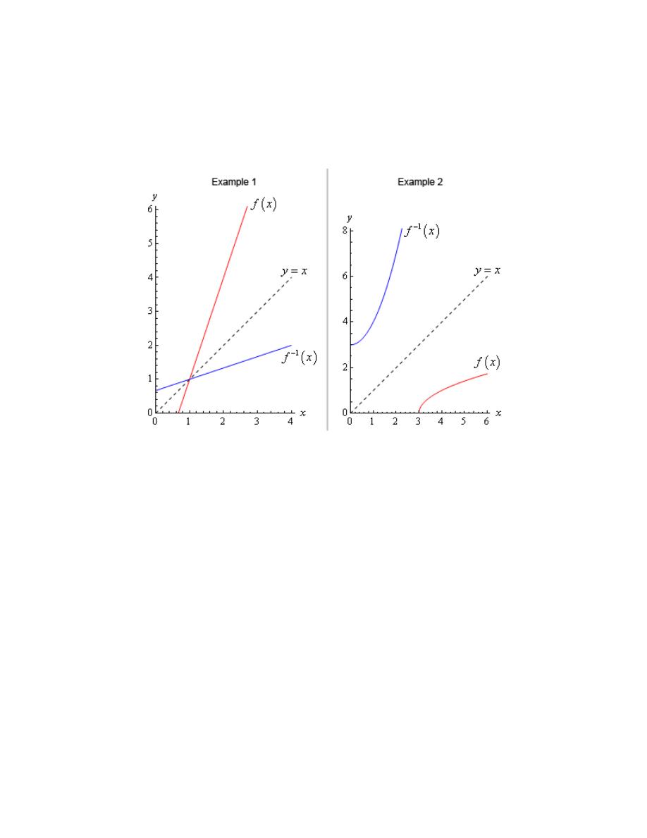
There is one final topic that we need to address quickly before we leave this section. There is an
interesting relationship between the graph of a function and the graph of its inverse.

Here is the graph of the function and inverse from the first two examples.

In both cases we can see that the graph of the inverse is a reflection of the actual function about
the line

. This will always be the case with the graphs of a function and its inverse.

http://tutorial.math.lamar.edu/terms.aspx

Calculus I

Review : Trig Functions

The intent of this section is to remind you of some of the more important (from a Calculus
standpoint…) topics from a trig class. One of the most important (but not the first) of these topics
will be how to use the unit circle. We will actually leave the most important topic to the next
section.

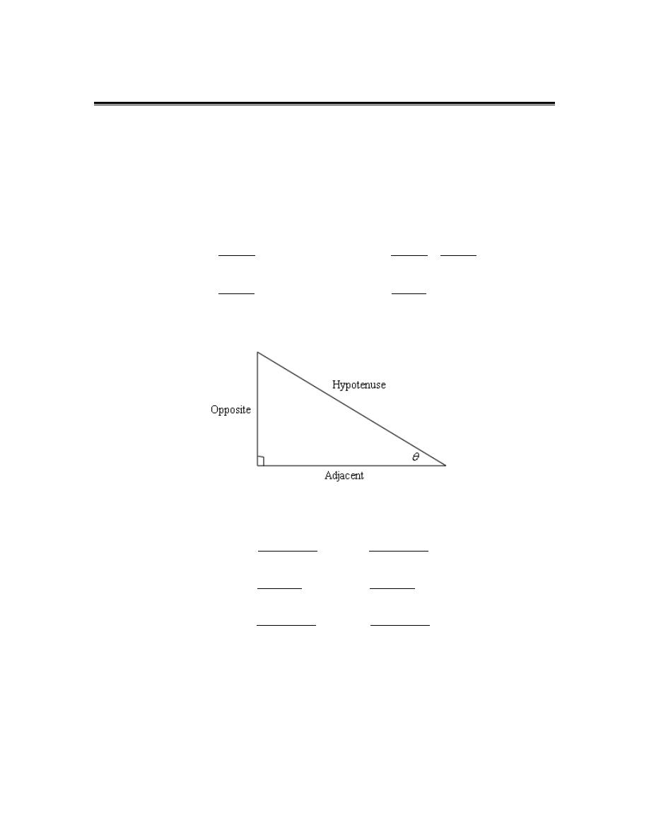
First let’s start with the six trig functions and how they relate to each other.

( )

cos

sin

cos

tan

cot

cos

sin

tan

sec

csc

cos

sin

Recall as well that all the trig functions can be defined in terms of a right triangle.

From this right triangle we get the following definitions of the six trig functions.

adjacent

cos

hypotenuse

θ =

opposite

sin

hypotenuse

θ =

opposite

tan

adjacent

θ =

adjacent

cot

opposite

θ =

hypotenuse

sec

adjacent

θ =

hypotenuse

csc

opposite

θ =

Remembering both the relationship between all six of the trig functions and their right triangle
definitions will be useful in this course on occasion.

Next, we need to touch on radians. In most trig classes instructors tend to concentrate on doing
everything in terms of degrees (probably because it’s easier to visualize degrees). The same is

http://tutorial.math.lamar.edu/terms.aspx

Calculus I

true in many science classes. However, in a calculus course almost everything is done in radians.
The following table gives some of the basic angles in both degrees and radians.

Degree 0 30

90 180 270

360

Radians 0

Know this table!  We may not see these specific angles all that much when we get into the
Calculus portion of these notes, but knowing these can help us to visualize each angle. Now, one
more time just make sure this is clear.

Be forewarned, everything in most calculus classes will be done in radians!

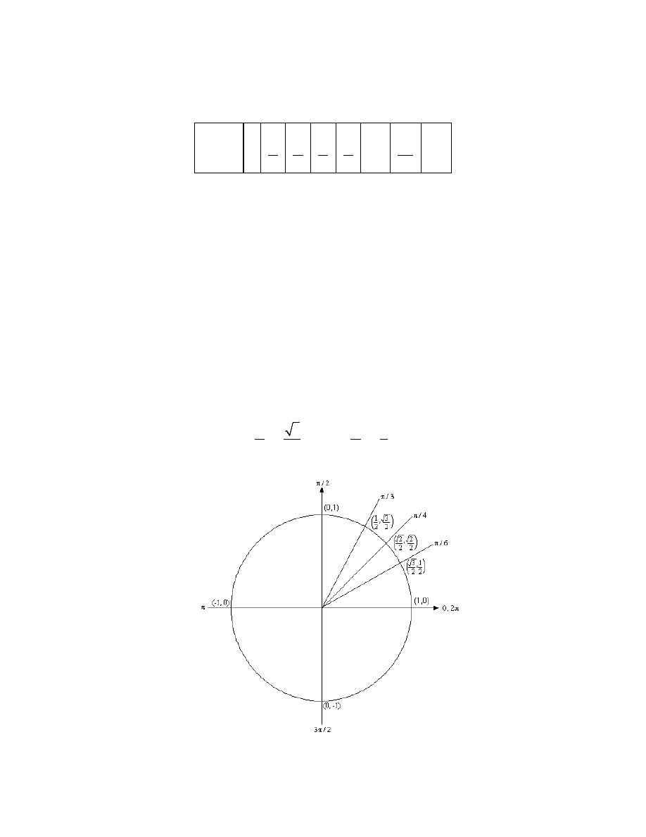
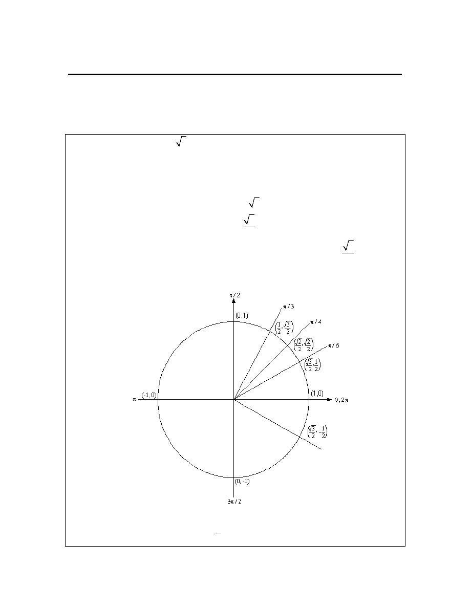
Let’s next take a look at one of the most overlooked ideas from a trig class.  The unit circle is one
of the more useful tools to come out of a trig class. Unfortunately, most people don’t learn it as
well as they should in their trig class.

Below is the unit circle with just the first quadrant filled in.  The way the unit circle works is to
draw a line from the center of the circle outwards corresponding to a given angle. Then look at
the coordinates of the point where the line and the circle intersect.  The first coordinate is the
cosine of that angle and the second coordinate is the sine of that angle. We’ve put some of the
basic angles along with the coordinates of their intersections on the unit circle. So, from the unit

circle below we can see that

cos

  =

 

 

and

sin

  =

 

 

http://tutorial.math.lamar.edu/terms.aspx

Calculus I

Remember how the signs of angles work. If you rotate in a counter clockwise direction the angle
is positive and if you rotate in a clockwise direction the angle is negative.

Recall as well that one complete revolution is

, so the positive x-axis can correspond to either

an angle of 0 or

(or

, or

−

, or

−

, etc. depending on the direction of

rotation). Likewise, the angle

(to pick an angle completely at random) can also be any of the

following angles:

(start at

then rotate once around counter clockwise)

(start at

then rotate around twice counter clockwise)

−

= −

(start at

then rotate once around clockwise)

−

= −

(start at

then rotate around twice clockwise)

etc.

In fact

can be any of the following angles

0, 1, 2, 3,

n n

= ± ± ± 

In this case n is

the number of complete revolutions you make around the unit circle starting at

. Positive

values of n correspond to counter clockwise rotations and negative values of n correspond to
clockwise rotations.

So, why did I only put in the first quadrant? The answer is simple. If you know the first quadrant
then you can get all the other quadrants from the first with a small application of geometry.
You’ll see how this is done in the following set of examples.

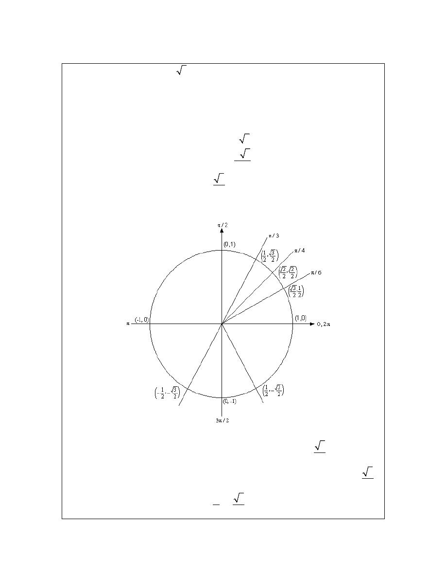
Example 1

Evaluate each of the following.

(a)

sin













and

sin





−









[

Solution

]

(b)

cos













and

cos





−









[

Solution

]

(c)

tan





−









and

tan













[

Solution

]

(d)

sec













[

Solution

]

http://tutorial.math.lamar.edu/terms.aspx

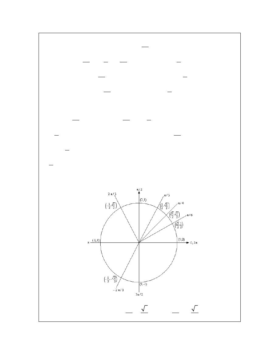
Calculus I

Solution

(a) The first evaluation in this part uses the angle

. That’s not on our unit circle above,

however notice that

= −

. So

is found by rotating up

from the negative x-axis.

This means that the line for

will be a mirror image of the line for

only in the second

quadrant. The coordinates for

will be the coordinates for

except the x coordinate will be

negative.

Likewise for

−

we can notice that

−

= − +

, so this angle can be found by rotating

down

from the negative x-axis. This means that the line for

−

will be a mirror image of

the line for

only in the third quadrant and the coordinates will be the same as the coordinates

for

except both will be negative.

Both of these angles along with their coordinates are shown on the following unit circle.

From this unit circle we can see that

sin



 =









and

sin





−

= −









http://tutorial.math.lamar.edu/terms.aspx

Calculus I

This leads to a nice fact about the sine function. The sine function is called an odd function and
so for ANY angle we have

( )

sin

− = −

[

Return to Problems

]

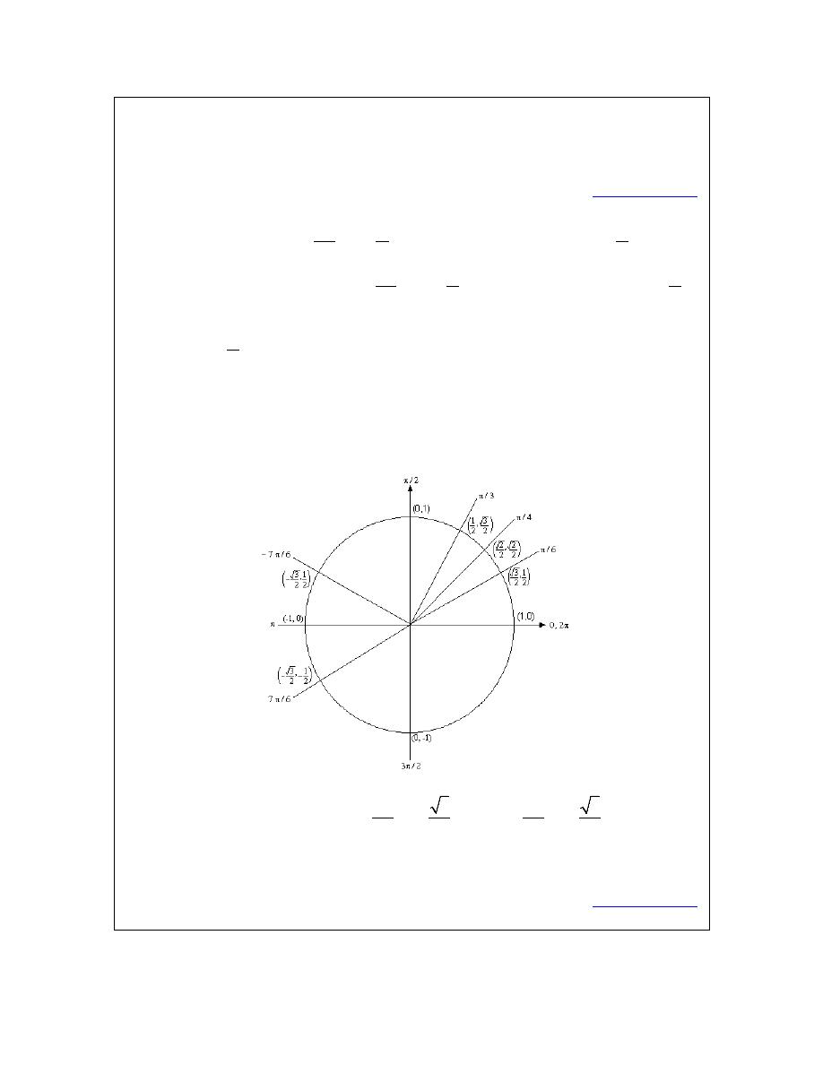
(b) For this example notice that

= +

so this means we would rotate down

from the

negative x-axis to get to this angle. Also

−

= − −

so this means we would rotate up

from the negative x-axis to get to this angle. So, as with the last part, both of these angles will be

mirror images of

in the third and second quadrants respectively and we can use this to

determine the coordinates for both of these new angles.

Both of these angles are shown on the following unit circle along with appropriate coordinates for
the intersection points.

From this unit circle we can see that

cos



 = −









and

cos





−

= −









. In this case

the cosine function is called an even function and so for ANY angle we have

( )

cos

− =

[

Return to Problems

]

http://tutorial.math.lamar.edu/terms.aspx

Calculus I

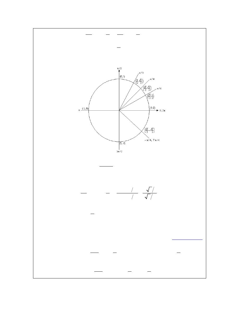
(c) Here we should note that

−

and

−

are in fact the same angle! Also

note that this angle will be the mirror image of

in the fourth quadrant. The unit circle for this

angle is

Now, if we remember that

( )

sin

tan

cos

we can use the unit circle to find the values of the

tangent function. So,

(

)

(

)

sin

2 2

tan

cos

2 2

−









−

= −









−









On a side note, notice that

tan

  =

 

 

and we can see that the tangent function is also called an

odd function and so for ANY angle we will have

( )

tan

− = −

[

Return to Problems

]

(d) Here we need to notice that

. In other words, we’ve started at

and rotated

around twice to end back up at the same point on the unit circle. This means that

sec

sec 4

sec









 









 









 

http://tutorial.math.lamar.edu/terms.aspx

Calculus I

Now, let’s also not get excited about the secant here. Just recall that

( )

sec

cos

and so all we need to do here is evaluate a cosine! Therefore,

sec

cos





 





 

 





 

 

 

[

Return to Problems

]

So, in the last example we saw how the unit circle can be used to determine the value of the trig
functions at any of the “common” angles. It’s important to notice that all of these examples used
the fact that if you know the first quadrant of the unit circle and can relate all the other angles to
“mirror images” of one of the first quadrant angles you don’t really need to know whole unit
circle. If you’d like to see a complete unit circle I’ve got one on my

Trig Cheat Sheet

that is

available at

http://tutorial.math.lamar.edu

Another important idea from the last example is that when it comes to evaluating trig functions all
that you really need to know is how to evaluate sine and cosine. The other four trig functions are
defined in terms of these two so if you know how to evaluate sine and cosine you can also
evaluate the remaining four trig functions.

We’ve not covered many of the topics from a trig class in this section, but we did cover some of
the more important ones from a calculus standpoint. There are many important trig formulas that
you will use occasionally in a calculus class. Most notably are the half-angle and double-angle
formulas. If you need reminded of what these are, you might want to download my

Trig Cheat

Sheet

as most of the important facts and formulas from a trig class are listed there.

http://tutorial.math.lamar.edu/terms.aspx

Calculus I

Review : Solving Trig Equations

In this section we will take a look at solving trig equations. This is something that you will be
asked to do on a fairly regular basis in my class.

Let’s just jump into the examples and see how to solve trig equations.

Example 1

Solve

( )

2 cos

Solution
There’s really not a whole lot to do in solving this kind of trig equation. All we need to do is
divide both sides by 2 and the go to the unit circle.

( )

2 cos

cos

So, we are looking for all the values of t for which cosine will have the value of

. So, let’s

take a look at the following unit circle.

From quick inspection we can see that

is a solution. However, as I have shown on the unit

http://tutorial.math.lamar.edu/terms.aspx

Calculus I

circle there is another angle which will also be a solution. We need to determine what this angle

is. When we look for these angles we typically want positive angles that lie between 0 and

This angle will not be the only possibility of course, but by convention we typically look for
angles that meet these conditions.

To find this angle for this problem all we need to do is use a little geometry. The angle in the first

quadrant makes an angle of

with the positive x-axis, then so must the angle in the fourth

quadrant. So we could use

−

, but again, it’s more common to use positive angles so, we’ll use

− =

We aren’t done with this problem. As the discussion about finding the second angle has shown

there are many ways to write any given angle on the unit circle. Sometimes it will be

−

that

we want for the solution and sometimes we will want both (or neither) of the listed angles.
Therefore, since there isn’t anything in this problem (contrast this with the next problem) to tell
us which is the correct solution we will need to list ALL possible solutions.

This is very easy to do. Recall from the previous

section

and you’ll see there that I used

0, 1, 2, 3,

n n

= ± ± ± 

to represent all the possible angles that can end at the same location on the unit circle, i.e. angles

that end at

. Remember that all this says is that we start at

then rotate around in the

counter-clockwise direction (n is positive) or clockwise direction (n is negative) for n complete
rotations. The same thing can be done for the second solution.

So, all together the complete solution to this problem is

0, 1, 2, 3,

n n

= ± ± ±



As a final thought, notice that we can get

−

by using

= −

in the second solution.

Now, in a calculus class this is not a typical trig equation that we’ll be asked to solve. A more
typical example is the next one.

http://tutorial.math.lamar.edu/terms.aspx

Calculus I

Example 2

Solve

( )

2 cos

[ 2 , 2 ]

π π

−

Solution
In a calculus class we are often more interested in only the solutions to a trig equation that fall in
a certain interval. The first step in this kind of problem is to first find all possible solutions. We
did this in the first example.

0, 1, 2, 3,

n n

= ± ± ±



Now, to find the solutions in the interval all we need to do is start picking values of n, plugging
them in and getting the solutions that will fall into the interval that we’ve been given.

n=0.

( )

Now, notice that if we take any positive value of n we will be adding on positive multiples of 2

onto a positive quantity and this will take us past the upper bound of our interval and so we don’t
need to take any positive value of n.

However, just because we aren’t going to take any positive value of n doesn’t mean that we
shouldn’t also look at negative values of n.

n=-1.

( )

− = −

> −

− = − > −

These are both greater than

−

and so are solutions, but if we subtract another

off (i.e use

= −

) we will once again be outside of the interval so we’ve found all the possible solutions

that lie inside the interval

[ 2 , 2 ]

π π

−

So, the solutions are :

−

So, let’s see if you’ve got all this down.

http://tutorial.math.lamar.edu/terms.aspx

Calculus I

Example 3

Solve

( )

2 sin 5

= −

[

, 2 ]

π π

−

Solution
This problem is very similar to the other problems in this section with a very important
difference. We’ll start this problem in exactly the same way. We first need to find all possible
solutions.

2 sin(5 )

sin(5 )

= −

−

So, we are looking for angles that will give

−

out of the sine function. Let’s again go to our

trusty unit circle.

Now, there are no angles in the first quadrant for which sine has a value of

−

. However,

there are two angles in the lower half of the unit circle for which sine will have a value of

−

So, what are these angles? We’ll notice

sin

  =

 

 

, so the angle in the third quadrant will be

http://tutorial.math.lamar.edu/terms.aspx

Calculus I

below the negative x-axis or

+ =

. Likewise, the angle in the fourth quadrant will

below the positive x-axis or

− =

. Remember that we’re typically looking for positive

angles between 0 and

Now we come to the very important difference between this problem and the previous problems
in this section. The solution is NOT

0, 1, 2,

= ± ±



This is not the set of solutions because we are NOT looking for values of x for which

( )

sin

= −

, but instead we are looking for values of x for which

( )

sin 5

= −

. Note the

difference in the arguments of the sine function! One is x and the other is

. This makes all the

difference in the world in finding the solution! Therefore, the set of solutions is

0, 1, 2,

= ± ±



Well, actually, that’s not quite the solution. We are looking for values of x so divide everything
by 5 to get.

0, 1, 2,

= ± ±

= +

= ± ±



Notice that we also divided the

2 n

by 5 as well! This is important! If we don’t do that you

WILL miss solutions. For instance, take

sin 5

sin

sin 5

sin













⇒

= −





































= +

⇒

= −

























I’ll leave it to you to verify my work showing they are solutions. However it makes the point. If

you didn’t divided the

2 n

by 5 you would have missed these solutions!

Okay, now that we’ve gotten all possible solutions it’s time to find the solutions on the given
interval. We’ll do this as we did in the previous problem. Pick values of n and get the solutions.

http://tutorial.math.lamar.edu/terms.aspx

Calculus I

n = 0.

( )

= +

n = 1.

( )

= +

n = 2.

( )

= +

n = 3.

( )

= +

n = 4.

( )

= +

n = 5.

( )

= +

Okay, so we finally got past the right endpoint of our interval so we don’t need any more positive
n. Now let’s take a look at the negative n and see what we’ve got.

n = –1 .

( )

−

= −

> −

−

= +

= −

> −

http://tutorial.math.lamar.edu/terms.aspx

Calculus I

n = –2.

( )

−

= −

> −

−

= +

= −

> −

n = –3.

( )

−

= −

> −

−

= +

= −

> −

n = –4.

( )

−

= −

< −

−

= +

= −

< −

And we’re now past the left endpoint of the interval. Sometimes, there will be many solutions as
there were in this example. Putting all of this together gives the following set of solutions that lie
in the given interval.

15 3

π π π

−

Let’s work another example.

Example 4

Solve

( )

sin 2

cos 2

= −

π π





−









Solution
This problem is a little different from the previous ones. First, we need to do some rearranging
and simplification.

( )

sin(2 )

cos(2 )

sin(2 )

cos(2 )

tan 2

= −

So, solving

sin(2 )

cos(2 )

= −

is the same as solving

tan(2 )

= −

. At some level we didn’t

need to do this for this problem as all we’re looking for is angles in which sine and cosine have
the same value, but opposite signs. However, for other problems this won’t be the case and we’ll
want to convert to tangent.

http://tutorial.math.lamar.edu/terms.aspx

Calculus I

Looking at our trusty unit circle it appears that the solutions will be,

0, 1, 2,

= ± ±



Or, upon dividing by the 2 we get all possible solutions.

0, 1, 2,

π π

= ± ±



Now, let’s determine the solutions that lie in the given interval.

n = 0.

( )

n = 1.

( )

Unlike the previous example only one of these will be in the interval. This will happen
occasionally so don’t always expect both answers from a particular n to work. Also, we should
now check n=2 for the first to see if it will be in or out of the interval. I’ll leave it to you to check
that it’s out of the interval.

Now, let’s check the negative n.

n = –1.

( )

− = −

> −

− = − > −

n = –2.

( )

− = −

< −

− = −

> −

Again, only one will work here. I’ll leave it to you to verify that n = –3 will give two answers

http://tutorial.math.lamar.edu/terms.aspx

Calculus I

that are both out of the interval.

The complete list of solutions is then,

π π π

−

Let’s work one more example so that I can make a point that needs to be understood when
solving some trig equations.

Example 5

Solve

( )

cos 3

Solution
This example is designed to remind you of certain properties about sine and cosine. Recall that

( )

1 cos

− ≤

≤

and

( )

1 sin

− ≤

≤

. Therefore, since cosine will never be greater that 1 it

definitely can’t be 2. So THERE ARE NO SOLUTIONS to this equation!

It is important to remember that not all trig equations will have solutions.

In this section we solved some simple trig equations. There are more complicated trig equations
that we can solve so don’t leave this section with the feeling that there is nothing harder out there
in the world to solve. In fact, we’ll see at least one of the more complicated problems in the next
section. Also, every one of these problems came down to solutions involving one of the
“common” or “standard” angles. Most trig equations won’t come down to one of those and will
in fact need a calculator to solve. The next section is devoted to this kind of problem.

http://tutorial.math.lamar.edu/terms.aspx

Calculus I

Review : Solving Trig Equations with Calculators, Part I

In the previous section we started solving trig equations. The only problem with the equations we
solved in there is that they pretty much all had solutions that came from a handful of “standard”
angles and of course there are many equations out there that simply don’t. So, in this section we
are going to take a look at some more trig equations, the majority of which will require the use of
a calculator to solve (a couple won’t need a calculator).

The fact that we are using calculators in this section does not however mean that the problems in
the previous section aren’t important. It is going to be assumed in this section that the basic ideas
of solving trig equations are known and that we don’t need to go back over them here. In
particular, it is assumed that you can use a unit circle to help you find all answers to the equation
(although the process here is a little different as we’ll see) and it is assumed that you can find
answers in a given interval. If you are unfamiliar with these ideas you should first go to the
previous section and go over those problems.

Before proceeding with the problems we need to go over how our calculators work so that we can
get the correct answers. Calculators are great tools but if you don’t know how they work and
how to interpret their answers you can get in serious trouble.

First, as already pointed out in previous sections, everything we are going to be doing here will be
in radians so make sure that your calculator is set to radians before attempting the problems in
this section. Also, we are going to use 4 decimal places of accuracy in the work here. You can
use more if you want, but in this class we’ll always use at least 4 decimal places of accuracy.

Next, and somewhat more importantly, we need to understand how calculators give answers to
inverse trig functions. We didn’t cover inverse trig functions in this review, but they are just
inverse functions and we have talked a little bit about inverse functions in a review

section

. The

only real difference is that we are now using trig functions. We’ll only be looking at three of
them and they are:

( )

Inverse Cosine : cos

arccos

Inverse Sine : sin

arcsin

Inverse Tangent : tan

arctan

−

As shown there are two different notations that are commonly used.  In these notes we’ll be using
the first form since it is a little more compact. Most calculators these days will have buttons on
them for these three so make sure that yours does as well.

We now need to deal with how calculators give answers to these.  Let’s suppose, for example,

that we wanted our calculator to compute

( )

3
4

cos

−

. First, remember that what the calculator is

actually computing is the angle, let’s say x, that we would plug into cosine to get a value of

3
4

, or

http://tutorial.math.lamar.edu/terms.aspx

Calculus I

( )

cos

−

 

⇒

 

 

So, in other words, when we are using our calculator to compute an inverse trig function we are
really solving a simple trig equation.

Having our calculator compute

( )

3
4

cos

−

and hence solve

( )

3
4

cos x

gives,

cos

0.7227

−

 

 

 

From the previous section we know that there should in fact be an infinite number of answers to

this including a second angle that is in the interval

[

]

0, 2

. However, our calculator only gave us

a single answer. How to determine what the other angles are will be covered in the following
examples so we won’t go into detail here about that. We did need to point out however, that the
calculators will only give a single answer and that we’re going to have more work to do than just
plugging a number into a calculator.

Since we know that there are supposed to be an infinite number of solutions to

( )

3
4

cos x

the

next question we should ask then is just how did the calculator decide to return the answer that it
did? Why this one and not one of the others? Will it give the same answer every time?

There are rules that determine just what answer the calculator gives. All calculators will give
answers in the following ranges.

( )

cos

sin

tan

−

≤

− ≤

≤

− <

If you think back to the unit circle and recall that we think of cosine as the horizontal axis then we
can see that we’ll cover all possible values of cosine in the upper half of the circle and this is
exactly the range given above for the inverse cosine. Likewise, since we think of sine as the
vertical axis in the unit circle we can see that we’ll cover all possible values of sine in the right
half of the unit circle and that is the range given above.

For the tangent range look back to the graph of the tangent function itself and we’ll see that one
branch of the tangent is covered in the range given above and so that is the range we’ll use for
inverse tangent. Note as well that we don’t include the endpoints in the range for inverse tangent
since tangent does not exist there.

So, if we can remember these rules we will be able to determine the remaining angle in

[

]

0, 2

that also works for each solution.

http://tutorial.math.lamar.edu/terms.aspx

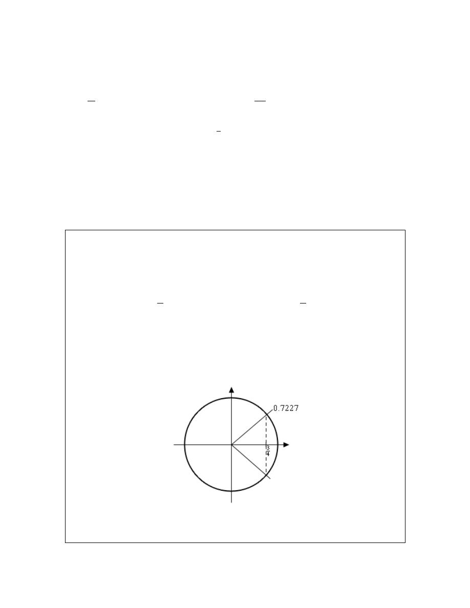
Calculus I

As a final quick topic let’s note that it will, on occasion, be useful to remember the decimal
representations of some basic angles. So here they are,

1.5708

3.1416

4.7124

6.2832

Using these we can quickly see that

( )

3
4

cos

−

must be in the first quadrant since 0.7227 is

between 0 and 1.5708. This will be of great help when we go to determine the remaining angles

So, once again, we can’t stress enough that calculators are great tools that can be of tremendous
help to us, but it you don’t understand how they work you will often get the answers to problems
wrong.

So, with all that out of the way let’s take a look at our first problem.

Example 1

Solve

( )

4 cos

on[-8,10].

Solution
Okay, the first step here is identical to the problems in the previous section. We first need to
isolate the cosine on one side by itself and then use our calculator to get the first answer.

( )

cos

0.7227

−

 

⇒

 

 

So, this is the one we were using above in the opening discussion of this section. At the time we
mentioned that there were infinite number of answers and that we’d be seeing how to find them
later. Well that time is now.

First, let’s take a quick look at a unit circle for this example.

The angle that we’ve found is shown on the circle as well as the other angle that we know should
also be an answer. Finding this angle here is just as easy as in the previous section. Since the

http://tutorial.math.lamar.edu/terms.aspx

Calculus I

line segment in the first quadrant forms an angle of 0.7227 radians with the positive x-axis then so
does the line segment in the fourth quadrant. This means that we can use either -0.7227 as the

second angle or

0.7227

5.5605

−

. Which you use depends on which you prefer. We’ll

pretty much always use the positive angle to avoid the possibility that we’ll lose the minus sign.

So, all possible solutions, ignoring the interval for a second, are then,

0.7227

0, 1, 2,

5.5605 2

= ± ±



Now, all we need to do is plug in values of n to determine the angle that are actually in the
interval. Here’s the work for that.

2 :

11.8437

= −

and

7.0059

1 :

5.5605

and

0.7227

and

5.5605

7.0059

and

11.8437

−

= −

−

So, the solutions to this equation, in the given interval, are,

7.0059,

5.5605,

0.7227, 0.7227, 5.5605, 7.0059

= −

−

Note that we had a choice of angles to use for the second angle in the previous example. The
choice of angles there will also affect the value(s) of n that we’ll need to use to get all the
solutions. In the end, regardless of the angle chosen, we’ll get the same list of solutions, but the
value(s) of n that give the solutions will be different depending on our choice.

Also, in the above example we put in a little more explanation than we’ll show in the remaining
examples in this section to remind you how these work.

Example 2

Solve

( )

10 cos 3

−

on [-2,5].

Solution
Okay, let’s first get the inverse cosine portion of this problem taken care of.

( )

cos 3

cos

2.3462

−





= −

⇒

−









Don’t forget that we still need the “3”!

Now, let’s look at a quick unit circle for this problem. As we can see the angle 2.3462 radians is
in the second quadrant and the other angle that we need is in the third quadrant.  We can find this
second angle in exactly the same way we did in the previous example.  We can use either -2.3462

http://tutorial.math.lamar.edu/terms.aspx

Calculus I

or we can use

2.3462

3.9370

−

. As with the previous example we’ll use the positive

choice, but that is purely a matter of preference. You could use the negative if you wanted to.

So, let’s now finish out the problem. First, let’s acknowledge that the values of 3t that we need
are,

2.3462 2

0, 1, 2,

3.9370 2

= ± ±



Now, we need to properly deal with the 3, so divide that out to get all the solutions to the trig
equation.

0.7821

0, 1, 2,

1.3123

= ± ±



Finally, we need to get the values in the given interval.

2 :

3.4067

= −

and

2.8765

−

1 :

1.3123

and

0.7821

and

1.3123

2.8765

and

3.4067

2 :

4.9709

and

5.5011

= −

−

The solutions to this equation, in the given interval are then,

1.3123,

0.7821, 0.7821, 1.3123, 2.8765, 3.4067, 4.9709

= −

−

We’ve done a couple of basic problems with cosines, now let’s take a look at how solving
equations with sines work.

http://tutorial.math.lamar.edu/terms.aspx

Calculus I

Example 3

Solve

6 sin

  =

 

 

on [-20,30]

Solution
Let’s first get the calculator work out of the way since that isn’t where the difference comes into
play.

sin

0.1674

−

 

⇒

 

 

Here’s a unit circle for this example.

To find the second angle in this case we can notice that the line in the first quadrant makes an
angle of 0.1674 with the positive x-axis and so the angle in the second quadrant will then make an
angle of 0.1674 with the negative x-axis and so the angle that we’re after is then,

0.1674

2.9742

−

Here’s the rest of the solution for this example. We’re going to assume from this point on that
you can do this work without much explanation.

0.1674 2

0.3348 4

0, 1, 2,

5.9484 4

2.9742 2

π
π

⇒

= ± ±



2 :

24.7980

= −

and

19.1844

1 :

12.2316

and

6.6180

0.3348

and

5.9484

12.9012

and

18.5148

25.4676

and

31.0812

−

= −

−

The solutions to this equation are then,

19.1844,

12.2316,

6.6180, 0.3348, 5.9484, 12.9012, 18.5128, 25.4676

= −

−

http://tutorial.math.lamar.edu/terms.aspx

Calculus I

Example 4

Solve

( )

3sin 5

= −

on [0,1].

Solution
You should be getting pretty good at these by now, so we won’t be putting much explanation in
for this one. Here we go.

( )

sin 5

sin

0.7297

−





= −

⇒

−

= −









Okay, with this one we’re going to do a little more work than with the others. For the first angle
we could use the answer our calculator gave us. However, it’s easy to lose minus signs so we’ll

instead use

0.7297

5.5535

−

. Again, there is no reason to this other than a worry about

losing the minus sign in the calculator answer. If you’d like to use the calculator answer you are
more than welcome to. For the second angle we’ll note that the lines in the third and fourth
quadrant make an angle of 0.7297 with the x-axis and so the second angle is

0.7297

3.8713

Here’s the rest of the work for this example.

1.1107

5.5535 2

0, 1, 2,

3.8713 2

0.7743

π
π

⇒

= ± ±



1 :

0.1460

= −

and

0.4823

−

1.1107

and

0.7743

So, in this case we get a single solution of 0.7743.

Note that in the previous example we only got a single solution. This happens on occasion so
don’t get worried about it. Also, note that it was the second angle that gave this solution and so if

http://tutorial.math.lamar.edu/terms.aspx

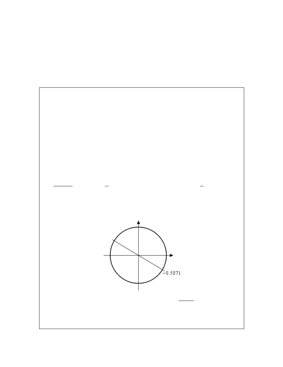
Calculus I

we’d just relied on our calculator without worrying about other angles we would not have gotten
this solution. Again, it can’t be stressed enough that while calculators are a great tool if we don’t
understand how to correctly interpret/use the result we can (and often will) get the solution
wrong.

To this point we’ve only worked examples involving sine and cosine. Let’s now work a couple
of examples that involve other trig functions to see how they work.

Example 5

Solve

( )

9 sin 2

5 cos 2

= −

on[-10,0].

Solution
At first glance this problem seems to be at odds with the sentence preceding the example.
However, it really isn’t.

First, when we have more than one trig function in an equation we need a way to get equations
that only involve one trig function. There are many ways of doing this that depend on the type of
equation we’re starting with. In this case we can simply divide both sides by a cosine and we’ll
get a single tangent in the equation. We can now see that this really is an equation that doesn’t
involve a sine or a cosine.

So, let’s get started on this example.

( )

sin 2

tan 2

tan

0.5071

cos 2

−





= −

⇒

−

= −









Now, the unit circle doesn’t involve tangents, however we can use it to illustrate the second angle

in the range

[

]

0, 2

The angles that we’re looking for here are those whose quotient of

sine

cosine

is the same. The

second angle where we will get the same value of tangent will be exactly opposite of the given
point. For this angle the values of sine and cosine are the same except they will have opposite
signs. In the quotient however, the difference in signs will cancel out and we’ll get the same

http://tutorial.math.lamar.edu/terms.aspx

Calculus I

value of tangent. So, the second angle will always be the first angle plus

Before getting the second angle let’s also note that, like the previous example, we’ll use the

0.5071 5.7761

−

for the first angle. Again, this is only because of a concern about losing

track of the minus sign in our calculator answer. We could just as easily do the work with the
original angle our calculator gave us.

Now, this is where is seems like we’re just randomly making changes and doing things for no
reason. The second angle that we’re going to use is,

(

)

0.5071

2.6345

+ −

= −

The fact that we used the calculator answer here seems to contradict the fact that we used a
different angle for the first above. The reason for doing this here is to give a second angle that is

in the range

[

]

0, 2

. Had we used 5.7761 to find the second angle we’d get

5.7761 8.9177

. This is a perfectly acceptable answer, however it is larger than

(6.2832) and the general rule of thumb is to keep the initial angles as small as possible.

Here are all the solutions to the equation.

5.7761 2

2.8881

0, 1, 2,

2.6345 2

1.3173

⇒

= ± ±



4 :

9.6783

and

11.2491

= −

−

3 :

6.5367

and

8.1075

2 :

3.3951

and

4.9659

1 :

0.2535

and

1.8243

2.8881

= −

−

= −

−

= −

−

and

1.3173

The seven solutions to this equation are then,

0.2535,

1.8243,

3.3951,

4.9659,

6.5367,

8.1075,

9.6783

−

Note as well that we didn’t need to do the

and computation since we could see from the

given interval that we only wanted negative answers and these would clearly give positive
answers.

Most calculators today can only do inverse sine, inverse cosine, and inverse tangent. So, let’s see
an example that uses one of the other trig functions.

http://tutorial.math.lamar.edu/terms.aspx

Calculus I

Example 6

Solve

( )

7 sec 3

= −

Solution
We’ll start this one in exactly the same way we’ve done all the others.

( )

sec 3

sec

−





= −

⇒

−









Now we reach the problem. As noted above, most calculators can’t handle inverse secant so
we’re going to need a different solution method for this one. To finish the solution here we’ll
simply recall the definition of secant in terms of cosine and convert this into an equation
involving cosine instead and we already know how to solve those kinds of trig equations.

( )

sec 3

cos 3

= −

⇒

= −

Now, we solved this equation in the second example above so we won’t redo our work here. The
solution is,

0.7821

0, 1, 2,

1.3123

= ± ±



We weren’t given an interval in this problem so here is nothing else to do here.

For the remainder of the examples in this section we’re not going to be finding solutions in an
interval to save some space. If you followed the work from the first few examples in which we
were given intervals you should be able to do any of the remaining examples if given an interval.

Also, we will no longer be including sketches of unit circles in the remaining solutions. We are
going to assume that you can use the above sketches as guides for sketching unit circles to verify
our claims in the following examples.

The next three examples don’t require a calculator but are important enough or cause enough
problems for students to include in this section in case you run across them and haven’t seen them
anywhere else.

http://tutorial.math.lamar.edu/terms.aspx

Calculus I

Example 7

Solve

( )

cos 4

θ = −

Solution
There really isn’t too much to do with this problem. It is, however, different from all the others

done to this point. All the others done to this point have had two angles in the interval

[

]

0, 2

that were solutions to the equation. This only has one. Here is the solution to this equation.

0, 1, 2,

π π

θ π

= +

⇒

= +

= ± ± 

Example 8

Solve

sin

  =

 

 

Solution
Again, not much to this problem. Using a unit circle it isn’t too hard to see that the solutions to
this equation are,

0 2

0, 1, 2,

= +

⇒

= ± ±

= +



This next example has an important point that needs to be understood when solving some trig
equations.

Example 9

Solve

( )

sin 3

Solution
This example is designed to remind you of certain properties about sine and cosine. Recall that

( )

1 sin

− ≤

≤

and

( )

1 cos

− ≤

≤

. Therefore, since sine will never be greater that 1 it

definitely can’t be 2. So THERE ARE NO SOLUTIONS to this equation!

It is important to remember that not all trig equations will have solutions.

Because this document is also being prepared for viewing on the web we’re going to split this
section in two in order to keep the page size (and hence load time in a browser) to a minimum. In
the next section we’re going to take a look at some slightly more “complicated” equations.
Although, as you’ll see, they aren’t as complicated as they may at first seem.

http://tutorial.math.lamar.edu/terms.aspx

Calculus I

Review : Solving Trig Equations with Calculators, Part II

Because this document is also being prepared for viewing on the web we split this section into
two parts to keep the size of the pages to a minimum.

Also, as with the last few examples in the previous part of this section we are not going to be
looking for solutions in an interval in order to save space. The important part of these examples
is to find the solutions to the equation. If we’d been given an interval it would be easy enough to
find the solutions that actually fall in the interval.

In all the examples in the previous section all the arguments, the

, etc., were fairly simple.

Let’s take a look at an example that has a slightly more complicated argument.

Example 1

Solve

(

)

5 cos 2

− = −

Solution
Note that the argument here is not really all that complicated but the addition of the “-1” often
seems to confuse people so we need to a quick example with this kind of argument. The solution
process is identical to all the problems we’ve done to this point so we won’t be putting in much
explanation. Here is the solution.

(

)

cos 2

cos

2.2143

−





− = −

⇒

− =

−









This angle is in the second quadrant and so we can use either -2.2143 or

2.2143

4.0689

−

for the second angle. As usual for these notes we’ll use the positive one. Therefore the two
angles are,

2.2143 2

0, 1, 2,

4.0689 2

− =

= ± ±

− =



Now, we still need to find the actual values of x that are the solutions. These are found in the
same manner as all the problems above. We’ll first add 1 to both sides and then divide by 2.
Doing this gives,

1.6072

0, 1, 2,

2.5345

= ± ±



So, in this example we saw an argument that was a little different from those seen previously, but
not all that different when it comes to working the problems so don’t get too excited about it.

http://tutorial.math.lamar.edu/terms.aspx

Calculus I

We now need to move into a different type of trig equation. All of the trig equations solved to
this point (the previous example as well as the previous section) were, in some way, more or less
the “standard” trig equation that is usually solved in a trig class. There are other types of
equations involving trig functions however that we need to take a quick look at. The remaining
examples show some of these different kinds of trig equations.

Example 2

Solve

( )

( ) ( )

2 cos 6

11cos 6

sin 3

Solution
So, this definitely doesn’t look like any of the equations we’ve solved to this point and initially

the process is different as well. First, notice that there is a

( )

cos 6 y

in each term, so let’s factor

that out and see what we have.

( )

(

)

cos 6

2 11sin 3

We now have a product of two terms that is zero and so we know that we must have,

( )

cos 6

2 11sin 3

Now, at this point we have two trig equations to solve and each is identical to the type of equation
we were solving earlier. Because of this we won’t put in much detail about solving these two
equations.

First, solving

( )

cos 6

gives,

0, 1, 2,

π π

= +

⇒

= ± ±

= +



Next, solving

( )

2 11sin 3

gives,

2.0335

6.1004 2

0, 1, 2,

3.3244 2

1.1081

π
π

⇒

= ± ±



Remember that in these notes we tend to take positive angles and so the first solution here is in

fact

0.1828

−

where our calculator gave us -0.1828 as the answer when using the inverse

sine function.

The solutions to this equation are then,

http://tutorial.math.lamar.edu/terms.aspx

Calculus I

0, 1, 2,

2.0335

1.1081

π π

= +

= ± ±



This next example also involves “factoring” trig equations but in a slightly different manner than
the previous example.

Example 3

Solve

4 sin

3sin

 

−

 

 

Solution
Before solving this equation let’s solve an apparently unrelated equation.

(

)(

)

−

⇒

−

− =

⇒

= −

This is an easy (or at least I hope it’s easy as this point) equation to solve. The obvious question
then is, why did we do this? We’ll, if you compare the two equations you’ll see that the only real
difference is that the one we just solved has an x everywhere and the equation we want to solve
has a sine. What this tells us is that we can work the two equations in exactly the same way.

We, will first “factor” the equation as follows,

4 sin

3sin

4 sin

sin







 

−

− =

 







 







Now, set each of the two factors equal to zero and solve for the sine,

sin

 

= −

 

 

We now have two trig equations that we can easily (hopefully…) solve at this point. We’ll leave
the details to you to verify that the solutions to each of these and hence the solutions to the
original equation are,

18.0915 6

10.1829 6

0, 1, 2,

π
π

= ± ±



The first two solutions are from the first equation and the third solution is from the second
equation.

http://tutorial.math.lamar.edu/terms.aspx

Calculus I

Let’s work one more trig equation that involves solving a quadratic equation. However, this time,
unlike the previous example this one won’t factor and so we’ll need to use the quadratic formula.

Example 4

Solve

(

)

(

)

8 cos 1

13cos 1

− +

− − =

Solution
Now, as mentioned prior to starting the example this quadratic does not factor. However, that
doesn’t mean all is lost. We can solve the following equation with the quadratic formula (you do

remember

this and how to use it right?),

329

0.3211,

1.9461

− ±

− =

⇒

−

So, if we can use the quadratic formula on this then we can also use it on the equation we’re
asked to solve. Doing this gives us,

(

)

(

)

cos 1

0.3211

cos 1

1.9461

−

= −

Now, recall

Example 9

from the previous section. In that example we noted that

( )

1 cos

− ≤

≤

and so the second equation will have no solutions. Therefore, the solutions to

the first equation will yield the only solutions to our original equation. Solving this gives the
following set of solutions,

0.2439 2

0, 1, 2,

4.0393 2

= −

−

= ± ±

= −

−



Note that we did get some negative numbers here and that does seem to violate the general form
that we’ve been using in most of these examples. However, in this case the “-” are coming about
when we solved for x after computing the inverse cosine in our calculator.

There is one more example in this section that we need to work that illustrates another way in
which factoring can arise in solving trig equations. This equation is also the only one where the
variable appears both inside and outside of the trig equation. Not all equations in this form can be
easily solved, however some can so we want to do a quick example of one.

http://tutorial.math.lamar.edu/terms.aspx

Calculus I

Example 5

Solve

( )

5 tan 8

Solution
First, before we even start solving we need to make one thing clear. DO NOT CANCEL AN x
FROM BOTH SIDES!!! While this may seem like a natural thing to do it WILL cause us to
lose a solution here.

So, to solve this equation we’ll first get all the terms on one side of the equation and then factor
an x out of the equation. If we can cancel an x from all terms then it can be factored out. Doing
this gives,

( )

(

)

5 tan 8

−

− =

Upon factoring we can see that we must have either,

( )

tan 8

Note that if we’d canceled the x we would have missed the first solution. Now, we solved an
equation with a tangent in it in

Example 5

of the previous section so we’ll not go into the details

of this solution here. Here is the solution to the trig equation.

0.0676

0, 1, 2,

0.4603

= ± ±



The complete set of solutions then to the original equation are,

0.0676

0, 1, 2,

0.4603

= ± ±



http://tutorial.math.lamar.edu/terms.aspx

Calculus I

Review : Exponential Functions

In this section we’re going to review one of the more common functions in both calculus and the
sciences. However, before getting to this function let’s take a much more general approach to
things.

Let’s start with

≠

. An exponential function is then a function in the form,

( )

f x

Note that we avoid

because that would give the constant function,

( )

f x

. We avoid

since this would also give a constant function and we avoid negative values of b for the

following reason. Let’s, for a second, suppose that we did allow b to be negative and look at the
following function.

( ) ( )

g x

= −

Let’s do some evaluation.

( ) ( )

( )

 

= −

= − =

 

 

So, for some values of x we will get real numbers and for other values of x we well get complex

numbers. We want to avoid this and so if we require

this will not be a problem.

Let’s take a look at a couple of exponential functions.

Example 1

Sketch the graph of

( )

f x

and

( )

g x

 

=  

 

Solution
Let’s first get a table of values for these two functions.

f(x)

g(x)

-2

( )

−

− =

( )

−

 

− =

 

 

-1

( )

−

− =

( )

−

 

− =

 

 

( )

 

 

 

( )

Here’s the sketch of both of these functions.

http://tutorial.math.lamar.edu/terms.aspx

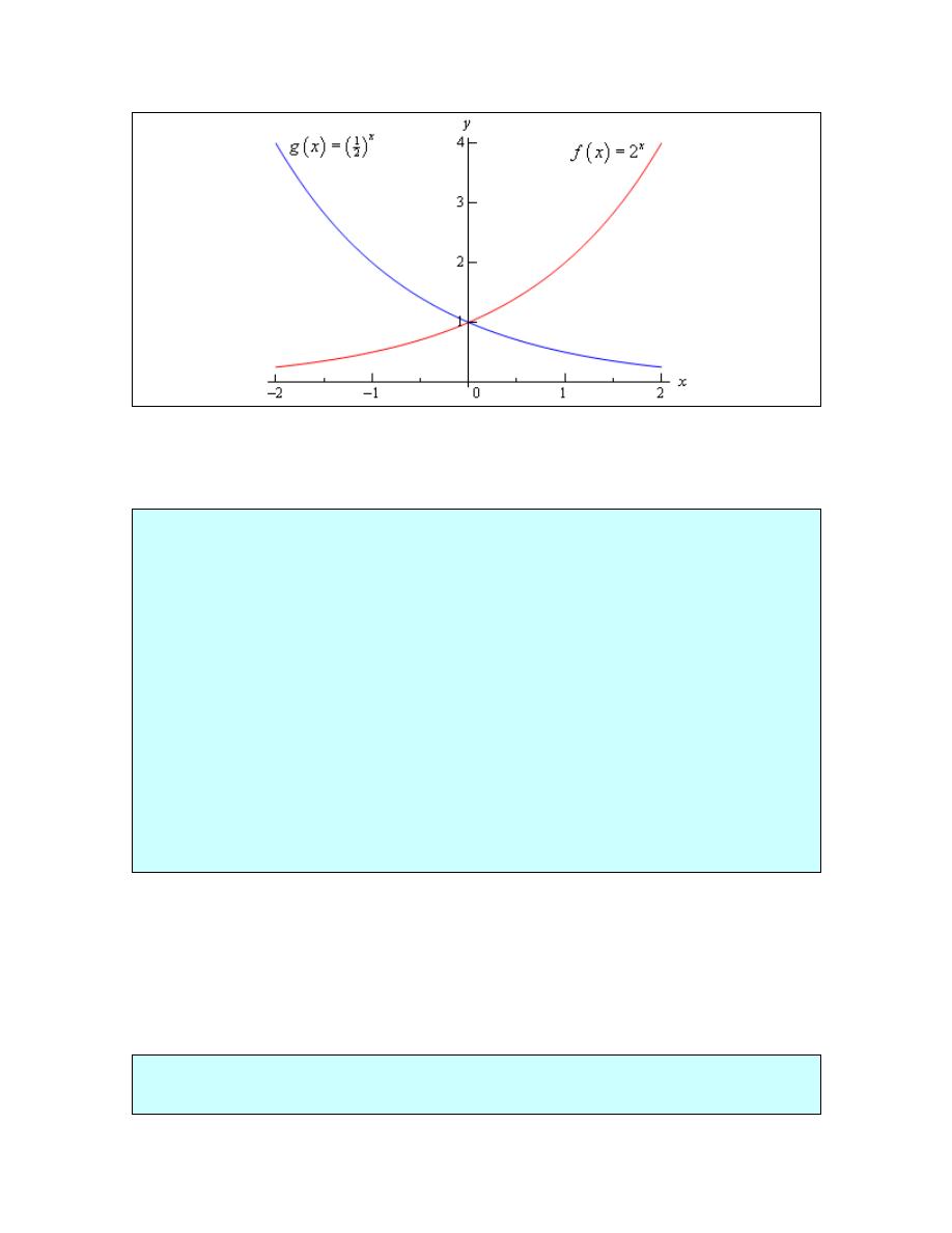
Calculus I

This graph illustrates some very nice properties about exponential functions in general.

Properties of

( )

f x

( )

. The function will always take the value of 1 at

( )

f x

≠

. An exponential function will never be zero.

( )

f x

. An exponential function is always positive.

4. The previous two properties can be summarized by saying that the range of an

exponential function is

(

)

∞

5. The domain of an exponential function is

(

)

−∞ ∞

. In other words, you can plug every x

into an exponential function.

6. If

< <

then,

( )

0 as

f x

→

→ ∞

( )

f x

→ ∞

→ −∞

7. If

then,

( )

f x

→ ∞

( )

0 as

f x

→

→ −∞

These will all be very useful properties to recall at times as we move throughout this course (and
later Calculus courses for that matter…).

There is a very important exponential function that arises naturally in many places. This function
is called the natural exponential function. However, for must people this is simply the
exponential function.

Definition : The natural exponential function is

( )

f x

= e

where,

2.71828182845905



http://tutorial.math.lamar.edu/terms.aspx

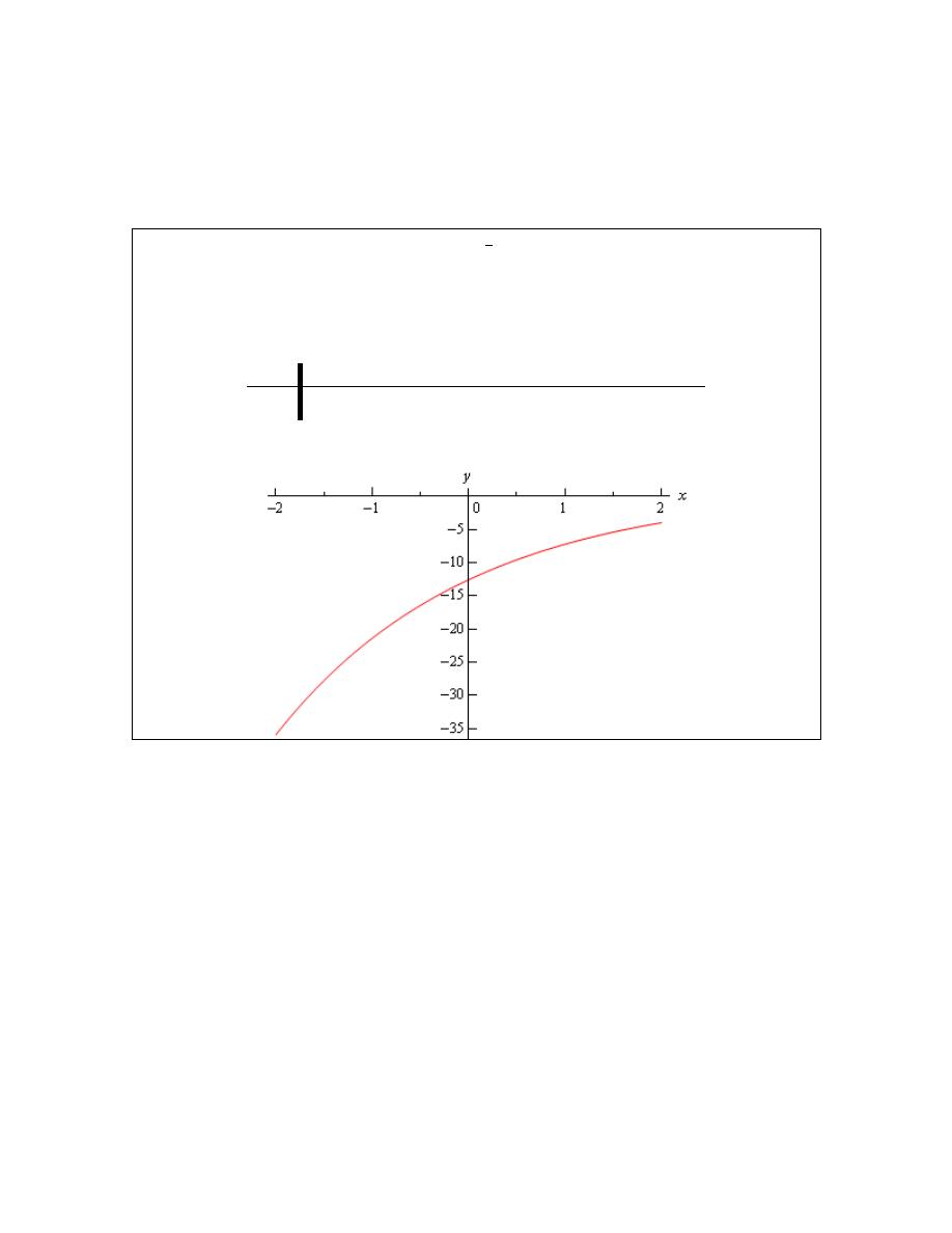
Calculus I

So, since

we also know that

→ ∞

and

0 as

→

→ −∞

Let’s take a quick look at an example.

Example 2 Sketch the graph of

( )

1 5

h t

−

= − e

Solution
Let’s first get a table of values for this function.

-2

-1

( )

h t

-35.9453 -21.4084 -12.5914 -7.2436 -4 -2.0327

Here is the sketch.

The main point behind this problem is to make sure you can do this type of evaluation so make
sure that you can get the values that we graphed in this example. You will be asked to do this
kind of evaluation on occasion in this class.

You will be seeing exponential functions in pretty much every chapter in this class so make sure
that you are comfortable with them.

http://tutorial.math.lamar.edu/terms.aspx

Calculus I

Review : Logarithm Functions

In this section we’ll take a look at a function that is related to the exponential functions we looked
at in the last section. We will look at logarithms in this section. Logarithms are one of the
functions that students fear the most. The main reason for this seems to be that they simply have
never really had to work with them. Once they start working with them, students come to realize
that they aren’t as bad as they first thought.

We’ll start with

≠

just as we did in the last section. Then we have

log

is equivalent to

The first is called logarithmic form and the second is called the exponential form. Remembering
this equivalence is the key to evaluating logarithms. The number, b, is called the base.

Example 1

Without a calculator give the exact value of each of the following logarithms.

(a)

log 16

[

Solution

]

(b)

log 16

[

Solution

]

(c)

log 625

[

Solution

]

(d)

log

531441

[

Solution

]

(e)

log 36

[

Solution

]

(f)

log

[

Solution

]

Solution
To quickly evaluate logarithms the easiest thing to do is to convert the logarithm to exponential
form. So, let’s take a look at the first one.

(a)

log 16

First, let’s convert to exponential form.

log 16

is equivalent to

So, we’re really asking 2 raised to what gives 16. Since 2 raised to 4 is 16 we get,

log 16

because

We’ll not do the remaining parts in quite this detail, but they were all worked in this way.

[

Return to Problems

]

(b)

log 16

because

Note the difference between the first and second logarithm! The base is important! It can
completely change the answer.

[

Return to Problems

]

http://tutorial.math.lamar.edu/terms.aspx

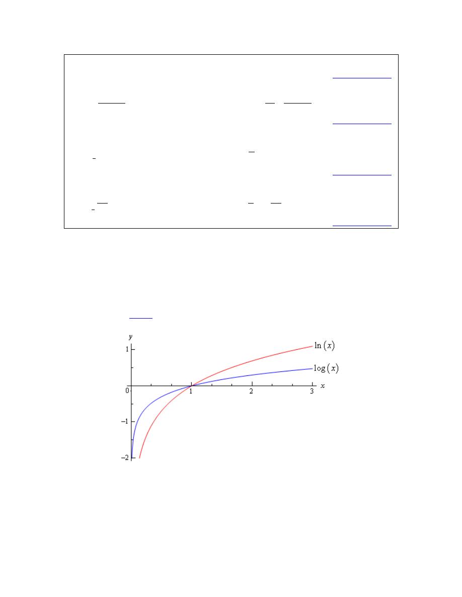
Calculus I

(c)

log 625

because

625

[

Return to Problems

]

(d)

log

because

531441

−

= −

[

Return to Problems

]

(e)

log 36

because

−

 

= −

 

 

[

Return to Problems

]

(f)

log

because

 

 

 

[

Return to Problems

]

There are a couple of special logarithms that arise in many places. These are,

log

This log is called the natural logarithm

log

This log is called the common logarithm

In the natural logarithm the base e is the same number as in the natural exponential logarithm that
we saw in the last

section

. Here is a sketch of both of these logarithms.

From this graph we can get a couple of very nice properties about the natural logarithm that we
will use many times in this and later Calculus courses.

→ ∞

→ −∞

→

http://tutorial.math.lamar.edu/terms.aspx

Calculus I

Let’s take a look at a couple of more logarithm evaluations. Some of which deal with the natural
or common logarithm and some of which don’t.

Example 2

Without a calculator give the exact value of each of the following logarithms.

(a)

ln e

(b)

log1000

(c)

log 16

(d)

log 1

(e)

log

Solution
These work exactly the same as previous example so we won’t put in too many details.

(a)

because

(b)

log1000

because

1000

(c)

log 16 1

because

(d)

log 1

because

(e)

( )

log

because

This last set of examples leads us to some of the basic properties of logarithms.

Properties

1. The domain of the logarithm function is

(

)

∞

. In other words, we can only plug

positive numbers into a logarithm! We can’t plug in zero or a negative number.

log

log 1

log

The last two properties will be especially useful in the next

section

. Notice as well that these last

two properties tell us that,

( )

and

log

f x

g x

are

inverses

of each other.

Here are some more properties that are useful in the manipulation of logarithms.

http://tutorial.math.lamar.edu/terms.aspx

Calculus I

More Properties

log

 

−

 

 

( )

log

Note that there is no equivalent property to the first two for sums and differences. In other words,

(

)

(

)

log

≠

−

≠

−

Example 3

Write each of the following in terms of simpler logarithms.

(a)

ln x y z

[

Solution

]

(b)

log

















[

Solution

]

(c)

(

)

log













−





[

Solution

]

Solution
What the instructions really mean here is to use as many if the properties of logarithms as we can
to simplify things down as much as we can.

(a)

ln x y z

Property 6 above can be extended to products of more than two functions. Once we’ve used
Property 6 we can then use Property 8.

3ln

4 ln

5 ln

x y z

[

Return to Problems

]

(b)

log

















When using property 7 above make sure that the logarithm that you subtract is the one that
contains the denominator as its argument. Also, note that that we’ll be converting the root to
fractional exponents in the first step.

log

log 9

log

log 9 log

log

2 4 log

log





−













−

= +

−

[

Return to Problems

]

http://tutorial.math.lamar.edu/terms.aspx

Calculus I

(c)

(

)

log













−





The point to this problem is mostly the correct use of property 8 above.

(

)

(

)

(

)

(

)

(

)

log

3log





−









−





−

You can use Property 8 on the second term because the WHOLE term was raised to the 3, but in
the first logarithm, only the individual terms were squared and not the term as a whole so the 2’s
must stay where they are!

[

Return to Problems

]

The last topic that we need to look at in this section is the change of base formula for logarithms.
The change of base formula is,

log

This is the most general change of base formula and will convert from base b to base a.
However, the usual reason for using the change of base formula is to compute the value of a
logarithm that is in a base that you can’t easily deal with. Using the change of base formula
means that you can write the logarithm in terms of a logarithm that you can deal with. The two
most common change of base formulas are

log

and

log

In fact, often you will see one or the other listed as THE change of base formula!

In the first part of this section we computed the value of a few logarithms, but we could do these
without the change of base formula because all the arguments could be written in terms of the
base to a power. For instance,

log 49

because

However, this only works because 49 can be written as a power of 7! We would need the change

of base formula to compute

log 50

ln 50

3.91202300543

log 50

2.0103821378

ln 7

1.94591014906

log 50

1.69897000434

log 50

2.0103821378

log 7

0.845098040014

http://tutorial.math.lamar.edu/terms.aspx

Calculus I

So, it doesn’t matter which we use, we will get the same answer regardless of the logarithm that
we use in the change of base formula.

Note as well that we could use the change of base formula on

log 49

if we wanted to as well.

ln 49

3.89182029811

log 49

ln 7

1.94591014906

This is a lot of work however, and is probably not the best way to deal with this.

So, in this section we saw how logarithms work and took a look at some of the properties of
logarithms. We will run into logarithms on occasion so make sure that you can deal with them
when we do run into them.

http://tutorial.math.lamar.edu/terms.aspx

Calculus I

Review : Exponential and Logarithm Equations

In this section we’ll take a look at solving equations with exponential functions or logarithms in
them.

We’ll start with equations that involve exponential functions. The main property that we’ll need
for these equations is,

log

Example 1

Solve

1 3

7 15

−

Solution
The first step is to get the exponential all by itself on one side of the equation with a coefficient of
one.

1 3

7 15

−

=
=

Now, we need to get the z out of the exponent so we can solve for it. To do this we will use the
property above. Since we have an e in the equation we’ll use the natural logarithm. First we take
the logarithm of both sides and then use the property to simplify the equation.

( )

1 3

−

 

=  

 
 

−

=  

 

All we need to do now is solve this equation for z.

1 3

1 ln

0.8698126372

 

−

=  

 

 

− = − +  

 





 

= −

− +

 





 





Example 2

Solve

100

−

Solution
Now, in this case it looks like the best logarithm to use is the common logarithm since left hand
side has a base of 10. There’s no initial simplification to do, so just take the log of both sides and
simplify.

http://tutorial.math.lamar.edu/terms.aspx

Calculus I

log10

log100

−

− =

At this point, we’ve just got a quadratic that can be solved

(

)(

)

− − =

−

+ =

So, it looks like the solutions in this case are

and

= −

Now that we’ve seen a couple of equations where the variable only appears in the exponent we
need to see an example with variables both in the exponent and out of it.

Example 3

Solve

−

Solution
The first step is to factor an x out of both terms.

DO NOT DIVIDE AN x FROM BOTH TERMS!!!!

Note that it is very tempting to “simplify” the equation by dividing an x out of both terms.
However, if you do that you’ll miss a solution as we’ll see.

(

)

−

So, it’s now a little easier to deal with. From this we can see that we get one of two possibilities.

−

The first possibility has nothing more to do, except notice that if we had divided both sides by an
x we would have missed this one so be careful. In the second possibility we’ve got a little more
to do. This is an equation similar to the first two that we did in this section.

ln1

+ =
+ =

= −

Don’t forget that

ln1

So, the two solutions are

and

= −

http://tutorial.math.lamar.edu/terms.aspx

Calculus I

The next equation is a more complicated (looking at least…) example similar to the previous one.

Example 4

Solve

(

) (

)

−

− e

Solution

As with the previous problem do NOT divide an

−

out of both sides. Doing this will lose

solutions even though it “simplifies” the equation. Note however, that if you can divide a term
out then you can also factor it out if the equation is written properly.

So, the first step here is to move everything to one side of the equation and then to factor out the

−

(

) (

)

(

)(

)

4 5

−

− −

−

At this point all we need to do is set each factor equal to zero and solve each.

( )

ln 5

7 ln 5

5.390562088

−

− =

−

= ±

− =

= −

The three solutions are then

= ±

and

5.3906

As a final example let’s take a look at an equation that contains two different logarithms.

Example 5

Solve

1 3

5 2

−

Solution
The first step here is to get one exponential on each side and then we’ll divide both sides by one
of them (which doesn’t matter for the most part) so we’ll have a quotient of two exponentials.
The quotient can then be simplified and we’ll finally get both coefficients on the other side.
Doing all of this gives,

(

)

1 3

5 2

1 3

5 2

1 3

5 2

9
4

−

=
=

http://tutorial.math.lamar.edu/terms.aspx

Calculus I

Note that while we said that it doesn’t really matter which exponential we divide out by doing it
the way we did here we’ll avoid a negative coefficient on the x. Not a major issue, but those
minus signs on coefficients are really easy to lose on occasion.

This is now in a form that we can deal with so here’s the rest of the solution.

( )

(

)

9
4

1
5

4 ln

0.9621860432

−

− =

= +
=

This equation has a single solution of

0.9622

Now let’s take a look at some equations that involve logarithms. The main property that we’ll be
using to solve these kinds of equations is,

log

Example 6

Solve

3 2 ln





= −









Solution
This first step in this problem is to get the logarithm by itself on one side of the equation with a
coefficient of 1.

2 ln





= −













= −









Now, we need to get the x out of the logarithm and the best way to do that is to “exponentiate”
both sides using e. In other word,





−









So using the property above with e, since there is a natural logarithm in the equation, we get,

−

+ = e

Now all that we need to do is solve this for x.

20.78861832

−

+ =

= − +





− +

= −









http://tutorial.math.lamar.edu/terms.aspx

Calculus I

At this point we might be tempted to say that we’re done and move on. However, we do need to
be careful. Recall from the previous

section

that we can’t plug a negative number into a

logarithm. This, by itself, doesn’t mean that our answer won’t work since its negative. What we

need to do is plug it into the logarithm and make sure that

x +

will not be negative. I’ll leave it

to you to verify that this is in fact positive upon plugging our solution into the logarithm and so

20.78861832

= −

is in fact a solution to the equation.

Let’s now take a look at a more complicated equation. Often there will be more than one
logarithm in the equation. When this happens we will need to use on or more of the following
properties to combine all the logarithms into a single logarithm. Once this has been done we can
proceed as we did in the previous example.

( )

log

 

−

 

 

Example 7

Solve

( )

(

)

2 ln

ln 1

−

Solution
First get the two logarithms combined into a single logarithm.

( )

(

)

( )

(

)

( )

(

)

2 ln

ln 1

−



 =





−





Now, exponentiate both sides and solve for x.

(

)

(

)

0.8807970780

−

Finally, we just need to make sure that the solution,

0.8807970780

, doesn’t produce

negative numbers in both of the original logarithms. It doesn’t, so this is in fact our solution to
this problem.

Let’s take a look at one more example.

http://tutorial.math.lamar.edu/terms.aspx

Calculus I

Example 8

Solve

(

)

log

− =

Solution
As with the last example, first combine the logarithms into a single logarithm.

(

)

(

)

(

)

log

x x

− =

−

Now exponentiate, using 10 this time instead of e because we’ve got common logs in the
equation, both sides.

(

)

(

)(

)

log

−

So, potential solutions are

and

= −

. Note, however that if we plug

= −

into either

of the two original logarithms we would get negative numbers so this can’t be a solution. We can

however, use

Therefore, the solution to this equation is

When solving equations with logarithms it is important to check your potential solutions to make
sure that they don’t generate logarithms of negative numbers or zero. It is also important to make
sure that you do the checks in the original equation. If you check them in the second logarithm
above (after we’ve combined the two logs) both solutions will appear to work! This is because in
combining the two logarithms we’ve actually changed the problem. In fact, it is this change that
introduces the extra solution that we couldn’t use!

Also be careful in solving equations containing logarithms to not get locked into the idea that you
will get two potential solutions and only one of these will work. It is possible to have problems
where both are solutions and where neither are solutions.

http://tutorial.math.lamar.edu/terms.aspx

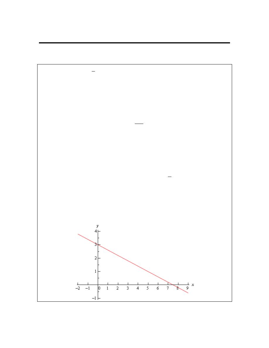
Calculus I

Review : Common Graphs

The purpose of this section is to make sure that you’re familiar with the graphs of many of the
basic functions that you’re liable to run across in a calculus class.

Example 1

Graph

= −

Solution
This is a line in the slope intercept form

mx b

In this case the line has a y intercept of (0,b) and a slope of m. Recall that slope can be thought of
as

rise

run

Note that if the slope is negative we tend to think of the rise as a fall.

The slope allows us to get a second point on the line.  Once we have any point on the line and the
slope we move right by run and up/down by rise depending on the sign. This will be a second
point on the line.

In this case we know (0,3) is a point on the line and the slope is

−

. So starting at (0,3) we’ll

move 5 to the right (i.e.

→

) and down 2 (i.e.

→

) to get (5,1) as a second point on the

line. Once we’ve got two points on a line all we need to do is plot the two points and connect
them with a line.

Here’s the sketch for this line.

http://tutorial.math.lamar.edu/terms.aspx

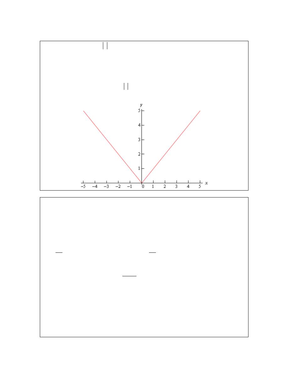
Calculus I

Example 2

Graph

( )

f x

Solution
There really isn’t much to this problem outside of reminding ourselves of what absolute value is.
Recall that the absolute value function is defined as,

if 0

≥



= 

−



The graph is then,

Example 3

Graph

( )

f x

= − +

Solution
This is a parabola in the general form.

( )

f x

bx c

In this form, the x-coordinate of the vertex (the highest or lowest point on the parabola) is

= −

and we get the y-coordinate is





−









. So, for our parabola the coordinates of

the vertex will be.

( )

2 1

= −

−

= −

+ =

So, the vertex for this parabola is (1,4).

We can also determine which direction the parabola opens from the sign of a. If a is positive the
parabola opens up and if a is negative the parabola opens down. In our case the parabola opens
down.

http://tutorial.math.lamar.edu/terms.aspx

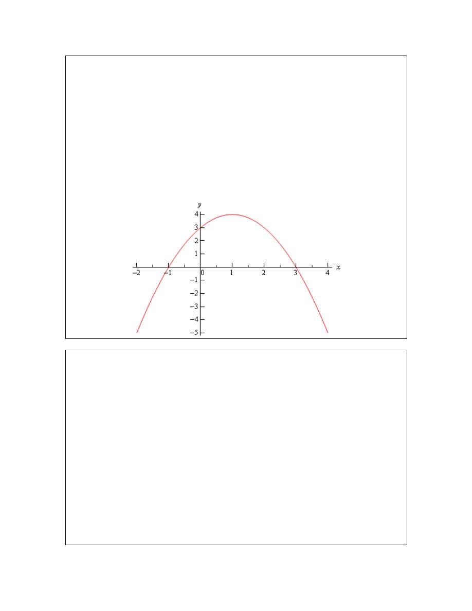
Calculus I

Now, because the vertex is above the x-axis and the parabola opens down we know that we’ll

have x-intercepts (i.e. values of x for which we’ll have

( )

f x

) on this graph. So, we’ll solve

the following.

(

)(

)

− +

+ =

−

− =

−

+ =

So, we will have x-intercepts at

= −

and

. Notice that to make our life easier in the

solution process we multiplied everything by -1 to get the coefficient of the

positive. This

made the factoring easier.

Here’s a sketch of this parabola.

Example 4

Graph

( )

f y

−

Solution
Most people come out of an Algebra class capable of dealing with functions in the form

( )

f x

. However, many functions that you will have to deal with in a Calculus class are in

the form

( )

f y

and can only be easily worked with in that form. So, you need to get used to

working with functions in this form.

The nice thing about these kinds of function is that if you can deal with functions in the form

( )

f x

then you can deal with functions in the form

( )

f y

even if you aren’t that familiar

with them.

Let’s first consider the equation.

−

This is a parabola that opens up and has a vertex of (3,-4), as we know from our work in the
previous example.

http://tutorial.math.lamar.edu/terms.aspx

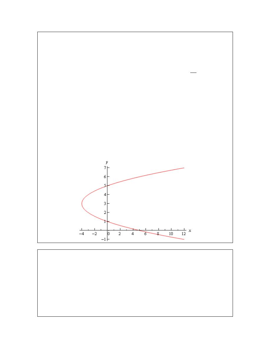
Calculus I

For our function we have essentially the same equation except the x and y’s are switched around.
In other words, we have a parabola in the form,

This is the general form of this kind of parabola and this will be a parabola that opens left or right

depending on the sign of a. The y-coordinate of the vertex is given by

= −

and we find the

x-coordinate by plugging this into the equation. So, you can see that this is very similar to the
type of parabola that you’re already used to dealing with.

Now, let’s get back to the example. Our function is a parabola that opens to the right (a is
positive) and has a vertex at (-4,3). The vertex is to the left of the y-axis and opens to the right so

we’ll need the y-intercepts (i.e. values of y for which we’ll have

( )

f y

)). We find these just

like we found x-intercepts in the previous problem.

(

)(

)

−

+ =

−

− =

So, our parabola will have y-intercepts at

and

. Here’s a sketch of the graph.

Example 5

Graph

−

+ =

Solution
To determine just what kind of graph we’ve got here we need to complete the square on both the
x and the y.

(

) (

)

1 1

16 16 8

−

+ =

+ − +

−

− + =

−

Recall that to complete the square we take the half of the coefficient of the x (or the y), square this

http://tutorial.math.lamar.edu/terms.aspx

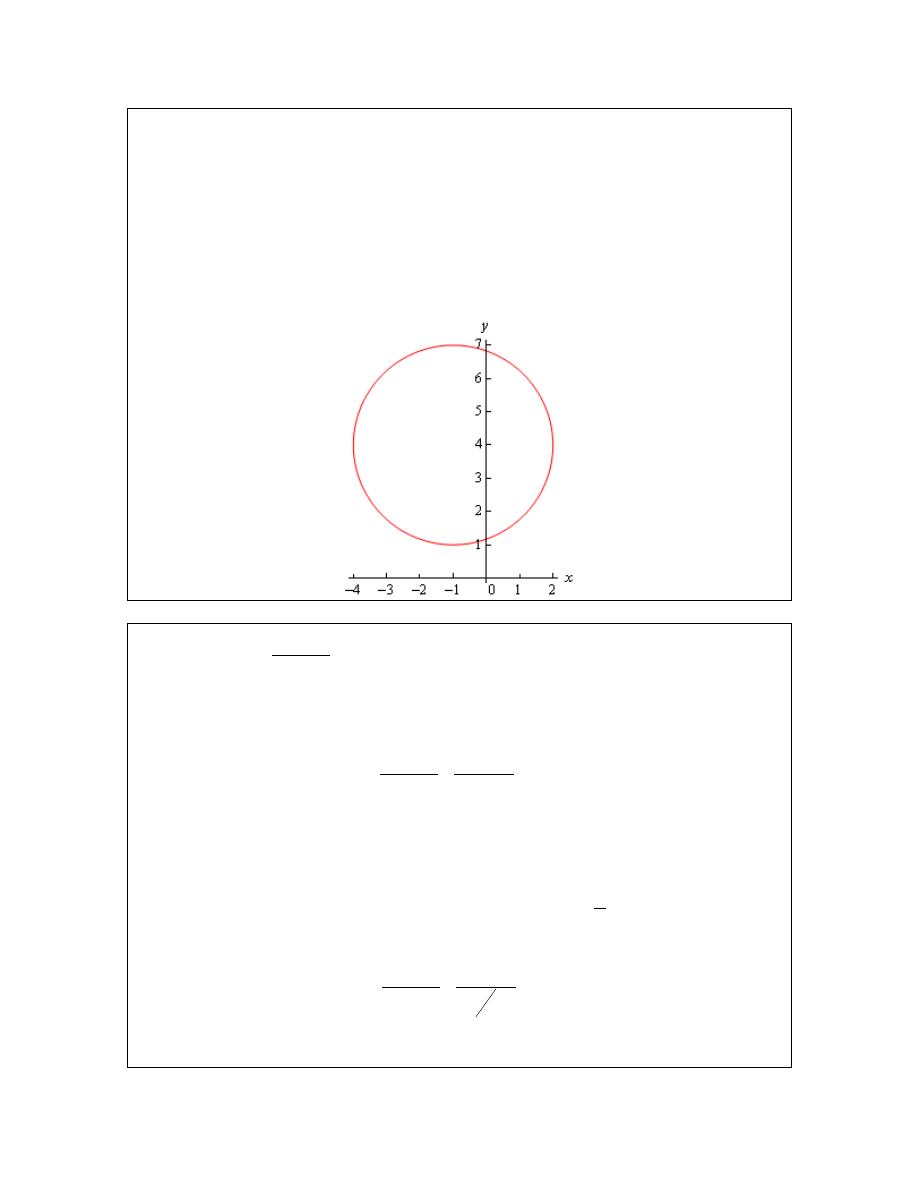
Calculus I

and then add and subtract it to the equation.

Upon doing this we see that we have a circle and it’s now written in standard form.

(

) (

)

−

When circles are in this form we can easily identify the center : (h, k) and radius : r. Once we
have these we can graph the circle simply by starting at the center and moving right, left, up and
down by r to get the rightmost, leftmost, top most and bottom most points respectively.
Our circle has a center at (-1, 4) and a radius of 3. Here’s a sketch of this circle.

Example 6

Graph

(

)

(

)

−

Solution
This is an ellipse. The standard form of the ellipse is

(

) (

)

−

This is an ellipse with center (h, k) and the right most and left most points are a distance of a
away from the center and the top most and bottom most points are a distance of b away from the
center.

The ellipse for this problem has center (2, -2) and has

and

. Note that to get the b

we’re really rewriting the equation as,

(

) (

)

−

to get it into standard from.

http://tutorial.math.lamar.edu/terms.aspx

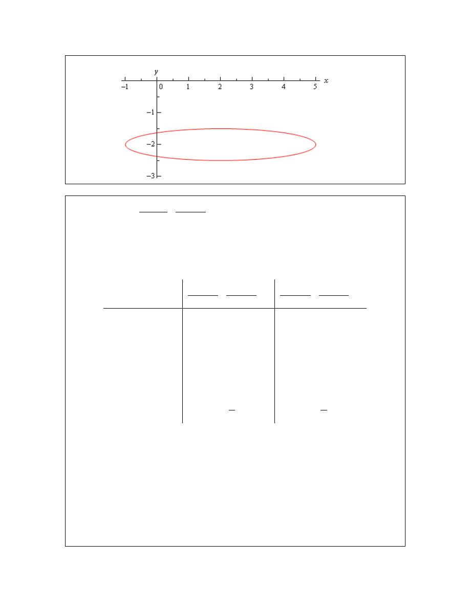
Calculus I

Here’s a sketch of the ellipse.

Example 7

Graph

(

) (

)

−

Solution
This is a hyperbola. There are actually two standard forms for a hyperbola. Here are the basics
for each form.

Form

(

) (

)

−

(

) (

)

x h

−

Center

(h, k)

Opens

Opens right and left

Opens up and down

Vertices

a units right and left
of center.

b units up and down
from center.

Slope of Asymptotes

So, what does all this mean? First, notice that one of the terms is positive and the other is
negative. This will determine which direction the two parts of the hyperbola open. If the x term
is positive the hyperbola opens left and right. Likewise, if the y term is positive the parabola
opens up and down.

Both have the same “center”. Note that hyperbolas don’t really have a center in the sense that
circles and ellipses have centers. The center is the starting point in graphing a hyperbola. It tells
us how to get to the vertices and how to get the asymptotes set up.

The asymptotes of a hyperbola are two lines that intersect at the center and have the slopes listed

http://tutorial.math.lamar.edu/terms.aspx

Calculus I

above. As you move farther out from the center the graph will get closer and closer to the
asymptotes.

For the equation listed here the hyperbola will open left and right. Its center is

(-1, 2). The two vertices are (-4, 2) and (2, 2). The asymptotes will have slopes

Here is a sketch of this hyperbola. Note that the asymptotes are denoted by the two dashed lines.

Example 8

Graph

( )

f x

= e

and

( )

g x

−

= e

Solution
There really isn’t a lot to this problem other than making sure that both of these exponentials are
graphed somewhere.

These will both show up with some regularity in later sections and their behavior as x goes to
both plus and minus infinity will be needed and from this graph we can clearly see this behavior.

http://tutorial.math.lamar.edu/terms.aspx

Calculus I

Example 9

Graph

( )

f x

Solution
This has already been graphed once in this review, but this puts it here with all the other
“important” graphs.

http://tutorial.math.lamar.edu/terms.aspx

Calculus I

Example 10

Graph

Solution
This one is fairly simple, we just need to make sure that we can graph it when need be.

Remember that the domain of the square root function is

≥

Example 11

Graph

Solution
Again, there really isn’t much to this other than to make sure it’s been graphed somewhere so we
can say we’ve done it.

http://tutorial.math.lamar.edu/terms.aspx

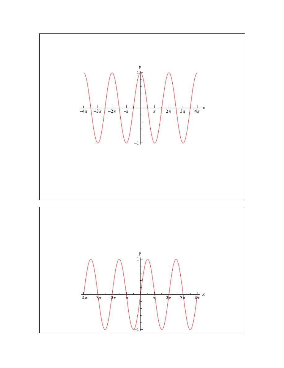
Calculus I

Example 12

Graph

( )

cos

Solution

There really isn’t a whole lot to this one. Here’s the graph for

−

≤ ≤

Let’s also note here that we can put all values of x into cosine (which won’t be the case for most
of the trig functions) and so the domain is all real numbers. Also note that

( )

1 cos

− ≤

≤

It is important to notice that cosine will never be larger than 1 or smaller than -1. This will be
useful on occasion in a calculus class. In general we can say that

( )

cos

− ≤

≤

Example 13

Graph

( )

sin

Solution
As with the first problem in this section there really isn’t a lot to do other than graph it. Here is
the graph.

http://tutorial.math.lamar.edu/terms.aspx

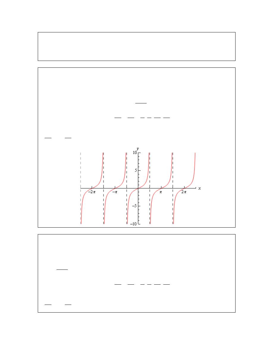
Calculus I

From this graph we can see that sine has the same range that cosine does. In general

( )

sin

− ≤

≤

As with cosine, sine itself will never be larger than 1 and never smaller than -1. Also the domain
of sine is all real numbers.

Example 14

Graph

( )

tan

Solution
In the case of tangent we have to be careful when plugging x’s in since tangent doesn’t exist

wherever cosine is zero (remember that

sin

tan

cos

). Tangent will not exist at

2 2

π π π π

−





and the graph will have asymptotes at these points. Here is the graph of tangent on the range

−

< <

Example 15

Graph

( )

sec

Solution
As with tangent we will have to avoid x’s for which cosine is zero (remember that

sec

cos

). Secant will not exist at

2 2

π π π π

−





and the graph will have asymptotes at these points. Here is the graph of secant on the range

−

< <

http://tutorial.math.lamar.edu/terms.aspx

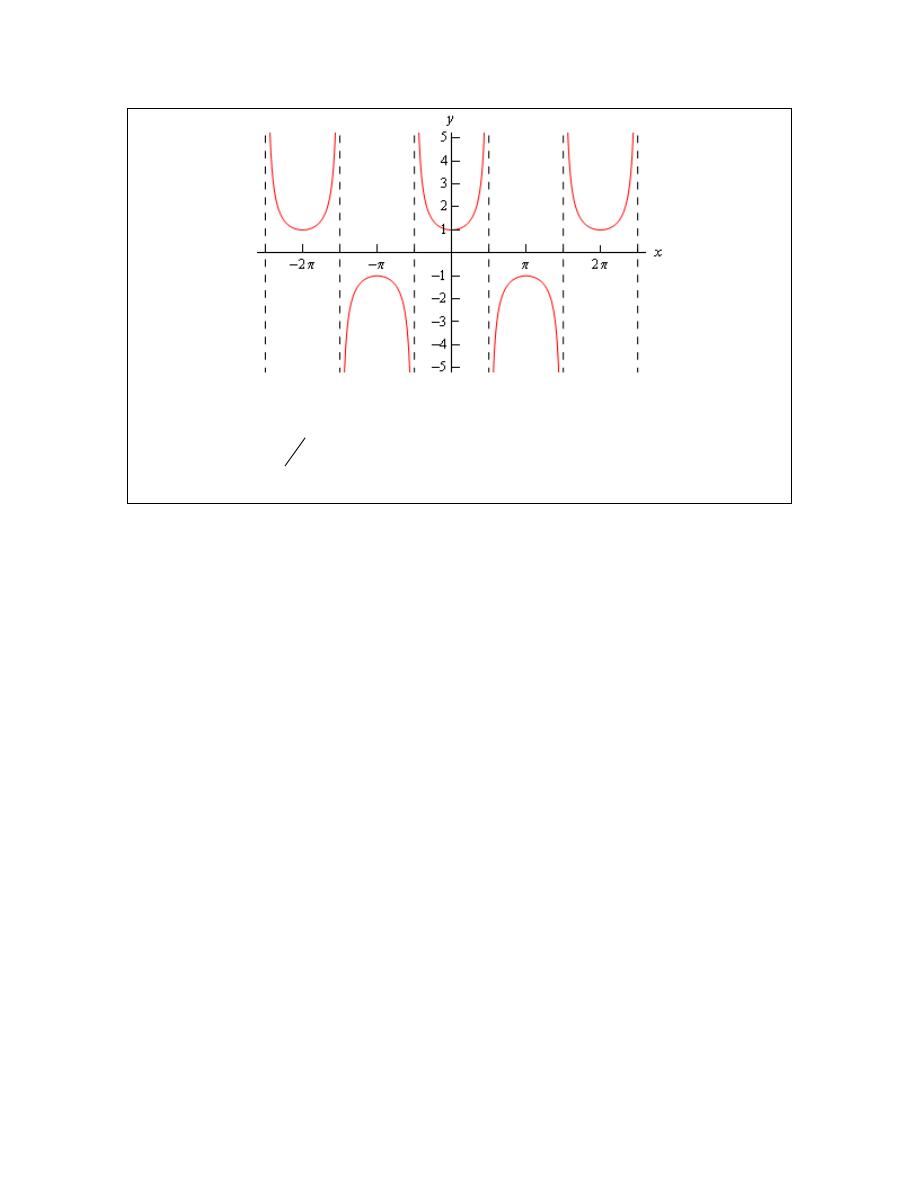
Calculus I

Notice that the graph is always greater than 1 and less than -1. This should not be terribly

surprising. Recall that

( )

1 cos

− ≤

≤

. So, one divided by something less than one will be

greater than 1. Also,

= ±

and so we get the following ranges for secant.

( )

sec

and

sec

≥

≤ −

http://tutorial.math.lamar.edu/terms.aspx

Calculus I

http://tutorial.math.lamar.edu/terms.aspx